HAL Id: hal-01882450
https://hal.archives-ouvertes.fr/hal-01882450
Submitted on 27 Sep 2018
HAL is a multi-disciplinary open access
archive for the deposit and dissemination of
sci-entific research documents, whether they are
pub-lished or not. The documents may come from
teaching and research institutions in France or
abroad, or from public or private research centers.
L’archive ouverte pluridisciplinaire HAL, est
destinée au dépôt et à la diffusion de documents
scientifiques de niveau recherche, publiés ou non,
émanant des établissements d’enseignement et de
recherche français ou étrangers, des laboratoires
publics ou privés.
Alzheimer’s Disease Modelling and Staging through
Independent Gaussian Process Analysis of
Spatio-Temporal Brain Changes
Clement Abi Nader, Nicholas Ayache, Philippe Robert, Marco Lorenzi
To cite this version:
Clement Abi Nader, Nicholas Ayache, Philippe Robert, Marco Lorenzi. Alzheimer’s Disease Modelling
and Staging through Independent Gaussian Process Analysis of Spatio-Temporal Brain Changes.
Ma-chine Learning in Clinical Neuroimaging (MLCN) workshop, Sep 2018, Granada, Spain. �hal-01882450�
through Independent Gaussian Process Analysis
of Spatio-Temporal Brain Changes
Clement Abi Nader1, Nicholas Ayache1, Philippe Robert2,3, and Marco
Lorenzi1, for the Alzheimer’s Disease Neuroimaging Initiative∗
1 UCA, Inria Sophia Antipolis, Epione Research Project 2
UCA, CoBTeK
3 Centre Memoire, CHU de Nice
Abstract. Alzheimer’s disease (AD) is characterized by complex and largely unknown progression dynamics affecting the brain’s morphology. Although the disease evolution spans decades, to date we cannot rely on long-term data to model the pathological progression, since most of the available measures are on a short-term scale. It is therefore difficult to understand and quantify the temporal progression patterns affecting the brain regions across the AD evolution. In this work, we present a generative model based on probabilistic matrix factorization across tem-poral and spatial sources. The proposed method addresses the problem of disease progression modelling by introducing clinically-inspired statis-tical priors. To promote smoothness in time and model plausible patho-logical evolutions, the temporal sources are defined as monotonic and independent Gaussian Processes. We also estimate an individual time-shift parameter for each patient to automatically position him/her along the sources time-axis. To encode the spatial continuity of the brain sub-structures, the spatial sources are modeled as Gaussian random fields. We test our algorithm on grey matter maps extracted from brain struc-tural images. The experiments highlight differential temporal progression patterns mapping brain regions key to the AD pathology, and reveal a disease-specific time scale associated with the decline of volumetric biomarkers across clinical stages.
1
Introduction
Neurodegenerative disorders such as Alzheimer’s disease (AD) are characterized by morphological and molecular changes of the brain, and ultimately lead to *Data used in preparation of this article were obtained from the Alzheimer’s Disease Neuroimaging Initiative (ADNI) database (adni.loni.usc.edu). As such, the investi-gators within the ADNI contributed to the design and implementation of ADNI and/or provided data but did not participate in analysis or writing of this report. A complete listing of ADNI investigators can be found at: http://adni.loni.usc.edu/wp-content/uploads/how to apply/ADNI Acknowledgement List.pdf.
2 C. Abi Nader et al.
cognitive and behavioral decline [8]. To date there is no clear understanding of the dynamics regulating the disease progression. Consequently several attempts have been made to model the disease evolution in a data-driven way, using sets of biomarkers extracted from different imaging acquisition techniques, such as Magnetic Resonance Imaging (MRI) [12]. However available data are mostly represented by cross-sectional measures or time-series acquired on a short-term time span, while the ultimate goal is to unveil the “long-term” disease evolution spreading over decades. Therefore there is a critical need to define the AD evo-lution in a data-driven manner with respect to an absolute time scale associated to the natural history of the pathology.
To this end, in [9] the authors introduce a disease progression score for each patient in order to identify a data-driven disease scale. This score is based on a set of biomarkers and was shown to correlate with the decline of brain cognitive abilities. A similar approach was proposed by [12] and [6] with scalar biomark-ers. In [3], a disease progression score was estimated using higher-dimensional biomarkers from molecular imaging. However these methods don’t provide infor-mation about the brain structures involved in AD, and how the disease affects them along time. To overcome these limitations, [13] proposes a spatio-temporal model of disease progression explicitly accounting for different temporal dynam-ics across the brain. This is done by decomposing cortical thickness measure-ments as a mixture of spatio-temporal processes, by associating each vertex to a temporal progression modeled by a sigmoid function. They also estimate a disease progression score for each subject as a linear transformation of time. However since the proposed formulation does not account for spatial correlation between vertices, it may be potentially sensitive to spatial variation and noise, thus leading to poor interpretability.
The challenge of spatio-temporal modelling in brain images is a classical prob-lem widely addressed via Independent Component Analysis (ICA [7]), especially on functional MRI (fMRI) data [4]. ICA aims at decomposing the data via matrix factorization, looking for a reduced number of spatio-temporal latent sources. Although successful in fMRI analysis, ICA cannot find straightforward applications to the modelling of AD progression. First, ICA retrieves maximally independent latent sources best explaining the data. However, although brain re-gions can exhibit different atrophy rates, this doesn’t necessarily imply statistical independence between them. Second, differently from fMRI data, the absolute time axis of AD spatio-temporal observations is unknown. Thus estimating the pathology timing is a key step in order to model the disease progression, and cannot be performed with standard dimensionality reduction methods such as ICA. Finally, fMRI time series are defined over hundreds of time points, while we work essentially in a cross-sectional setting with one or a few images per-subject. In this work we present a novel spatio-temporal generative model of disease pro-gression aimed at quantifying the independent dynamics of changes in the brain.
We model the observed data through matrix factorization across temporal and spatial sources, with a plausibility constraint introduced by clinically-inspired statistical priors. To promote smoothness in time and model steady evolution from normal to pathological stages, the temporal sources are defined as mono-tonic independent Gaussian Processes (GPs). We also estimate an individual time-shift parameter for each patient to automatically position him along the sources time-axis. To encode the spatial continuity of the brain sub-structures, the spatial sources are modeled as Gaussian random fields. The framework is efficiently optimized through stochastic variational inference. In the next sec-tions we detail the method formulation and show its application on synthetic and real data composed by a large dataset of MRIs from the Alzheimer’s Dis-ease Neuroimaging Initiative (ADNI). Further information can be found in the Appendix*.
2
Method
We assume that the spatio-temporal data Y (x, t) = [Y1(x, t1), Y2(x, t2), .., YP(x, tp)]
is stored in a matrix with dimensions P × F , where P is the number of patients,
F the number of image features, and Yi(x, ti) is the image of an individual i
observed at position x and at time ti. We postulate a generative model in order
to decompose the data in Nsspatio-temporal sources such that :
Yp(x, tp) = S(θ, t + tp)A(ψ, x) + E (1)
Where S is a P ×Nsmatrix where each column represents a temporal trajectory,
tpthe individual time-shift parameter, and θ the set of parameters related to the
temporal sources. A is a Ns× F matrix where each row represents a spatial map,
and ψ is a set of spatial parameters. E is a N (0, σ2I) Gaussian noise. According
to the generative model the likelihood is :
p(Y |A, S, σ) = P Y p=1 1 (2πσ2)F2 exp(− 1 2σ2||Yp− S(θ, t + tp)A(ψ, x)|| 2) (2)
For each row An of A we specify a N (0, I) prior, while each column Sn of S is
a GP modeled as in [5]. This setting leverages on kernel approximation through sampling of basis functions in the spectral domain [14]. For specific choices of the covariance, such as the Radial Basis Function used in our work, the GPs can be approximated as a Bayesian neural network with form : S(t) = φ(Ωt)W . Where Ω is the projection in the spectral domain, φ the non-linear basis function activation, and W the regression parameter. The GPs inference problem thus amounts at estimating approximated distributions for Ω and W .
To account for the steady increase of the sources from normal to pathological stages we introduce a monotonicity prior over the GPs. To do so, we constrain
4 C. Abi Nader et al.
the space of the temporal sources to the set C = {S(t) | S0(t) ≤ 0 ∀t},
follow-ing [11]. This leads to a second likelihood term constrainfollow-ing the dynamics of the temporal sources :
p(C|S0, λ) = (1 + exp(−λS0(t)))−1 (3)
We jointly optimize (2) according to priors and constraints, by maximizing the data evidence : log(p(Y, C|σ, λ)) = log[ Z A Z S Z S0
p(Y |A, S, σ)p(C|S0, λ)p(A)p(S, S0|λ)dAdSdS0]
(4) Since this integral is intractable, we tackle the optimization of (4) via stochastic
variational inference. Following [10] and [5] we introduce approximations q1(A)
and q2(Ω, W ) to derive the lower bound :
log(p(Y, C|σ, λ)) > EA∼q1,(Ω,W )∼q2[log(p(Y |A, Ω, W, σ))] + E(Ω,W )∼q2[log(p(C|Ω, W, λ))]
− D[q1(A)||p(A)] − D[q2(Ω, W )||p(Ω, W )]
(5) Where D refers to the Kullback-Leibler divergence.
We specify the approximated distribution of the spatial activation maps q1such
that q1(A) =Q
N s
n=1N (µn, Σ(α, β)). To introduce spatial correlations in the maps
we choose Σi,j(α, β) = α exp(−||ui− uj||2/2β) to model a smooth decay across
voxels with coordinates (ui, uj). We follow [5] and [11] to also define a
varia-tional lower bound on the constrained GPs parameterizing the temporal pro-cesses. Thanks to the proposed framework, (4) can be efficiently optimized by stochastic variational inference through backpropagation. We chose to alternate the optimization between the spatio-temporal parameters and the time-shift. We set λ to the minimum value that gives monotonic sources, while σ was arbitrarily determined from the data. A detailed derivation of the model and lower-bound can be found in the Appendix.
3
Results
3.1 Benchmark on Synthetic Data
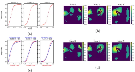
We tested the algorithm on synthetic data to assess its ability to separate spatio-temporal sources from mixed data, and to provide a model selection via the variational lower bound. We generated three monotonically increasing functions
Si(t) such that Si(t) = 1/(1 + exp(−t + αi)), and three synthetic Gausian
acti-vation maps A1, A2, A3 with a 30 × 30 resolution, to mimick grey matter brain
areas (Figures 1a and 1b). The data was generated as Yp,j= S(tp)A + Ej over 40
time points tp, where tp is uniformly distributed in [0,1]. We sampled 50 images
at instants tpand applied our method. To simulate a pure cross-sectional setting
the time associated to each input image was set to zero. Figures 1c and 1d show the estimated spatio-temporal processes when fitting the model with three latent
0.0 0.5 1.0 0.0 0.2 0.4 0.6 0.8 1.0 Source 0 0.0 0.5 1.0 0.0 0.2 0.4 0.6 0.8 1.0 Source 1 0.0 0.5 1.0 0.0 0.2 0.4 0.6 0.8 1.0 Source 2 Time Amplitude (a) Map 0 0.00 0.25 0.50 0.75 1.00 1.25 1.50 1.75 2.00 Map 1 0.00 0.25 0.50 0.75 1.00 1.25 1.50 1.75 2.00 Map 2 0.0 0.5 1.0 1.5 2.0 2.5 (b) 0.0 0.5 1.0 Original Time 0.0 0.2 0.4 0.6 0.8 1.0 0.0 0.5 1.0 Original Time 0.0 0.2 0.4 0.6 0.8 1.0 0.0 0.5 1.0 Original Time 0.0 0.2 0.4 0.6 0.8 1.0 0.250.00 0.25
Estimated Time Estimated Time0.250.00 0.25 Estimated Time0.250.00 0.25
Amplitude (c) Map 0 0.0 0.5 1.0 1.5 2.0 2.5 3.0 Map 1 0.0 0.5 1.0 1.5 2.0 2.5 3.0 Map 2 0.0 0.5 1.0 1.5 2.0 2.5 3.0 (d)
Fig. 1: (a)-(b) Ground truth temporal and spatial sources. (c) Red : raw temporal sources against the original time axis. Blue : recovered temporal sources against the estimated time scale. (d) Estimated spatial maps.
sources. In Figure 2, we see that the individual time-shift parameter estimated for each subject correlates with the original time used to generate the data. This means that the algorithm correctly positions each subject on the temporal trajec-tories.
Fig. 2: The red points represent the val-ues of the estimated subjects’ time-shift against their associated ground truth value.
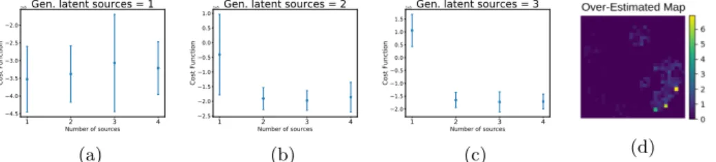
To test the model selection, we gen-erated the data as described above using respectively one, two, or three sources over ten folds. For each fold we ran the algorithm looking for one to four sources. Figure 3 shows mean and standard deviation of the lower bound. We observe that when the number of sources is under-estimated the lower bound is higher. When the number of sources is over-estimated, although the lower bound for model selection is more uncertain, by looking at the extracted spatial maps we ob-serve that the additional sources are mainly set to zero or have low weights (see the map of Figure 3). These ex-perimental results indicate that the optimal number of sources should be
6 C. Abi Nader et al.
selected by inspection of both the lower bound and the extracted spatial sources.
1 2 3 4 Number of sources 4.5 4.0 3.5 3.0 2.5 2.0 Cost Function
1e5Gen. latent sources = 1
(a) 1 2 3 4 Number of sources 2.5 2.0 1.5 1.0 0.5 0.0 0.5 1.0 Cost Function
1e5Gen. latent sources = 2
(b) 1 2 3 4 Number of sources 2.0 1.5 1.0 0.5 0.0 0.5 1.0 1.5 Cost Function
1e5Gen. latent sources = 3
(c) (d)
Fig. 3: (a)-(b)-(c) : Distribution of the lower bound against the number of fitted
sources. (d) : 4thextracted spatial map with data generated by 3 latent sources.
The method was also compared to ICA in a simplified setting by assigning the
ground truth parameter tp beforehand. This simplification is necessary since
standard ICA can’t be applied when the time associated to each image is un-known. We observed that ICA recovered the spatio-temporal sources, by pro-viding however more noisy estimations than the ones we obtained. This result highlights the importance of the priors and constraints introduced in our method (see Appendix).
3.2 Application on Real Data
Data used in the preparation of this article were obtained from the Alzheimer’s Disease Neuroimaging Initiative (ADNI) database (adni.loni.usc.edu). The ADNI was launched in 2003 as a public-private partnership, led by Principal Investiga-tor Michael W. Weiner, MD. For up-to-date information, see www.adni-info.org. In this section we present an application of the algorithm on real data, using grey matter maps extracted from structural MRI. We selected a cohort of 555 subjects from ADNI composed by 94 healthy controls, 343 MCI, and 118 AD pa-tients. We processed the baseline MRI of each subject to obtain high-dimensional grey matter density maps in a standard space [1]. We extracted the 90 × 100 middle coronal slice for each patient, to obtain a data matrix Y with dimen-sions 555 × 9000, and applied our algorithm looking for three spatio-temporal sources (see Figure 4). The middle spatial map shows a strong activation of the hippocampus, while the left and right plots show an activation on the temporal lobes, with two similar temporal behaviours, characterized by a less pronounced grey matter loss compared to the hippocampus. More specifically, we observe that the hippocampal trajectory has a strong acceleration in opposition to the other brain areas. This pattern quantified by our model in a pure data-driven manner is compatible with empirical evidence from clinical studies [2]. In Figure 5 we observe the estimated time of each patient against standard volumetric and
1.0 0.5 0.0 0.5 0.00 0.05 0.10 0.15 0.20 0.25 0.30 Source 0 1.0 0.5 0.0 0.5 0.00 0.05 0.10 0.15 0.20 0.25 0.30 0.35 0.40 Source 1 1.0 0.5 0.0 0.5 0.00 0.05 0.10 0.15 0.20 0.25 0.30 Source 2 Estimated Time Amplitude (a)
Map 0
0.5 1.0 1.5 2.0Map 1
0.5 1.0 1.5 2.0 2.5Map 2
0.25 0.50 0.75 1.00 1.25 1.50 1.75 (b)Fig. 4: (a)-(b) Temporal and Spatial sources extracted from the data.
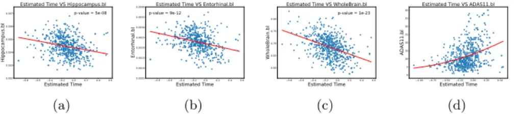
clinical biomarkers. We see a strong correlation between brain volumetric mea-sures and the estimated time, as well as a non-linear relation in the evolution of ADAS11. The latter result indicates an acceleration of clinical symptoms along the estimated time course.
0.8 0.6 0.4 0.2 0.0 0.2 0.4 0.6 Estimated Time 0.002 0.003 0.004 0.005 0.006 0.007 Hippocampus.bl
Estimated Time VS Hippocampus.bl
p-value = 5e-08 (a) 0.8 0.6 0.4 0.2 0.0 0.2 0.4 0.6 Estimated Time 0.0005 0.0010 0.0015 0.0020 0.0025 0.0030 0.0035 0.0040 Entorhinal.bl
Estimated Time VS Entorhinal.bl
p-value = 9e-12 (b) 0.8 0.6 0.4 0.2 0.0 0.2 0.4 0.6 Estimated Time 0.60 0.65 0.70 0.75 0.80 WholeBrain.bl
Estimated Time VS WholeBrain.bl
p-value = 1e-23 (c) 1.00 0.75 0.50 0.25 0.00 0.25 0.50 Estimated Time 0 5 10 15 20 25 30 35 40 ADAS11.bl
Estimated Time VS ADAS11.bl
(d)
Fig. 5: Evolution of volumetric and clinical biomarkers along the estimated time.
4
Conclusion
We presented a method for analyzing spatio-temporal data, which provides both independent spatio-temporal processes at stake in AD, and a disease progression scale. Applied on grey matter maps, the model highlights different brain regions affected by the disease, such as the hippocampus and the temporal lobes, along with their differential temporal trajectory. We also show a strong correlation between the estimated disease progression scale and different clinical and vol-umetric biomarkers. We are currently extending the approach to scale to 3D volumetric images by parallelization on multiple GPUs. The lower bound prop-erties will be also further investigated to better assess its reliability, in order to improve the model comparison. Moreover the method will be extended beyond the cross-sectional application of 3.2, to account for time-series of brain images, as well as for multimodal imaging biomarkers. Finally we will investigate the use of the approach for prognosis purposes, to provide a data-driven assessment of disease severity in testing patients.
8 C. Abi Nader et al.
5
Acknowledgements
This work has been supported by the French government, through the UCAJEDI
Investments in the Future project managed by the National Research Agency
(ref.n ANR-15-IDEX-01), the grant AAP Sant´e 06 2017-260 DGA-DSH, and by
the Inria Sophia Antipolis - M´editerran´ee, ”NEF” computation cluster.
References
1. Ashburner, J.: A fast diffeomorphic image registration algorithm. NeuroImage 38(1), 95 – 113 (2007)
2. Bateman, R.J., et al.: Clinical and biomarker changes in dominantly inherited alzheimer’s disease. New England Journal of Medicine 367(9), 795–804 (2012), pMID: 22784036
3. Bilgel, M., et al.: Temporal Trajectory and Progression Score Estimation from Voxelwise Longitudinal Imaging Measures: Application to Amyloid Imaging. Inf Process Med Imaging 24, 424–436 (2015)
4. Calhoun, V.D., et al.: A review of group ICA for fMRI data and ICA for joint inference of imaging, genetic, and ERP data. Neuroimage 45(1 Suppl), S163–172 (Mar 2009)
5. Cutajar, K., et al.: Random feature expansions for deep Gaussian processes. In: Precup, D., Teh, Y.W. (eds.) Proceedings of the 34th International Conference on Machine Learning. Proceedings of Machine Learning Research, vol. 70, pp. 884– 893. PMLR, International Convention Centre, Sydney, Australia (06–11 Aug 2017) 6. Donohue, M.C., et al.: Estimating long-term multivariate progression from
short-term data. Alzheimer’s & Dementia 10(5, Supplement), S400 – S410 (2014) 7. Hyv¨arinen, A., Oja, E.: Independent component analysis: algorithms and
applica-tions. Neural Networks 13, 411–430 (2000)
8. Jack, C.R., et al.: Hypothetical model of dynamic biomarkers of the Alzheimer’s pathological cascade. Lancet Neurol 9(1), 119–128 (Jan 2010)
9. Jedynak, B.M., et al.: A computational neurodegenerative disease progression score: method and results with the Alzheimer’s disease Neuroimaging Initiative cohort. Neuroimage 63(3), 1478–1486 (Nov 2012)
10. Kingma, D.P., Welling, M.: Auto-encoding variational bayes. CoRR abs/1312.6114 (2013)
11. Lorenzi, M., Filippone, M.: Constraining the dynamics of deep probabilistic models. In: Dy, J., Krause, A. (eds.) Proceedings of the 35th International Conference on Machine Learning. Proceedings of Machine Learning Research, vol. 80, pp. 3233– 3242. PMLR, Stockholmsm¨assan, Stockholm Sweden (10–15 Jul 2018)
12. Lorenzi, M., et al.: Probabilistic disease progression modeling to characterize di-agnostic uncertainty: Application to staging and prediction in alzheimer’s disease. NeuroImage (2017)
13. Marinescu, R.V., et al.: A vertex clustering model for disease progression: Appli-cation to cortical thickness images. In: Niethammer, M., et al. (eds.) Information Processing in Medical Imaging. pp. 134–145. Springer International Publishing, Cham (2017)
14. Rahimi, A., Recht, B.: Random features for large-scale kernel machines. In: Platt, J.C., et al. (eds.) Advances in Neural Information Processing Systems 20, pp. 1177–1184. Curran Associates, Inc. (2008)