HAL Id: hal-00292334
https://hal.archives-ouvertes.fr/hal-00292334
Submitted on 1 Jul 2008
HAL is a multi-disciplinary open access
archive for the deposit and dissemination of sci-entific research documents, whether they are pub-lished or not. The documents may come from teaching and research institutions in France or abroad, or from public or private research centers.
L’archive ouverte pluridisciplinaire HAL, est destinée au dépôt et à la diffusion de documents scientifiques de niveau recherche, publiés ou non, émanant des établissements d’enseignement et de recherche français ou étrangers, des laboratoires publics ou privés.
A family of generalized gamma convoluted variables
Bernard Roynette, Pierre Vallois, Marc Yor
To cite this version:
Bernard Roynette, Pierre Vallois, Marc Yor. A family of generalized gamma convoluted variables. Probability and Mathematical Statistics, 2009, 29 (2), pp.181-204. �hal-00292334�
A family of generalized gamma convoluted variables
B. Roynette(1), P. Vallois(1)M. Yor(2), (3)
26/05/2008
(1) Institut Elie Cartan, Universit´e Henri Poincar´e,
B.P. 239, 54506 Vandoeuvre les Nancy Cedex
(2) Laboratoire de Probabilit´es et Mod`eles Al´eatoires,
Universit´e Paris VI et VII, 4 place Jussieu - Case 188 F - 75252 Paris Cedex 05
(3) Institut Universitaire de France
Abstract This paper consists of three parts : in the first part, we describe a family of generalized gamma convoluted (abbreviated as GGC) variables. In the second part, we use this description to prove that several r.v.’s, related to the length of excursions away from 0 for a recurrent linear diffusion on R+, are GGC. Finally, in the third part, we apply our results
to the case of Bessel processes with dimension d = 2(1− α) (0 < d < 2, or 0 < α < 1). Key words : 60 J 25, 60 G 51, 60 E 07, 60 E 05.
0
Notation and Introduction
0.1 Let l : R+→ R+ denote a Borel function such that :
Z ∞
0
l(z)
z dz <∞ (0.1)
Without loss of generality, we assume that : Z ∞
0
l(z)
z dz = 1 (0.2)
With l, we associate a r.v. Y on R+ whose probability density fY is given by :
fY(u) =
Z ∞
0
e−uzl(z)dz (u≥ 0) (0.3)
Indeed, due to (0.2), we get : Z ∞ 0 fY(u)du = Z ∞ 0 du Z ∞ 0 e−uzl(z)dz = Z ∞ 0 l(z) z dz = 1 (0.4)
To emphasize the relation between Y and l, we shall (sometimes) write Yl.
We denote by ϕl≡ ϕYl the Laplace transform of Yl :
ϕl(λ) = ϕYl(λ) = E(e−λYl) = Z ∞ 0 e−λufYl(u)du = Z ∞ 0 l(z) λ + z dz (0.5)
0.2 A reminder about GGC variables
Let µ denote a positive, σ-finite measure on R+. We recall¡see [Bon]¢ that a positive r.v. Y
is a GGC variable with Thorin measure µ if : E(e−λY) = exp
½ − Z ∞ 0 (1− e−λx)dx x Z ∞ 0 e−xzµ(dz) ¾ (λ≥ 0) (0.6)
Such a r.v. is self-decomposable, hence infinitely divisible.
The GGC r.v.’s Y whose Thorin measure µ has a finite total mass, equal to m, are charac-terized by¡see [JRY]¢ :
E(e−λY) = exp ½ −m Z ∞ 0 (1− e−λx)dx x E(e −xG) ¾ (0.7) where G is an R+-valued r.v. such that E¡ log+(1/G)¢ < ∞.
Such a r.v. is a gamma-m mixture, i.e. it satisfies1 :
Y (law)= γm· Z (0.8)
where γm is a gamma variable with parameter m, independent from the R+-valued variable
Z. We note that any r.v. which is a gamma-m mixture is also a gamma-m′ mixture, for any m′ > m, since there is the identity :
γm (law)
= γm′· βm, m′−m (0.9)
where γm′ is a gamma variable with parameter m′ and βm, m′−m is a beta variable with
parameters (m, m′− m) independent from γm′.
We also recall¡see [Bon], p. 51¢ that the parameter m of a GGC r.v. Y , with Thorin measure with total mass m, may be obtained from the formula :
m = sup ½ δ ≥ 0 ; lim u↓0+ fY(u) uδ−1 = 0 ¾ (0.10)
1
A family of GGC variables
The aim of this part is to present a sufficient condition on l which implies that the associated variable Yl is GGC.
Definition 1 A function l which satisfies (0.1) belongs to the class C if there exist a ≥ 0, b > a, σ≥ 0 and θ : R+ → R ∪ (+∞) a Borel, decreasing function, which is identically equal
to +∞ on [0, a[, such that : l(z) = exp ½ σ + Z z b θ(y) y dy ¾ (1.1)
1It would be more correct to say that : the law of such a r.v. is a gamma-m mixture ; however, such abuse
Of course, if (1.1) is satisfied with a > 0, then the function l is identically 0 on [0, a[.
On the other hand, if l is identically 0 on [0, a[ and differentiable on ]a,∞[, then l belongs to the classC if and only if the function :
y → y (log l)′(y) := θ(y) (1.2)
is decreasing on [a,∞[.
The following properties are elementary :
• If l ∈ C, then for every u > 0, x → l(ux) ∈ C (1.3)
• If l1, l2 ∈ C, then l1· l2 ∈ C (1.4)
• For every α real, x → xα∈ C (1.5)
• For every k < 0 and γ ≥ 0, x → (x + γ)k∈ C (1.6) Theorem 2 Let l which satisfies (0.2) and belongs toC, and let Yl denote the r.v. associated
with l. Then :
Yl is a GGC r.v. whose Thorin measure µ has total mass m smaller than or equal to 1. In
other terms, there exists a r.v. G taking values in R+, and satisfying E¡ log+(1/G)¢ < ∞
and m≤ 1 such that : E(e−λYl) = exp
½ −m Z ∞ 0 (1− e−λx)dx x E(e −xG) ¾ (λ≥ 0) (1.7) Proof of Theorem 2
1. It suffices to show that Ylis GGC since, if so, then the total mass m of its Thorin measure
equals, from (0.3) and (0.10) : m = sup ½ δ ≥ 0 ; lim u↓0+ 1 uδ−1 Z ∞ 0 e−uzl(z)dz = 0 ¾
and, of course, m≤ 1 since, for δ = 1 : 1 uδ−1 Z ∞ 0 e−uzl(z)dz = Z ∞ 0 e−uzl(z)dz−→ u↓0+ Z ∞ 0 l(z)dz > 0
2. To show that Yl is GGC, we shall use the following characterization¡see [Bon], Th. 6.1.1,
p. 90¢ of these r.v.’s :
Y is GGC if and only if its Laplace transform ϕY is hyperbolically completely monotone, that
is it satisfies : for every u > 0, the function Hu, defined by :
Hu(w) = ϕY(uv)· ϕY ³u v ´ , where w = v + 1 v (1.8)
is a completely monotone function, i.e. it is the Laplace transform of a positive measure carried by R+.
In our framework, this criterion becomes : for every u > 0, Hu is completely monotone with,
from (0.5) : Hu(w) = Z ∞ 0 Z ∞ 0 l(x)l(y) (x + uv)(y + uv) dx dy µ w = v + 1 v ¶ (1.9) = Z ∞ 0 Z ∞ 0 l(ux)l(uy) (x + v)(y + 1v) dx dy (1.10)
(after the change of variables x = ux′, y = uy′).
Our aim being to show that the hypothesis : l∈ C implies that Hu is completely monotone,
and since x→ l(ux) belongs to C if l ∈ C ¡from (1.3)¢, it suffices to see that the function H defined by : H(w) := Z ∞ 0 Z ∞ 0 l(x)l(y) (x + v)(y + 1v) dx dy µ w = v + 1 v ¶ (1.11) is completely monotone.
3. We show that H, defined by (1.11), is completely monotone : i) We write : H(w) = Z ∞ 0 Z ∞ 0 l(x)l(y) (x + v)(y +1v) dx dy = 1 2 Z ∞ 0 Z ∞ 0 l(x)l(y) " 1 (x + v)(y + 1v) + 1 (x + 1v)(y + v) # dx dy (by symmetry) = 1 2 Z ∞ 0 Z ∞ 0 l(x)l(y)· x 2− 1 xy− 1· 1 x2+ xw + 1 + y2− 1 xy− 1· 1 y2+ yw + 1 ¸ dx dy (1.12)
(after reducing both reciprocals to the same denominator and decomposing into simple ele-ments) = 1 2 Z ∞ 0 Z ∞ 0 l(x)l(y)dx dy · x 2− 1 xy− 1 Z ∞ 0 e−b(x2+xw+1)db + y 2− 1 xy− 1 Z ∞ 0 e−b(y2+yw+1)db ¸ = 1 2 Z ∞ 0 Z ∞ 0 l(x)l(y)dx dy·· x 2− 1 xy− 1· 1 x Z ∞ 0 e−bw−b(x+1x)db + y 2− 1 xy− 1 1 ye −bw−b(y+1 y)db ¸
(after making the change of variables bx = b′, by = b′) = Z ∞ 0 e−bwdb µZ ∞ 0 Z ∞ 0 l(x)l(y) x 2− 1 (xy− 1)x e −b(x+1 x)dx dy ¶ (1.13) after interverting the orders of integration.
We note that the preceding computation is a little formal : we have transformed an absolutely convergent integral in an integral which is no longer absolutely convergent ; however, this does not matter for our purpose, as we shall soon gather the different terms in another way.
ii) Thus, we need to show, from (1.13), that, for every b≥ 0 : Ib:= Z ∞ 0 Z ∞ 0 l(x)l(y) x 2− 1 (xy− 1)xe−b(x+ 1 x)dx dy≥ 0 (1.14)
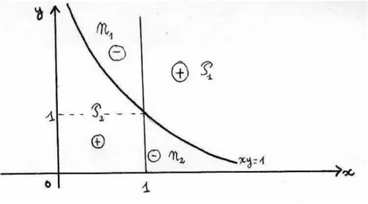
• Let us show (1.14). For this purpose, we define the 4 domains : N1= ½ 0 < x≤ 1, y > 1 x ¾ , N2 = ½ x≥ 1, y < 1 x ¾ P1= ½ x≥ 1, y > 1 x ¾ , P2 = ½ 0 < x≤ 1, y < 1 x ¾
Figure 1 Let us define : ψ(x, y) := l(x)l(y) x 2− 1 (xy− 1)x e−b(x+ 1 x) (1.15)
It is clear that ψ is negative onN1 and N2 and positive on P1 andP2. We note :
Ni:= Z Z Ni |ψ(x, y)|dx dy (i = 1, 2) Pi := Z Z Pi ψ(x, y) dx dy (i = 1, 2)
• To prove (1.14) it suffices to see that : Ni ≤ Pi (i = 1, 2). To compute N1 and P2 ¡ ⊂
{(x, y) ∈ R2+; x≤ 1}¢, we make the change of variables for x ∈]0, 1], t ≥ 2 : x =
t−√t2− 4 2 ; so : 1 x = t +√t2− 4 2 , x + 1 x = t, x2− 1 x2 dx = dt. We obtain : N1 = Z ∞ 2 dt Z ∞ t+√t2−4 2 dy l à t−√t2− 4 2 ! l(y) e−bt y−t+√2t2−4 = Z ∞ 2 dt Z ∞ 0 dz l à t−√t2− 4 2 ! l Ãà t +√t2− 4 2 ! (1 + z) ! e−bt z (1.16)
³
after making the change of variable y = (1 + z)³t+√2t2−4´´
P2 = Z ∞ 2 dt Z 1 0 dz l à t−√t2− 4 2 ! l Ãà t +√t2− 4 2 ! (1− z) ! e−bt z (1.17)
To compute N2 and P1 ¡ ⊂ {(x, y) ∈ R2+; x≥ 1}¢ for x ≥ 1, t ≥ 2 we make the change of
variable : x = t + √ t2− 4 2 . So 1 x = t−√t2− 4 2 , x + 1 x = t and x2− 1 x2 dx = dt. We obtain : N2= Z ∞ 2 dt Z 1 0 dz l à t +√t2− 4 2 ! l Ãà t−√t2− 4 2 ! (1− z) ! e−bt z (1.18) P1 = Z ∞ 2 dt Z ∞ 0 dz l à t +√t2− 4 2 ! l Ãà t−√t2− 4 2 ! (1 + z) ! e−bt z (1.19)
We shall now use the hypothesis : l belongs toC to show that : P1 ≥ N1 and P2 ≥ N2
which will end the proof of our Theorem.
• Comparing (1.19) and (1.16), it suffices, to prove that P1 ≥ N1 to show that :
l à t +√t2− 4 2 ! l Ãà t−√t2− 4 2 ! (1 + z) ! ≥ l à t−√t2− 4 2 ! l Ãà t +√t2− 4 2 ! (1 + z) ! i.e. : lµ 1 x ¶ l(c x)≥ l(x) · l³c x ´ (1.20) with x≤ 1 and c ≥ 1.
If a≥ 1 (a being featured in the definition of C), the relation (1.20) is trivially satisfied since l(x) = 0 for x≤ a (and x ≤ 1).
We now examine the case 0≤ a < 1.
If x≤ a, the relation (1.20) is again trivially satisfied. Thus, let us assume that 1 ≥ x ≥ a. Relation (1.20) is equivalent to
log lµ 1 x
− log l(x) ≥ log l³xc´− log (c x) or also to : Z 1/x x θ(y) y dy− Z c/x cx θ(y) y dy≥ 0 (1.21) ¡since log l(x) = σ + Z x b θ(y) y dy, from (1.1)¢. Thus, (1.21) is equivalent to : Z 1/x x θ(y) y dy− c Z 1/x x θ(cy) cy dy = Z 1/x x θ(y)− θ(cy) y dy≥ 0 (1.22)
and (1.22) is satisfied since θ is decreasing (and c≥ 1). We have shown that P1 ≥ N1.
We now show that P2 ≥ N2 :
This time, using (1.17) and (1.18) it suffices to show that : l à t−√t2− 4 2 ! l à t +√t2− 4 2 (1− z) ! ≥ l à t +√t2− 4 2 ! l à t−√t2− 4 2 (1− z) ! or, equivalently : l(x) l³c x ´ ≥ lµ 1 x ¶ l(cx) with x≤ 1 and c ≤ 1 (1.23)
Relation (1.23) is trivial for x≤ a¡since cx ≤ a and l(cx) = 0¢. It remains to examine the case x≥ a, a ≤ 1. Relation (1.23) is then equivalent to :
Z c x cx θ(y) y dy− Z 1 x x θ(y) y dy≥ 0, i.e. Z 1 x x θ(cy)− θ(y) y dy≥ 0.
The latter relation is obvious since θ is decreasing (and c < 1). This ends the proof of
Theorem 2. ¥
Remark 3 Recall (see (1.8) above) that a function ϕ : R+→ R+is said to be hyperbolically
completely monotone (HCM) if, for every u > 0, the function of w : v + 1 v = w−→ ϕ(uv)ϕ ³u v ´ (with v≥ 0)
is completely monotone. Thus, from (0.5), our Theorem 2 may be stated as follows : if l belongs toC then its Stieltjes transform is HCM.
2
Application to some r.v.’s related to recurrent linear
diffu-sions
2.1 Our notation and hypotheses are now those of Salminen-Vallois-Yor ¡[SVY]¢ to which we refer the reader. (Xt, t≥ 0) denotes a R+-valued diffusion which is recurrent ; we denote
its speed measure (assumed to have no atoms) by m and its scale function by S. (Lt, t≥ 0)
denotes the (continuous) local time at 0 and (τu, u≥ 0) its right-continuous inverse :
τu:= inf{t ≥ 0 ; Lt> u} (2.1)
(τu, u ≥ 0) is a subordinator whose L´evy measure admits a density ¡see [SVY]¢ which we
shall denote by ν : E(exp−λτu) = exp ½ −u Z ∞ 0 (1− e−λx)ν(x)dx ¾ (2.2) In fact, ν may be expressed in the form :
ν(x) = Z ∞
0
e−xzK(dz) (2.3)
where K - the Krein measure -¡see Kotani-Watanabe [K.W], Knight [K]¢ satisfies : Z ∞ 0 K(dz) z(1 + z) <∞ and Z ∞ 0 K(dz) z =∞ (2.4)
2.2 Let, for every t≥ 0 :
gt:= sup{s ≤ t ; Xs= 0}, dt:= inf{s ≥ t ; Xs = 0} (2.5)
and denote by ep (p > 0) an exponentially distributed variable with parameter p, i.e. with
density fep(u) = p e−pu1u≥0 ; ep is assumed to be independent from (Xt, t≥ 0). We define :
Yp(1):= ep− gep, Yp(2) := dep− ep Yp(3):= dep− gep (2.6)
It is shown in [SVY], Theorem 16, that for i = 1, 2, 3, Yp(i) is infinitely divisible.
More precisely, concerning Yp(3), it is shown that Yp(3) is a gamma-2 mixture, which implies
from Kristiansen¡see [Kr]¢ that Yp(3) is infinitely divisible.
The aim of the following Theorem 4 is to improve, if possible, the results we just recalled. More precisely, we shall prove that, under certain hypotheses the r.v.’s Yp(2) (i = 1, 2, 3) are
GGC r.v.’s whose Thorin measures have total masses m≤ 1. Thus, these variables : - are GGC, hence are self-decomposable, and a fortiori are infinitely divisible, - are gamma-m mixtures, with m≤ 1, and not only gamma-2 mixtures¡see (0.9)¢.
Theorem 4 We assume that Krein’s measure K ¡defined by (2.3)¢ admits a differentiable density k. 1. Assume that : k′ k(x) = 1 x + θ(p + x) p + x , with θ decreasing, (2.7)
then Yp(1) is a GGC r.v. whose Thorin measure is a subprobability.
2. Assume that : k′ k(x) = 1 x + p+ θ(x) x , with θ decreasing (2.8)
then Yp(2) is a GGC r.v. whose Thorin measure is a subprobability.
3. Assume that : k′ k(z) = θ(z) z for z < p k′(z)− k′(z− p) k(z)− k(z − p) = θ(z) z for z≥ p (2.9) with θ decreasing
Proof of Theorem 4 We denote by f
Yp(i) the density of Y
(i)
p . From [SVY], p. 115, we have :
f Yp(1)(u) = C1(p) Z ∞ p e−uz·k(z− p) z− p dz (2.10) f Yp(2)(u) = C2(p) Z ∞ 0 e−uz k(z) z + p dz (2.11) f Yp(3)(u) = C3(p) Z ∞ 0 e−uz¡k(z) − 1{z≥p}k(z− p)¢dz (2.12)
where Ci(p), i = 1, 2, 3 are three normalising constants. We shall now use Theorem 2 with,
successively : l(1)(x) = C1(p) k(x− p) x− p 1x≥p (2.13) l(2)(x) = C2(p) k(x) x + p (2.14) l(3)(x) = C3(p)¡k(x) − 1x≥pk(x− p)¢ (2.15)
We already note that, for i = 1, 2, 3, Z ∞ 0 l(i)(x) x dx <∞. Indeed : Z ∞ 0 l(1)(x) x dx = C1(p) Z ∞ p k(x− p) x(x− p)dx = C1(p) Z ∞ 0 k(x) x(x + p)dx < ∞ ¡from (2.4)¢ Z ∞ 0 l(2)(x) x dx = C2(p) Z ∞ 0 k(x) x(x + p)dx <∞ ¡from (2.4)¢ Z ∞ 0 l(3)(x) x dx = C3(p) Z ∞ 0 k(x) µ 1 x − 1 x + p ¶ dx = p C3(p) Z ∞ 0 k(x) x(x + p)dx <∞ ¡from 2.4)¢
Finally, it remains to observe that hypothesis (2.7) ¡resp. (2.8), resp. (2.9)¢ implies that
l(1)∈ C (resp. l(2) ∈ C, resp. l(3) ∈ C). ¥
3
Application to recurrent Bessel processes
3.1 The notation is the same as in the preceding part, but, now (Xt, t≥ 0) is a Bessel
process with dimension d = 2(1− α) with 0 < d < 2, or equivalently 0 < α < 1. Theorem 5 For any α∈]0, 1[, for any p > 0, the r.v.’s
Yp(1)= ep− gep, Y (2)
p = dep− ep, Y (3)
p = dep− gep
are GGC r.v.’s whose Thorin measures have the same total mass : 1− α = d 2(< 1).
Proof of Theorem 5 We already note that, since :
ν(a) = Z ∞ 0 e−azK(dz) ¡from (2.3)¢ and ν(a) = 1 2αΓ(α) 1 aα+1 ¡from [D-M, RVY], p. 5¢
then the density k of Krein’s measure equals here :
k(a) = 1
2αΓ(α)Γ(α + 1) a
α (a > 0) (3.1)
1. We begin by proving Theorem 5 for the r.v. Y(2). (To simplify the notation, we write Y(2) instead Y(2)
p ). To see that Y(2) is GGC, it suffices,
from Theorem 2, to show that l(2)∈ C where here : l(2)(x) = C x α x + p ¡from (3.1) and (2.14)¢ (3.2) Thus : x¡ log l(2)¢′ (x) = α− x x + p = α− 1 + p x + p
is a decreasing function of x, hence l(2)∈ C from (1.2). It remains to see that the total mass of the Thorin measure of Y(2) equals 1− α. Now, from (0.10), this total mass m equals :
m := sup ½ δ≥ 0 ; lim u↓0+ 1 uδ−1fY(2)(u) = 0 ¾ = sup ½ δ≥ 0 ; lim u↓0+ C uδ−1 Z ∞ 0 e−ux x α x + pdx = 0 ¾ (3.3) However, since the function x→ x
α
x + p decreases for x large enough and is equivalent to x
α−1
when x→ ∞, the Tauberian Theorem implies : fY(2)(u) ∼
u→0
C′
uα (3.4)
It is then clear that (3.3) and (3.4) imply m = 1− α. 2. We now prove Theorem 5 for the r.v. Y(1).
For this purpose, we shall use a more direct method than relying on Theorem 2. Indeed, we have, from (0.5), (2.13) and (3.1) :
E(e−λY(1)) = Z ∞ 0 l(1)(z) λ + z dz = C Z ∞ p 1 λ + z(z− p) α−1dz = C Z ∞ 0 1 λ + p + z z α−1dz = CZ ∞ 0 zα−1dz Z ∞ 0 e−(λ+p+z)udu = C Z ∞ 0 e−(λ+p)udu Z ∞ 0 e−zuzα−1dz = CΓ(α) Z ∞ 0 e−(λ+p)udu uα = (λ + p) α−1CΓ(α)Γ(1− α) = µ 1 +λ p ¶α−1 (3.5)
since the Laplace transform E(e−λY(1)) equals 1 for λ = 0. Thus :
Y(1) (law)= 1
pγ1−αwhere γ1−α is a gamma r.v. with parameter 1− α, i.e. (3.6) with density : fγ1−α(u) := e−u Γ(1− α)u −α1 u≥0
It follows clearly from (3.5) that : E(e−λY(1)) = exp
½ −(1 − α) log µ 1 +λ p ¶¾ = exp ½ −(1 − α) Z ∞ 0 (1− e−λx)dx x e −xp ¾ (3.7) Thus, from (0.7), formula (3.7) shows that Y(1) is a GGC variable with Thorin measure (1− α)δp.
3. We now prove Theorem 5 for the r.v. Yp(3).
In fact, this result - Y(3) is a GGC variable whose Thorin measure has total mass equal to 1−α - has already been proven in [BFRY] (with p = 1, but this involves no loss of generality). The proof we shall give now is a totally different one from that of [BFRY]. We also assume here, for simplicity, that p = 1 and we denote Y(3) instead of Y1(3).
Following the arguments of the proof of Theorem 2, we need to show, from (1.16), (1.17), (1.18) and (1.19) that, for every x∈ [0, 1] :
∆(x) = Z ∞ 0 ½ lµ 1 x ¶ l¡x(1 + z)¢ − l(x)lµ 1 x(1 + z) ¶¾ dz z + Z 1 0 ½ l(x)lµ 1 x(1− z) ¶ − lµ 1x ¶ l¡x(1 − z)¢¾ dz z ≥ 0 (3.8)
where the function l(= l(3)) equals here, from (3.1) and (2.15) :
l(y) = yα− 1y≥1(y− 1)α (y ≥ 0) (3.9)
Thus, we need to show (3.8). For this purpose, we need to compute the integrals featured in (3.8) hence, given (3.9) to discuss, owing to the positions of x(1 + z), 1
x(1 + z), 1
x(1− z) and x(1− z) with respect to 1. We consider the first integral in (3.8) for x(1 + z) ≥ 1 ³hence, a
fortiori 1
x(1 + z)≥ 1 since x ≤ 1 ´
. This first term equals : ∆1(x) = Z ∞ 1 x−1 ½µ 1 xα − µ 1 x − 1 ¶α¶ ¡xα(1 + z)α−¡x(1 + z) − 1¢α¢ −xα·µ 1 xα(1 + z) α ¶ −µ 1 x(1 + z)− 1 ¶α ¸¾ dz z = Z ∞ 1 x−1 ¡1 − (1 − x)α¢ µ (1 + z)α− µ 1 + z− 1 x ¶α¶ −¡(1 + z)α− (1 + z − x)α¢ dz z = Z ∞ 1 x−1 ½· (1 + z− x)α− µ 1 + z− 1 x ¶α¸ − · (1− x)α(1 + z)α− µ (1− x)(1 + z) −1− x x ¶α ¸¾ dz z := ∆(1)1 (x)− ∆(2)1 (x). Let us examine ∆(1)1 (x) : ∆(1)1 (x) = Z ∞ 1 x−1 · (1 + z− x)α− µ 1 + z−1 x ¶α ¸ dz z = Z ∞ 1 x−1 dz z Z 1+z−x 1+z−1 x α uα−1du Figure 2 Now, we apply Fubini’s Theorem :
∆(1)1 (x) = Z 1 x−1 0 α uα−1du Z u+1 x−1 1 x−1 dz z + Z ∞ 1 x−1 α uα−1du Z u+1 x−1 u+x−1 dz z = Z 1x−1 0 α uα−1logµ ux + 1 − x 1− x ¶ du + Z ∞ 1 x−1 α uα−1log à u +x1 − 1 u + x− 1 ! du.
We compute thus each term of ∆(x) and we obtain, after some simple, although tedious, computations : ∆(x) = Z 1 x−1 0 log µ 1 1− x ¶ · α uα−1du + Z 1 x−x 0 logµ ux + 1 − x 1− x ¶ α uα−1du + Z ∞ 1 x−x log à u + 1x− 1 u + x− 1 ! α uα−1du + Z x(1−x) 0 logµ 1 − x − u (1− x)2 ¶ α uα−1du − Z 1x−1 0 log à u 1−x +1x− 1 1 x − 1 ! α uα−1du− Z ∞ 1 x−1 log à u 1−x +1x − 1 u 1−x− 1 ! α uα−1du (3.10) We note that, since x∈ [0, 1], we have :
x(1− x) ≤ 1 − x ≤ 1 x − 1 ≤
1 x − x
and that all the integrals found in (3.10) are positive. In (3.10) we shall gather the terms with opposite signs. For example, we have :
Z ∞ 1 x−x log à u +1x − 1 u + x− 1 ! α uα−1du− Z ∞ 1 x−x log à u 1−x +1x − 1 u 1−x− 1 ! α uα−1du = Z ∞ 1 x−x logµ ux + (1 − x) ux + (1− x)2 ¶ α uα−1du
and this last integral is positive since (1− x)2 ≤ 1 − x. Gathering thus all the terms in ∆(x),
we obtain : ∆(x) = Z ∞ 0 log µ ux + 1− x ux + (1− x)2 ¶ α uα−1du− Z 1 x−x 1 x−1 log µ 1− x x(u + x− 1) ¶ α uα−1du Z x(1−x) 0 logµ 1 − x − u (1− x)2 ¶ α uα−1du (3.11) = α(1− x)α Z x1+1 1 x vα−1log µ 1 x(v− 1) ¶ " µ xv− 1 1 + v− xv ¶α−1 x2−α (1 + x− xv)2 + µ xv− 1 x(v− 1) ¶α−1 1− x x(v− 1)2 − v α−1 ¸ dv after making the changes of variables :
ux + 1− x ux + (1− x)2 =
1
x(v− 1) in the first integral of (3.11) u = (1− x)v in the second integral of (3.11)
1− x − u (1− x)2 =
1
x(v− 1) in the third integral of (3.11) Thus, to conclude, it remains to show that, for every v∈· 1
x, 1 x + 1 ¸ : vα−1 ≤ µ xv− 1 1 + x− xv ¶α−1 1 xα−1 x (1 + x− xv)2 + µ xv− 1 x(v− 1) ¶α−1 1− x x(v− 1)2 (3.12)
or, equivalently that : µ xv − 1 xv ¶1−α ≤ x (1 + x− xv)α+1 + 1− x x 1 (v− 1)α+1 (3.13)
Now, this last inequality is obvious ; indeed, since f1(v) :=µ xv − 1
xv
¶1−α
is increasing as well as f2(v) :=
x
(1 + x− xv)α+1 it suffices to verify that f1
µ 1 x + 1 ¶ ≤ f2µ 1 x ¶ · We have : f1µ 1 x + 1 ¶ = µ x 1 + x ¶1−α ≤ 1 ≤ f2µ 1 x ¶ = 1 xα
since x ∈ [0, 1]. This shows that Y(3) is GGC. Finally, it is not difficult to prove that the total mass of the Thorin measure equals 1− α : this follows from the fact that since l(3)(x) = C¡xα− 1
x≥1(x− 1)α¢ then l(3)(x)x→∞∼ C xα−1, hence, from the Tauberian Theorem,
fY(3)(u) ∼
u→0
C
uα, and we finally use (0.10). ¥
3.2 Description of the r.v.’s G(i)α (i = 1, 2, 3 ; 0 < α < 1)
In the sequel, it will convenient to assume that p = 1 and we write simply Y(i) for the r.v.’s
Y1(1)(i = 1, 2, 3). Theorem 5 implies, from (0.7), the existence of r.v.’s G(i)α ¡i = 1, 2, 3 ; α ∈]0, 1[¢ such that E¡ log+(1/G(i)α )¢ < ∞ and : E(e−λY(i)) = exp
½ −(1 − α) Z ∞ 0 (1− e−λx)dx x E(e −xG(i)α ) ¾ (3.14) The aim of this section is to identify the (laws of the) r.v.’s G(i)α and to describe some of their
properties. i) The case i = 1
Formula (3.6) implies that the r.v. G(1)α is a.s. equal to 1, i.e. its distribution is δ1, the Dirac
measure at 1. In particular, this distribution does not depend on α. ii) The case i = 3
In [BFRY] a complete study of the r.v.’s G(3)α - denoted as Gαin [BFRY] - has been undertaken.
We refer the reader to [BFRY]. In particular, it is shown there that the density fG(3) α of G (3) α equals : fG(3) α (u) = α sin πα (1− α)π uα−1(1− u)α−1 (1− u)2α− 2(1 − u)αuαcos(πα) + 1 1[0,1](u) (3.15)
Thus, G(3)1/2 is arc-sine distributed : fG(3) 1/2 (u) = 1 π 1 pu(1 − u) 1[0,1](u) (3.16)
and the r.v.’s G(3)α converge in law, as α→ 0 and α → 1 respectively towards G(3)0 and G(3)1 , where : G(3) 0 (law) = 1
1 + exp πC, with C a standard Cauchy r.v. (3.17)
G(3)
1 (law)
= U, with U uniform on [0, 1] (3.18)
iii) The case i = 2
Theorem 6 For every α∈]0, 1[ 1) i) Y(2) (law)= e·γ1−α γα (law) = e β1−α,α 1− β1−α,α (3.19) where e, γ1−α, γαare independent, with respective laws the standard exponential and the gamma
distributions with respective parameters (1−α) and α, and where e and β1−α,αare independent
with respective distributions the standard exponential and the beta distribution with parameters (1− α, α).
ii) E(e−λY(2)) = λ
α− 1
λ− 1 (= α if λ = 1) (λ≥ 0) (3.20)
2) Y(2) is a gamma-(1− α) mixture, i.e. :
Y(2)= γ1−α· D(2)1−α (3.21)
where γ1−α is a gamma (1− α) variable, independent from the positive r.v. D1(2)−α.
Further-more : D1(2)−αlaw= e γα (3.22) E(e−λ D(2)1−α) = 1 Γ(α) Z ∞ 0 e−y y α λ + ydy = α Z ∞ 0 e−λy (1 + y)α+1 dy (3.23) The density f D1−α(2) of D (2) 1−α equals : fD(2) 1−α (u) = α (1 + u)α+1 1[0,∞[(u) (3.24) 3) i) The density fG(2) α of G (2) α equals : fG(2) α (u) = α sin(πα) (1− α)π uα−1 u2α− 2uαcos(πα) + 1 1[0,∞[(u) (3.25)
ii) The r.v.’s G(2)α are related to the r.v.’s G(3)α via the identity is law :
G(2)α 1 + G(2)α (law) = G(3)α , or, equivalently, G(2) α (law) = G (3) α 1− G(3)α (3.26) iii) G(2)α (law)= 1 G(2)α (3.27)
iv) As α→ 0 and α → 1, G(2)α converges in law towards, respectively G(2) 0 (law) = exp π C and G(2) 1 (law) = U 1− U (3.28)
with C a standard Cauchy r.v. and U uniform on [0, 1].
4) Let µ∈]0, 1[ and Tµ denote the positive stable r.v. with index µ whose law is
charac-terized by : E(e−λTµ) = exp(−λµ) (λ > 0) Then : G(2) α (law) = µ T1−α T1−α′ ¶1−αα (3.29) where T1−α′ is an independent copy of T1−α.
ii) An equivalent way of writing (3.29) is : G(2)α (law)= µ M1−α
M′ 1−α
¶α1
(3.30) where M1−α and M1′−α are two independent Mittag-Leffler r.v.’s with parameter 1− α, whose
common law is characterized by : E(exp λ M1−α) = X n≥0 λn Γ¡1 + n(1 − α)¢, E[M n 1−α] = Γ(n + 1) Γ¡1 + n(1 − α)¢ M1−α (law) = µ 1 T1−α ¶1−α (3.31) ¡see [CY], p.114, Exercise 4.19 ¢.
Proof of Theorem 6 1) i) We prove (3.19)
Denoting by (Rt, t≥ 0) a Bessel process with dimension 2(1 − α) (0 < α < 1) starting from
0, we have by scaling : Y(2)= de− e (law) = e(d1− 1) (law) = eµ R 2 1 2γα 
¡see [BFRY]¢ where R2
1 is the value of R2t for t = 1. Hence :
Y(2) (law)= e γ1−α γα
= e β1−α, α 1− β1−α, α
(from the classical ”beta-gamma algebra”). ii) We prove (3.20)
We have, from (3.1) and (3.2) : l(2)(x) = sin(πα)
π
xα
µ we note that Z ∞ 0 l(2)(x) x dx = sin(πα) π Z ∞ 0 xα−1 1 + xdx = sin(πα) π B(α, 1− α) = sin(πα) π Γ(α) Γ(1− α) = 1 ¡see [L], p. 3 and 13¢ 
. Hence from (0.3), fY(2), the density of Y(2), equals :
fY(2)(u) = sin(πα) π Z ∞ 0 e−ux x α 1 + x dx
¡we might also have derived this formula from (3.19)¢. iii) We now compute the Laplace transform of Y(2)
E(e−λY(2)) = sin(πα) π Z ∞ 0 e−λudu Z ∞ 0 e−ux x α 1 + x dx = sin(πα) π Z ∞ 0 xα (1 + x)(λ + x) dx = 1 λ− 1 sin(πα) π Z ∞ 0 xα · 1 1 + x− 1 λ + x ¸ dx = lim A→∞ 1 λ− 1 sin(πα) π " Z A 0 xα 1 + x dx− λ α Z A λ 0 xα 1 + x dx # = lim A→∞ 1 λ− 1 sin(πα) π " Z A 0 µ xα−1− xα−1 1 + x ¶ dx− λα Z A λ 0 µ xα−1− xα−1 1 + x ¶ dx # = lim A→∞ 1 λ− 1 sin(πα) π · Aα α − Z ∞ 0 xα−1 1 + x dx− λα α µ A λ ¶α + λα Z ∞ 0 xα−1 1 + x dx ¸ = λ α− 1 λ− 1 sin(πα) π Z ∞ 0 xα−1 1 + x dx = λα− 1 λ− 1 sin(πα) π B(α, 1− α) = λ α− 1 λ− 1 µ since¡see [L], p. 3¢ B(α, 1− α) = Γ(α)Γ(1 − α) = π sin(πα) ¶ . 2) Let us show (3.25)
By taking the logarithmic derivative of (3.20) : E(e−λY(2)) =λ α− 1 λ− 1 = exp ½ −(1 − α) Z ∞ 0 (1− e−λx)dx x E(e −x G(2)α ) ¾ we obtain : E " 1 λ + G(2)α # = 1 1− α · 1 1− λ− αλα−1 λα− 1 ¸ (3.32)
for the Stieltjes transform¡see [W], p. 345¢ leads us to : fG(2) α (u) = 1 2iπ(1− α)ηlim→0 · 1 1− λ(−u − iη) − α(−u − iη)α−1 (−u − iη)α− 1− 1 1− λ(−u + iη) + α(−u + iη)α−1 (−u + iη)α− 1 ¸ (u > 0) = −α 2iπ(1− α) · −uα−1e−iπα uαe−iπα− 1+ uα−1eiπα uαeiπα− 1 ¸ (u > 0) (We note that, in the preceding limit, the contribution of the term 1
1− λ is 0).
= −α
2iπ(1− α)
· −u2α−1+ uα−1e−iπα+ u2α−1− uα−1eiπα
u2α− uαeiπα− uαe−iπα+ 1 ¸ (u > 0) = α sin(πα) (1− α)π uα−1 u2α− 2uαcos(πα) + 1 1(u>0) 3) We now show (3.26)
For every h Borel and positive, we have : E " h à G(2)α 1 + G(2)α !# = α sin(πα) (1− α)π Z ∞ 0 h µ u 1 + u ¶ uα−1 u2α− 2uαcos(πα) + 1 du (from (3.25))
Thus, making the change of variable u
1 + u = x : E " h à G(2)α 1 + G(2)α !# = α sin(πα) (1− α)π Z 1 0 h(x) dx (1− x)2 xα−1 (1−x)α−1 x2α (1−x)2α − 2 cos(πα)xα (1−x)α + 1 = α sin(πα) (1− α)π Z 1 0 h(x) x α−1(1− x)α−1 x2α− 2xα(1− x)αcos(πα) + (1− x)2α dx = E£h(G(3) α ) ¤ from (3.15) 4) We now prove (3.27)
It is shown in [BFRY], p. 319, (1.27) that : G(3)
α (law)
= 1− G(3)α (3.33)
which is, indeed, obvious ! Thus, from (3.26) :
G(2) α (law) = G (3) α 1− G(3)α (law) = 1− G (3) α G(3)α = 1+G(2)α −G(2)α 1+G(2)α G(2)α 1+G(2)α (law) = 1 G(2)α
6) We prove (3.29)
It is shown in [BFRY], p. 320, that : G(3) α (law) = (T1−α) 1−α α (T1′−α)1−αα + (T1−α)1−αα and G(3)α (law)= (M1−α) 1 α (M1−α) 1 α + (M′ 1−α) 1 α (3.34) Thus, from (3.26) and (3.34) :
G(2) α (law) = G (3) α 1− G(3)α = (T1−α) 1−α x (T′ 1−α) 1−α α +(T1−α) 1−α α (T′ 1−α) 1−α α (T′ 1−α) 1−α α +(T1−α) 1−α α =µ T1−α T1−α′ ¶1−αα (3.35)
We note that (3.35) implies (3.27) and that (3.30) may be obtained from (3.35), in the same manner as (3.35).
7) We now prove point 2 of Theorem 6 The formula (3.21) D(2)1−α(law)= e
γα is an immediate consequence of (3.19) : Y(2) (law)= e·γ1−α γα (law) = γ1−αD1−α(2)
after observing that, in the latter formula, we may ”simplify by γ1−α ¡see [C.Y] or [JRY], point 1.4.6 for a justification of this ”simplification”¢. The value of the density of D(2)1−α which is given by (3.24) now follows easily from D(2)1−α(law)= e
γα . Finally, we have : E(e−λD1−α(2) ) = E(e−λ e γα) = 1 Γ(α) Z ∞ 0 Z ∞ 0 e−λxy−x−yyα−1dx dy = 1 Γ(α) Z ∞ 0 e−yyαdy Z ∞ 0 e−z(λ+y)dz µ
after making the change of variable x y = z ¶ = 1 Γ(α) Z ∞ 0 yα (λ + y) e −ydy (3.36) The formula : E(e−λD(2)1−α) = α Z ∞ 0 e−λy dy (1 + y)α+1 (3.37)
follows immediately from (3.24) and it is easy to verify that : 1 Γ(α) Z ∞ 0 e−y y α λ + ydy = α Z ∞ 0 e−λy dy (1 + y)α+1 Indeed : 1 Γ(α) Z ∞ 0 e−y y α λ + y dy = 1 Γ(α) Z ∞ 0 e−yyαdy Z ∞ 0 e−z(λ+y)dz = 1 Γ(α) Z ∞ 0 e−λzdz Z ∞ 0 e−y(1+z)yαdy = Γ(α + 1) Γ(α) Z ∞ 0 e−λz dz (1 + z)α+1 = α Z ∞ 0 e−λz dz (1 + z)α+1
This ends the proof of Theorem 6. Remark 7
1) From the relation Y(2) (law)= γ
1−αD1(2)−α, we deduce :
E(e−λY(2)) = E(e−λγ1−α·D(2)1−α) = E
1 ³ 1 + λD1(2)−α¢1−α = α Z ∞ 0 µ 1 + λx 1 + x ¶α−1 dx (1 + x)2 ¡from (3.24)¢ = α λ− 1 Z λ 1 yα−1dy µ
after making the change of variable 1 + λx 1 + x = y
= λ
α− 1
λ− 1
This is another way to obtain (3.20).
2) Here is now another way to obtain (3.23). It is clear, from (3.25) that E¡| log G(2)α |¢ < ∞
and, since G(2)α (law)= 1 G(2)α
, that E(log G(2)α ) = 0. Thus, from Theorem 2.1, point ii) in [JRY],
we have : fY(2)(u) = u−α Γ(1− α) E(e−u D (2) 1−α) ³
this is formula (2.7) in [JRY], with t = 1− α, E(log G) = 0 and G(law)= 1 G ´ . Hence, since : fY(2)(u) = sin(πα) π Z ∞ 0 e−ux x α 1 + x dx = u−αsin(πα) π Z ∞ 0 e−y y α u + y dy (after the change of variable ux = y), we obtain :
E(e−u D1−α(2) ) = sin(πα)
π Γ(1− α) Z ∞ 0 e−y y α u + y dy = 1 Γ(α) Z ∞ 0 e−y y α u + y dy
3) Furthermore, we remark that, from Theorem 2.1 of [JRY] : f D(2)1−α(u) = u −α−1f D1−α(2) µ 1 u 
This formula follows also from (3.24).
4) Finally, we also observe, from Theorem 2.1 in [JRY], as a consequence of G(2)α (law)
= 1
G(2)α and E(log G(2)α ) = 0, that :
fY(2)(u) = E Ã Y(2) u !α2 J−α³2pu Y(2)´ (3.38)
References
[B] J. Bertoin, Subordinators : examples and applications. Ecole d’Et´e de Saint-Flour, LNM 1717, Springer, (1997).
[BFRY] J. Bertoin, T. Fujita, B. Roynette, M. Yor, On a particular class of self decomposable random variables : the duration of Bessel excursions straddling independent exponential times. Prob. and Math. Stat., vol. 26, fasc. 2, p. 315-366, (2006).
[Bon] L. Bondesson Generalized gamma convolutions and related classes of distributions and densities. L. N. in Stat., 76, Springer Verlag, NY, (1992).
[CY] L. Chaumont, M. Yor, Exercices in Probability; a guided tour from measure theory to random processes, via conditioning. Cambridge Series in Stat. and Prob. Math., 13, Cambridge University Press, Cambridge, (2003).
[D-M, RVY] C. Donati-Martin, B. Roynette, P. Vallois, M. Yor, On constants related to the choice of the local time at 0, and the corresponding Itˆo measure for Bessel processes with dimension d = 2(1−α), 0 < α < 1. Studia Sc. Math. Hungarica, 45 (2), p. 207-221(2008). [JRY] L. F. James, B. Roynette, M. Yor, Generalized Gamma convolutions, Dirichlet means,
Thorin measures with explicit examples. Submitted to Probability Surveys, (2008). [K] F.B. Knight, Characterization of the L´evy measure of inverse local times of gap diffusions.
In Seminar on Stoch. Processes, 22, p. 53-78, Birkh¨auser, (1981).
[Kr] G.K. Kristiansen, A proof of Steutel’s conjecture. Ann. Proba., 22, p. 442-452, (1994). [KW] S. Kotani, S. Watanabe, Krein’s spectral theory of strings and general diffusion
processes. In Functional Analysis in Markov Processes, (ed. M. Fukushima) LNM 923, p. 235-259, Springer.
[L] N.N. Lebedev, Special functions and their applications. Translated and Edited by R.A. Silverman, Dover Pub. Inc, (1965).
[SVY] P. Salminen, P. Vallois, M. Yor, On the excursion theory for linear diffusions . Japan Jour. of Math., vol. 2, p. 97-127, (2007).