HAL Id: hal-00259047
https://hal.archives-ouvertes.fr/hal-00259047
Submitted on 26 Feb 2008
HAL is a multi-disciplinary open access
archive for the deposit and dissemination of
sci-entific research documents, whether they are
pub-lished or not. The documents may come from
teaching and research institutions in France or
abroad, or from public or private research centers.
L’archive ouverte pluridisciplinaire HAL, est
destinée au dépôt et à la diffusion de documents
scientifiques de niveau recherche, publiés ou non,
émanant des établissements d’enseignement et de
recherche français ou étrangers, des laboratoires
publics ou privés.
Criteria to measure the quality of TVAR estimation for
audio signals
Imen Samaali, Gaël Mahé, Monia Turki-Hadj-Allouane
To cite this version:
Imen Samaali, Gaël Mahé, Monia Turki-Hadj-Allouane. Criteria to measure the quality of TVAR
estimation for audio signals. 15th European Signal Processing Conference (EUSIPCO 2007), Sep
2007, Poznan, Poland. pp.798-802. �hal-00259047�
CRITERIA TO MEASURE THE QUALITY OF TVAR ESTIMATION
FOR AUDIO SIGNALS
Imen Samaali
1, Ga¨el Mah´e
2, Monia Turki-Hadj Alouane
11Unit´e Signaux et Syst`emes (U2S), Ecole Nationale d’Ing´enieurs de Tunis (ENIT)
BP 37, 1002 Tunis, Tunisia
email: imen samaali@yahoo.fr, m.turki@enit.rnu.tn
2CRIP5 / UFR de math´ematiques et informatique , Universit´e Paris Descartes
12, rue de l’Ecole de M´edecine, 75006 Paris, France email: Gael.Mahe@math-info.univ-paris5.fr
ABSTRACT
An audio signal can be represented by a Time-Varying Auto-Regressive (TVAR) model, whose parameters can be esti-mated by a particle filter. Since the original parameters are unavailable for real signals, an evaluation of the estimation may be traditionally performed through indirect criteria such as the SNR of the signal denoised by a Kalman filter based on the TVAR estimated model or through a statistical analy-sis based on the observation. We propose a new evaluation method based on the statistical characterization of the output of the inverse TVAR estimated model. The proposed criteria are much more suitable and coherent when correlated to the direct criterion (cepstral distance), which is related to the estimated TVAR parameters.
1. INTRODUCTION
Non-stationary signals, like audio signals, may be repre-sented through Time-Varying Auto-Regressive (TVAR) pro-cesses, where the AR coefficients evolve continuously in
time. The current tendency is to estimate such models
through Monte Carlo methods: the principle of these algo-rithms is to explore the space of solutions thanks to a popu-lation of particles, each of them corresponding to a candidate model [2].
When the original model of the signal is known, the per-formances of these algorithms can be easily evaluated by comparing the true and the estimated model. However, for natural signals, the original model is rarely available. Con-sequently, the quality of the TVAR estimation is traditionally evaluated through the reduction of the observation noise ob-tained by a Kalman filter using the estimated model [1].
The estimated model is also validated by statistical tests on the series utdefined by:
ut= p(Yt≤ yt|y1:t−1), (1)
where Y1, ...,YN are the random variables associated to the
observations y1, ..., yt. This method has the drawback of
being computationaly complex.
After a brief presentation of the TVAR model and its esti-mation by particle filtering in Section 2, the classical criteria for model validation will be presented in Section 3. We will propose a new method for the evaluation of the TVAR esti-mation in Section 4. In Section 5, the proposed method will be evaluated and compared to the classical one.
2. TVAR MODEL AND PARAMETERS
ESTIMATION 2.1 TVAR model
The output, xt, of a TVAR process of order p is modeled at
time t > 0 as follows: xt= p
∑
i=1 ai,txt−i+σetet, (2)where et is a white gaussian noise (et ∼ N (0, 1)), at ≡
(a1,t, ..., ap,t) is the vector of TVAR coefficients andσe2t is
the variance of the TVAR innovation sequence, all depend-ing on t.
The signal, xt, is assumed to be corrupted by an additive
white gaussian noise, so the observation at time t > 0 is given by
yt= xt+σntnt, (3)
where ntis a white gaussian noise (nt∼ N (0, 1)) andσn2t is
the time varying variance of the observation noise.
The variances of observation and innovation noise are de-fined by their corresponding logarithms, i.e.φet ≡ logσ
2
et and
φnt ≡ logσ
2
nt.
The order p is assumed to be fixed and known. The unknown parameters are then the TVAR coefficients, the variances of the excitation and the observation noise. Each of the three components of the unknown parameter vector θt= (at,φet,φnt) is supposed to evolve according to a
first-order Markov process, which can be defined by its initial state and by the distribution of its state transition. Those dis-tributions are defined by:
p(at|at−1) ≡ N (at; at−1;∆a); (4) p(φet|φet−1) ≡ N (φet;φet−1;δ 2 e); (5) p(φnt|φnt−1) ≡ N (φnt;φnt−1;δ 2 n), (6)
where N (x; m; P) denotes a gaussian density with argument x, mean m, and covariance P.
An estimate of the parameter vectorθtis given by a
con-ventional particle filter method.
2.2 Particle filter
The principle of the particle filtering is to generate a set of N particlesθ|i=1:N(i) , each of them representing a stateθ0:t of the system which is likely to occur.
According to the SIS particle filter algorithm [2], the particles evolve according to the stage of predic-tion, p(θt|θt−1) = p(at|at−1)p(φet|φet−1)p(φnt|φnt−1), and
the weights are updated according to the observation (stage of correction: ˜wt(i)= p(yt|θt(i))). However, the particle
fil-ter as described presents a major drawback. The increase of the scattering of the weights has ominous effects on the quality of the estimation and induces a long-term divergence of the filter: this phenomenon is known as ”degeneration” of the weights. In order to avoid this phenomenon, a new stage called re-sampling has been introduced. It consists in duplicating the particles of strong weight and eliminating the particles of weak weight.
The TVAR parameters vector is then estimated by a
Monte Carlo method: ˆθt≈
N ∑ i=1θ (i) t w˜ (i) t . An estimate ˆx of the
original signal x is performed by a Kalman filter based on the estimated TVAR parameters [1].
3. VALIDATION OF THE TVAR ESTIMATION:
DIRECT AND INDIRECT CRITERIA
This part presents classical criteria used to assess the quality of the TVAR estimation:
• a direct criterion relying on the comparison between the
original and estimated parameters. For audio signals, this can be performed through the cepstral distance.
• indirect criteria based either on the SNR improvement or
on statistical tests carried out on the observation.
3.1 Cepstral distance measurement
For signals with known TVAR model (synthetic TVAR sig-nals for example), the quality of the TVAR estimation ob-tained by the particle filtering can be evaluated by the com-parison between the trajectories of the original and the esti-mated TVAR coefficients.
The AR coefficients are related to the cepstrum by the relation [3]:
ct(i) = −at(i) − i−1
∑
n=1
(1 −n
i)at(n)ct(i − n). (7) One can compare the true and the estimated models by the cepstral distance, which is the euclidian distance between the cepstra, dtC = s p
∑
i=1 (ct(i) − ˆct(i))2. (8)The cepstral distance, as shown here, allows to aggregate the evaluation of all TVAR estimated coefficients in a single and perceptually significant criterion. It will be taken as refer-ence in the following.
3.2 SNR criteria
When the estimated TVAR parameters are used to denoise the observed signal y by a Kalman filtering, a classical mea-sure of performance of the particle filter algorithm is the Sig-nal to Noise Ratio improvement (SNR improvement), i.e. the difference between the SNRs after and before denois-ing. Referring to the experimental results of Vermaak [1], the SNR improvement increases as the number of particles, N, increases up to 100.
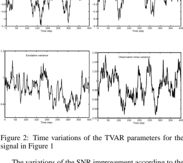
However, in another experiment, we notice that the crite-rion of the SNR improvement is not relevant to measure the quality of the TVAR estimation. Figure 1 shows 400 samples of the test signal generated by a second-order TVAR process. The corresponding TVAR parameters, depicted in Figure 2, follow a first-order Markov process as defined in section 2.1
with fixed parameters∆a1=∆a2 = 10
−2for the TVAR
coef-ficients andδ2
e =δn2= 10−3for the log-variance.
0 50 100 150 200 250 300 350 400 −15 −10 −5 0 5 10 15 TVAR signal Time step
Figure 1: Time variations of the synthetic second-order TVAR signal 0 50 100 150 200 250 300 350 400 −1.2 −1 −0.8 −0.6 −0.4 −0.2 0 0.2 0.4 0.6 Time step TVAR coefficient: a(1)
0 50 100 150 200 250 300 350 400 −0.8 −0.6 −0.4 −0.2 0 0.2 0.4 0.6 0.8 1 Time step TVAR coefficient: a(2)
0 50 100 150 200 250 300 350 400 0.8 1 1.2 Time step Excitation variance 0 50 100 150 200 250 300 350 400 0.92 0.94 0.96 0.98 1 1.02 1.04 1.06 Time step Observation noise variance
Figure 2: Time variations of the TVAR parameters for the signal in Figure 1
The variations of the SNR improvement according to the input SNR are shown in Figure 3. They were obtained by a single run of the algorithm for each value of the input SNR, using 500 particles. The use of a single run is allowed by the small variance of the results when using 500 particles, as shown in [1].
The SNR improvement decreases as the input SNR in-creases, whereas the cepstral distance dein-creases, indicating a better model estimation. One could suggest to take simply
−10 −5 0 5 10 15 20 25 30 35 40 −20 −10 0 10 20 30 40 SNR input (dB)
Cepstral distance (scaled) SNR improvment (scaled) SNR output
Figure 3: SNR improvement, output SNR and cepstral dis-tance.
the SNR output as a measure of the quality but its growth does not match the decrease of the cepstral distance: the lat-ter stops decreasing from input SNR = 20 dB while the output SNR goes on increasing.
Another drawback of the SNR criterion is its dependence on the denoising phase: what is evaluated is not the quality of the TVAR estimation but the quality of the denoising using this estimation.
At last, such a criterion implies that the original signal x is available, which is not realistic for a natural signal.
3.3 Conventional statistical approach for model ade-quacy
Let Y1, ...YN be the random variables associated to the
obser-vations y1, ..yt. If the model is correct, the sequence
ut= p(Yt≤ yt|y1:t−1) (9) is a realization of an independent random variable uniformly distributed on [0, 1]. By letting the time series vt=φ−1(ut),
whereφis the standard normal cumulative distribution
func-tion, the TVAR model is correct if vt is i.i.d according to
N (0, 1) [1].
According to [1], the computing of the ut requires
in-tegration over the model parameters. The latter is approxi-mated by a Monte Carlo estimation using the particle filter.
Therefore, an estimate of ut is given by:
ˆ ut, 1 N N
∑
i=1 p(Yt≤ yt|θ1:t(i), y1:t−1), (10)whereθt(i)is the i-th particle at time t.
The statistical tests employed here aim at testing the
nor-mality and the whiteness of the time series vt and are briefly
described below:
Whiteness
We measure the correlation by a whiteness index given by the Ljung-Box test. This index is defined by:
qLBK = N(N + 2) K
∑
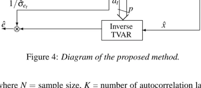
i=1 ˆr2i (N − i), (11) Kalman filter e ¾ e - -e - Particle filter ? ? b e ? 1/ ˆσet ˆ e at p σet x ˆ x ˆ at p y -Inverse TVAR ¾ ¾ TVARFigure 4: Diagram of the proposed method.
where N = sample size, K = number of autocorrelation lags and ˆri denotes the ithautocorrelation coefficient of the time
series. For a white signal, qLBk is asymptotically Chi-Square
distributed.
Normality
The Bowman-Shenton test evaluates the hypothesis that the time series has a normal distribution. The test is based
on the skewnessγ1= µ3
µ2(3/2)
and kurtosisγ2= µ4
µ2(2)
− 3 of the
time series, with µi the ith central moment of the random
variable associated with the time series around its mean µ.
The statistic value associated to this test is given by:
qBS=γ12+γ22. (12)
For a true gaussian distribution, the statistic qBS should be
closer to 0.
4. PROPOSED APPROACH
Assuming that a signal x is produced by a TVAR system ex-cited by a stationary gaussian white noise, the estimation is good if there exists a stationary gaussian white noise that can produce x by exciting the estimated TVAR model. The pro-posed method is then based on the evaluation of the statistical properties of the estimated excitation, ˆe(t), that can generates
the TVAR signal x(n). Indeed ˆe(t), which is defined by
ˆ e(t) = 1 ˆ σet µ x(t) − p
∑
i=1 ˆ ai,tx(t − i) ¶ , (13)must be stationary, white and gaussian. Note that ˆa =
( ˆai,t, ..., ˆap,t) is the vector of estimated TVAR coefficients and
ˆ
σet corresponds to the estimated variance of the TVAR
inno-vation sequence.
Since the original signal x is not available for natural sig-nals under noisy observation, we replace it by the estimated
signal ˆx, given by the Kalman filter. With this approximation,
an estimation for the excitation may be defined as follows:
ˆ e(t) = 1 ˆ σet µ ˆ x(t) − p
∑
i=1 ˆ ai,tx(t − i)ˆ ¶ . (14)According to (14), the principle of the method can be then illustrated with a diagram (see Figure 4).
Besides the normality and whiteness that are classically evaluated, we have introduced the assessment of the esti-mated excitation stationarity. Indeed, the stationarity crite-rion is all the more crucial since the original TVAR signal is non stationary.
Stationarity
The method we choose to detect non stationarity is based on the stationarity index used in [5], which is the Kol-mogorov distance between the time frequency representa-tions (TFR) of the signal at different times. The latter is given by: SI(n) = Z p τ=0 Z +∞ f =−∞ |NI1(n;τ, f ) − NI2(n;τ, f )|d f dτ. (15)
NI1(n;τ, f ) and NI2(n;τ, f ) represent a normalization of re-spectively subimages I1(n;τ, f ) and I2(n;τ, f ):
NIk(n;τ, f ) = |Ik(n;τ, f )| Rp τ=0 R+∞ f =−∞|Ik(n;τ, f )|d f dτ , (16) where the two subimages I1(n;τ; f ) and I1(n;τ; f ) with equal duration p are extracted from the global TFR on both sides of instant n:
I1(n;τ, f ) = T FR(n − p +τ, f ); (17)
I2(n;τ, f ) = T FR(n +τ, f ). (18) The parameter p delimits the considered analysis du-ration at each instant n and allows the selectivity/sensivity control of the SIs: higher p lead to smoother SIs. As used in [4], we fixed p to 20.
We propose to measure the stationarity of the estimated excitation ˆe by the variance of its stationarity index. To
eval-uate the normality and the whiteness of ˆe, we use the
respec-tive criteria presented in section 3.3.
5. EXPERIMENTAL RESULTS
The experiments aim at validating our approach and compare it to the one presented in subsection 3.3. Thus, we propose to study the correlation between the cepstral distance and the statistical criteria performed on both residual time series v as
defined in subsection 3.3 and the estimated excitation ˆe.
The test signal is a synthetic TVAR signal of order 2 (see
Figure 1), with∆a= 10−2I2 for the TVAR coefficients and
δ2
e =δn2= 10−3 for the log-variance (see Figure 2). From
Figure 1, one can see that the time variations of the synthetic TVAR signal are similar to those of a natural speech signal.
At a first stage, we investigated the quality of TVAR esti-mation according to the particles’ number N. For each
exper-iment, the time series v and the estimated excitation ˆe were
computed and analyzed using the three statistical tests pre-sented in sections 3.3 and 4. Since the subsection 3.2 stressed the need of a new criterion especially for input SNR > 20 dB, we fixed SNR to 30 dB. The TVAR estimation was per-formed for different values of N.
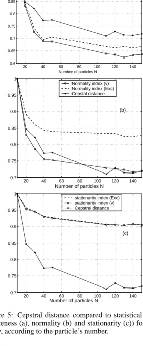
Figure 5 compares the variations, over N, of the standard-ized statistical criteria and the cepstral distance for both time
series v and ˆe. These reported results were obtained by an
averaging over 30 independent runs for each value of N. As expected, the estimation quality is improved by the increase of N: both statistical criteria and cepstral distance decrease as the particles’ number increases up to 100. As a preliminary conclusion, the whiteness, the normality and the stationarity of ˆe and v appear as good indicators of the TVAR estimation quality, since they follow the same evolution as the cepstral distance. 20 40 60 80 100 120 140 0.6 0.65 0.7 0.75 0.8 0.85 0.9 0.95 1 Number of particles N Cepstral distance Whiteness index (v) Whiteness index (Exc)
(a) 20 40 60 80 100 120 140 0.7 0.75 0.8 0.85 0.9 0.95 1 Number of particles N Normality index (v) Normality index (Exc) Cepstal distance (b) 20 40 60 80 100 120 140 0.7 0.75 0.8 0.85 0.9 0.95 1 Number of particles N
stationarity index (Exc) stationarity index (v) Cepstral distance
(c)
Figure 5: Cepstral distance compared to statistical criteria
(whiteness (a), normality (b) and stationarity (c)) for both ˆe
and v, according to the particle’s number.
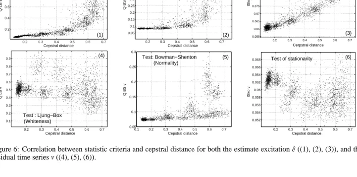
At a second stage, the estimation of the TVAR parame-ters through particle filter was performed for various values of the input SNR (−10 : 2 : 40 dB) and for various values of the particles’ number N (10 : 10 : 150 particles). This simu-lation was repeated 30 times for each pair (SNR, N). Figure 6 shows the correlation of the statistical criteria with the
cep-stral distance for both time series v and ˆe. Each experiment
is represented by a point of coordinates (dC, I) where dC is
the cepstral distance and I refers to one of the three indices (whiteness / normality / stationarity) for v or ˆe.
These reported results demonstrate that the statistical in-dices related to the estimated excitation ˆe are well correlated to the cepstral distance. The correlation degrees depends on the estimation quality . Indeed, for cepstral distances below 0.6, the whiteness, the normality and the stationarity are
al-0.2 0.3 0.4 0.5 0.6 0.7 0.2 0.4 0.6 0.8 1 1.2 Cepstral distance Q LB Exc (1) Test : Ljung−Box (Whiteness) 0.2 0.3 0.4 0.5 0.6 0.7 0.05 0.1 0.15 0.2 0.25 0.3 0.35 0.4 0.45 0.5 0.55 Cepstral distance Q BS Exc Test: Bowman−Shenton (Normality) (2) 0.2 0.3 0.4 0.5 0.6 0.7 0.055 0.06 0.065 0.07 0.075 0.08 0.085 0.09 0.095 0.1 Cepstral distance ISko Exc (3) Cerpstral distance Test of stationarity 0.2 0.3 0.4 0.5 0.6 0.7 0.1 0.2 0.3 0.4 0.5 0.6 0.7 0.8 0.9 Cepstral distance Q LB v Test : Ljung−Box (Whiteness) (4) 0.1 0.2 0.3 0.4 0.5 0.6 0.7 0.05 0.1 0.15 0.2 0.25 0.3 Cepstral distance Q BS v Test: Bowman−Shenton (Normality) (5) 0.2 0.3 0.4 0.5 0.6 0.7 0.052 0.054 0.056 0.058 0.06 0.062 0.064 0.066 0.068 Cepstral distance ISko v Test of stationarity (6)
Figure 6: Correlation between statistic criteria and cepstral distance for both the estimate excitation ˆe ((1), (2), (3)), and the
residual time series v ((4), (5), (6)).
most linearly related to the cepstral distance. Such significant correlation is not observable for v.
To support these results, we computed the correlation co-efficients between the cepstral distance and each criterion. The obtained results, summarized in Table 1, confirm that the proposed approach is more coherent with the cepstral dis-tance than the conventional assessing method (time series v).
Whiteness Normality Stationarity
ˆ
e 0.93 0.6 0.95
v 0.06 0.80 -0.7
Table 1: Correlation coefficients between the statistical crite-ria and the cepstral distance for both the estimated excitation
ˆ
e and the time series v.
The low complexity is another advantage of the proposed method. Whereas the classical validation method based on v, requires the computation of an er f c for each particle, our method requires a simple FIR filtering based on the estimated TVAR model.
6. CONCLUSION
We have shown that the indirect criteria based on the SNR are not relevant for the evaluation of a TVAR estimation. We have proposed a new evaluation method based on the mea-sure of the normality, the stationarity and the whiteness of the estimated excitation. The latter is the output of the in-verse estimated TVAR system.
With a lower complexity than the classical method based on residual time series v, the proposed method leads to better results: the whiteness, normality and stationarity indices are strongly correlated to the cepstral distance between the true and the estimated TVAR models.
Note that the proposed method does not aim at perform-ing a binary validation (valid / not valid). It is thought as a
quantitative measure of the quality of the TVAR model es-timation, which could be used for example to compare two TVAR estimations. In addition, the great advantage of this method is that it does not need any knowledge of the original model, neither of the original signal, contrary to the evalua-tion through SNR criteria.
REFERENCES
[1] J. Vermaak, C. Andrieu, A. Doucet, SJ. Godsill. Parti-cle Methods For Bayesian Modeling And Enhancement Of Speech Signals, IEEE Trans. Speech and Audio Proc, Vol. 10 (3), pp. 173–185, 2002.
[2] M. Sanjeev, S. Maskell, N. Gordon, T. Clapp, A Tutorial On Particle Filters For Online Nonlinear/Non-Gaussian Bayesian Tracking, IEEE Trans. Signal Processing, Vol. 50 (2), pp. 174–188, 2002.
[3] G. Faucon, R. Le Bouquin, A. Akbari, Mesures Objec-tives De La R´eduction De Bruit, GRETSI, Juan les Pins, pp. 587–590, 1993
[4] S. Larbi, M. Jaidane, Audio Watermarking: A Way To Stationarize Audio Signals, IEEE Trans. Signal Process-ing, Vol. 53 (2), pp. 816–823, 2005.
[5] H. Laurent, C. Doncarli Stationarity index for abrupt changes detection in the time-frequency plane, IEEE Signal Processing Letters, Vol. 5, no 2, pp. 43-45, 1998.