The Coloring Game on Planar Graphs with Large Girth, by a result on Sparse Cactuses

HAL Id: hal-01175659

https://hal.archives-ouvertes.fr/hal-01175659

HAL is a multi-disciplinary open access

archive for the deposit and dissemination of sci-entific research documents, whether they are pub-lished or not. The documents may come from teaching and research institutions in France or

L’archive ouverte pluridisciplinaire HAL, est destinée au dépôt et à la diffusion de documents scientifiques de niveau recherche, publiés ou non, émanant des établissements d’enseignement et de recherche français ou étrangers, des laboratoires

The Coloring Game on Planar Graphs with Large Girth,

by a result on Sparse Cactuses

Clément Charpentier

To cite this version:

Clément Charpentier. The Coloring Game on Planar Graphs with Large Girth, by a result on Sparse Cactuses. 2015. �hal-01175659�

The Coloring Game on Planar Graphs with Large Girth,

by a result on Sparse Cactuses

Cl´ement Charpentier∗

Institut Fourier, Universit´e Joseph Fourier, UMR 5582, Grenoble Maths `a Modeler

June 10, 2015

Abstract

We denote by χg(G) the game chromatic number of a graph G, which is the smallest number of colors Alice needs to win the coloring game on G. We know from Montassier et al. [M. Montassier, P. Ossona de Mendez, A. Raspaud and X. Zhu, Decomposing a graph into forests, J. Graph Theory Ser. B, 102(1):38-52, 2012] and, independantly, from Wang and Zhang, [Y. Wang and Q. Zhang. Decomposing a planar graph with girth at least 8 into a forest and a matching, Discrete Maths, 311:844-849, 2011] that planar graphs with girth at least 8 have game chromatic number at most 5.

One can ask if this bound of 5 can be improved for a sufficiently large girth. In this paper, we prove that it cannot. More than that, we prove that there are cactuses CT (i.e. graphs whose edges only belong to at most one cycle each) having χg(CT ) = 5 despite having arbitrary large girth, and even arbitrary large distance between its cycles.

1

Introduction

We only consider in this paper simple, finite, and undirected graphs. The length of a path or cycle is the cardinal of its edge-set. The girth g(G) of a graph G is the length of its smallest cycle. A cactus is a graph G in which any edge belongs to at most one cycle. The cycle-distance of a cactus is the length of its smallest path between two vertices belonging to different cycles. For a vertex v, we call v-leaf a vertex of degree 1 (or leaf ) whose neighbor is v.

The coloring game on a graph G is a two-player non-cooperative game on the vertices of G, introduced by Brams [8] and rediscovered ten years after by Bodlaender [3]. Given a set of k colors, Alice and Bob take turns coloring properly an uncolored vertex, with aim for Alice to color entirely G, and for Bob to prevent Alice from winning. The

∗

This research is supported by the ANR project GAG (Games and graphs), ANR-14-CE25-0006, 2015-2018.

Figure 1: A cactus with game chromatic number 5 [13]

game chromatic number χg(G) of G is the smallest number of colors insuring Alice’s

victory. This graph invariant has been extensively studied these past twenty years, see for example [9, 12, 16, 17].

In [3], Bodlaender proved that every forest F has χg(F ) ≤ 5, and exhibited trees

T with χg(T ) ≥ 4. In [7], Faigle et al. showed that every forest F has χg(F ) ≤ 4.

Conditions for trees to have game chromatic number 3 were recently studied by Dunn et al. [6].

A graph is said (1, k)-decomposable if its edge set can be partitionned into two sets, one inducing a forest and the other inducing a graph with maximum degree at most k. Using the notion of marking game introduced by Zhu in [15], He et al. observed in [10] that every (1, k)-decomposable graph has χg(G) ≤ k + 4, then deduced upper

bounds for the game chromatic number of planar graphs with given girth. Among other results, they proved that planar graphs with girth at least 11 are (1, 1)-decomposable, and therefore their game chromatic number is at most 5. Later, were proved successively the (1, 1)-decomposability of planar graphs with girth 10 by Bassa et al. [2], girth 9 by Borodin et al. [5], and girth 8 by Montassier et al. [11] and Wang and Zhang [14] independantly. There exist planar graphs with girth 7 that are not (1, 1)-decomposable. Borodin et al. [4] gave conditions for planar graphs with no small cycles except triangles to be (1, 1)-decomposable, in terms of distance between the triangles and of minimal length of a non-triangle cycle. In [13], Sidorowicz, arguing that cactuses are (1, 1)-decomposable, showed that every cactus CT has χg(CT ) ≤ 5. Moreover, she

exhibited a cactus with game chromatic number 5, depicted in Figure 1. As one can see, this cactus has intersecting triangles.

The work we present here started as we tried to answer the following question:

Question 1. Is there an integer g such that every planar graph G with girth at least g has χg(G) ≤ 4 ?

We answer negatively, with a result going way beyond the question we initially asked.

Theorem 1. For any integers d, k, there are cactuses CT with girth at least k, cycle-distance at least d and χg(G) = 5.

This proves that the upper bound of 5 for the game chromatic number of the classes of (1, 1)-decomposable graphs considered in [2, 4, 5, 10, 11, 14] are best possible.

As our construction needs odd cycles, this asks whether or not this result generalizes to bipartite graphs, seeming more difficult to handle. This question is still open. As a

¶ ·

¸ ¹

¶ ¶

¸ ¸

Figure 2: Two winning paths (Lemma 2)

partial result, we can find in [1] a proof by Andres and Hochst¨attler that every forest with thin 4-cycles, which is a cactus constructed from a forest by replacing some edges uv by a pair of 2-vertices both adjacent to u and v (and which is bipartite), has game chromatic number at most 4.

2

Proof of Theorem 1

We consider Alice and Bob playing the coloring game on a graph G with a set of four colors C = {¶,·,¸,¹}. At each time of the game, we denote by φ(v) the color of a vertex v (if v is colored), and by Φ(v) the set of colors in the neighborhood of v: if v is uncolored, then this is the set of colors forbidden for v. We call surrounded an uncolored vertex v with Φ(v) = C. Bob wins if he can surround a vertex.

We give further the construction of G. For now just assume that every cycle of G is odd and that every non-leaf vertex of G is adjacent to a large number of leaves, say at least 8 leaves.

We also give further Bob’s strategy in details, but assume that Bob only plays on the leaves of G. Also, for any vertex v, when Bob colors a v-leaf, he uses a color that is not already in Φ(v). If Alice colors a v-leaf during the game, then Bob always colors another v-leaf if possible. So we can assume that for any uncolored vertex v, there is always at least one uncolored leaf of v. Moreover, coloring a v-leaf for Alice does not suppress any possibility for Bob (this forbid Bob to color v with the color Alice used, but Bob had no intention to color v anyway) and only increase Φ(v), coloring a leaf is always unoptimal for Alice. So we assume Alice never colors a leaf during the game.

We describe some winning positions for Bob (i.e. partial colorings from where Bob has a winning strategy) in the following lemmas. In the description of every winning position, we assume that it is Alice’s turn to play.

Lemma 2. Suppose that G contains a path of length d, P = v0. . . vd, of uncolored

non-leaf vertices. Also suppose |Φ(v0)| ≥ 2, say {¶,¸} ⊆ Φ(v0). The game is in a winning

position for Bob if (see Figure 2):

• d is odd and {¶,¸} ⊆ Φ(vd).

We say that P is a winning path.

Proof. Recall that, by assumption, every vertex of P has at least one uncolored leaf. In the case d = 0, P is reduced to a single surrounded vertex and Bob wins.

The case d = 1 corresponds to an edge v0v1 with v0 and v1 uncolored and |Φ(v0) ∩

Φ(v1)| ≥ 2, say {¶,¸} ⊆ Φ(v0) ∩ Φ(v1). If Alice colors v0, she has to use an even color,

Bob colors a v1-leaf with the other even color, surrounds v1, and wins. If Alice colors

v1, then Bob can surrounds v0 as well. So Bob’s winning strategy consists in coloring

leaves of v0 with different colors until v0 is surrounded or Alice colors v0 or v1.

We prove the other cases by induction. Assume that our lemma is true for every value of d strictly smaller than an integer q and consider the case d = q. Bob’s strategy is to colors a v0-leaf until v0 is surrounded or Alice colors a vertex of P . When Alice

colors a vertex vi of P , we consider two cases.

• If i = 0 or i = q, say w.l.o.g. i = 0, then she uses an even color. Bob colors a v1-leaf with the other even color. By induction, Bob wins since P − v0 is a winning

path of length q − 1.

• If i 6= 0 and i 6= q, then let P1 = v0. . . vi−1 and P2 = vi+1. . . vq. We denote by d1

and d2 the length of P1 and P2 respectively. We have d1+ d2= q − 2. We consider

two subcases:

– Either q is even, and d1 and d2 are either both even or both odd. Say we have

{¶,¸} ⊆ Φ(v0) and {·,¹} ⊆ Φ(vq). Without loss of generality, assume Alice

colored vi with¶. If d1and d2 are both odd, then Bob colors a vi−1-leaf with

¸. If they are both even, then Bob colors a vi+1-leaf with ¸. Path P1 or P2

respectively is a winning path and Bob wins by induction hypothesis. – Either q is odd, and say {¶,¸} ⊆ Φ(v0) ∩ Φ(v1). Among d1 and d2, one is

even and one is odd, say d1 is even and d2 is odd. If Alice colored vi with

an odd color, then Bob colors a vi+1-leaf with the other odd color. If Alice

colored vi with an even color, then Bob colors a vi−1-leaf with the other even

color. Path P1or P2 respectively is a winning path and Bob wins by induction

hypothesis.

This concludes our proof.

Lemma 3. Suppose that C is an (odd) cycle of G of uncolored vertices. If there are two neighbors u and v with |Φ(u)| ≥ 2 and |Φ(u) ∩ Φ(v)| = 1 (see Figure 3), then G is in a winning position for Bob. We say that C is a winning cycle.

Proof. Let C = v0v1. . . vkbe an odd cycle of uncolored vertices with, say, {¶,·} ⊆ Φ(v0)

and¶ ∈ Φ(v1). If the next Alice’s move is not to color v0 or v1, then Bob colors a leaf of

v1 with· and Bob wins by Lemma 2 (v0v1 is a winning path). If Alice colors v0, then

she has to use a color different to ¶ and, at his turn, Bob colors a vk-leaf with¶. Since

¶ ¸

¶

Figure 3: A winning cycle (Lemma 3)

¶ ¸

·

Figure 4: A winning cycle-path (Lemma 4)

Alice colors v1, Bob can color a v2-leaf with a color among¶ and · different from φ(v1)

and v2. . . vkv0 is a winning path.

Lemma 4. Suppose that G contains a path of length d, P = v0. . . vd, of uncolored

non-leaf vertices. Also suppose |Φ(v0)| ≥ 2, say {¶,¸} ⊆ Φ(v0), and suppose vd belongs to

an odd cycle C of uncolored vertices, with w being a neighbor of vd in this cycle. Graph

G is in a winning position for Bob if (see Figure 4): • d is even and ¶ or ¸ is in Φ(w).

• d is odd and · or ¹ is in Φ(w). We say that P ∪ C is a winning cycle-path.

Proof. The case d = 0 is true by Lemma 3, since C is then a winning cycle.

We prove the other cases by induction on d. Assume our lemma is true for every value of d strictly smaller than q. We consider the case d = q. We have different cases depending of Alice’s move:

• If Alice colors w, then let w0 be the neighbor of w different from vq. The uncolored

vertices of P ∪ C form a path P0 = v0, . . . , vq, . . . , w0. Since C has odd length, one

path among P and P0 is odd and the other is even. If φ(w) ∈ Φ(v0), then Bob can

color a leaf of vq or w0 such that the odd path among P and P0 become a winning

path. If φ(w) 6∈ Φ(v0), then Bob colors a leaf of vq or w0 such that the even path

among P and P0 is a winning path. By Lemma 2, Bob is winning the game.

• If Alice colors v0, then Alice has to use an even color, Bob colors a v1-leaf with the

other even color and (P − v0) ∪ C is a winning cycle-path, Bob wins by induction

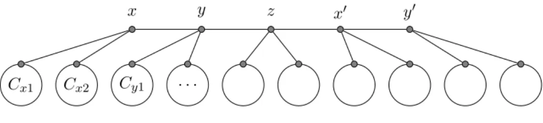
x y z _x0 _y0

Cx1 Cx2 Cy1 . . .

Figure 5: A sketch of graph G

• If Alice colors v_q, then let w00 be the other neighbor of vd in C than w. If there

is in Φ(w) a color c different to φ(vq), then Bob colors w00 with c and C − vd is

winning path since C has odd length. By Lemma 2, Bob wins. If Φ(w) = φ(vd),

then we have two cases:

– If d is even, then φ(vd) = ¶ or ¸, say ¶. Bob colors a vd−1-leaf with¸ and

P − vdis a winning path.

– If d is odd, then φ(vd) = · or ¹, say ·. Bob colors a vd−1-leaf with ¹ and

P − vdis a winning path.

Bob wins by Lemma 2.

• If Alice colors vi, i 6= 0 and i 6= q, then let P1= v0. . . vi−1and P2 = vi+1. . . vq. We

denote by d1and d2 the length of P1 and P2 respectively. We have d1+ d2 = q − 2.

We consider two subcases:

– If d1 is odd and Alice used an odd color on vi, or if d1 is even and Alice used

an even color on vi, then Bob colors vi−1 with the other odd color (resp. the

other even color), and Bob wins by Lemma 2 (P1 is a winning path).

– If d1 is odd and Alice used an even color on vi, or if d1 is even and Alice used

an odd color on vi, then Bob colors vi+1 with the other even color (resp. the

other odd color). Bob wins by induction hypothesis, since P2∪ C is a winning

cycle-path of smaller path-length.

• If Alice colors another vertex, then one can observe that Bob can color a w-leaf in such a way that P + w is a winning path.

Our lemma is true for every d by induction. This concludes our proof.

Corollary 5. If, at Bob’s turn, there is in G an uncolored path P = v0, . . . , vd such that

|Φ(v0)| ≥ 2 and vd belongs to an uncolored odd cycle, then Bob has a winning strategy

(he can obtain a winning cycle-path in one move).

We describe now explicitely the graph G on which Alice and Bob are playing, depicted in Figure 5. Here paths and cycles have arbitrary large length and cycles are odd. For a vertex v, we say we attach a cycle C to v with a path P if we add C and P such that the endvertices of P are v and a vertex of C. We start from a path xyzy0x0, then for

every vertex v in this path, we attach two odd cycles Cv1 and Cv2 to v with two paths

Pv1 and Pv2 respectively. We denote Gv = Cv1+ Cv2+ Pv1+ Pv2. Finally, we copy our

graph (i.e. we add a similar second connected component to the graph). Then we add a large number of leaves (at least 8) to every vertex to obtain G.

Now we give the winning strategy for Bob. As we assumed, Bob only plays on leaves. After Alice’s first move, Bob considers the connected component of the graph where Alice did not play on and will only play on it.

Step 1. Bob plays in Gz. He aims to end Step 1 with his victory or with Alice coloring

z. Moreover, Bob wants to be sure Alice colors in Step 1 at most one vertex not in Gz.

At his first move, Bob colors a z-leaf with an arbitrary color. If Alice colors z at her second move, then Bob goes to Step 2. Otherwise, Bob colors another z-leaf with another color. If Alice colors z, then Alice played at most one move out of Gz and Bob goes to Step 2. Otherwise,

• If Alice has played her two moves in G_z, then Bob colors another z-leaf and Alice has to color z for Bob not to surround it next turn. Bob goes to Step 2. • Otherwise, then we can assume without loss of generality that Pz1∪ Cz1 is

uncolored, and Bob wins by Corollary 5.

Step 2. Since Alice only played once out of Gz, we assume that Gx∪ Gy is uncolored.

Now Bob plays in Gx. He aims to end Step 2 with his victory or with Alice coloring

x with a color different from φ(z). Moreover, Bob wants to be sure Alice colors in Step 2 at most one vertex not in Gx, and this vertex, if it exists, is not y.

Step 2 is quite similar to Step 1. Bob begins by coloring a x-leaf with φ(z). If Alice colors y, she has to use a color different from φ(z) and Bob wins by Corollary 5. If she colors x, then Bob goes to Step 3. If she colors any other vertex, then Bob colors another x-leaf, and, from this point, this is similar to Step 1.

Step 3. We can assume without loss of generality that Py1∪ Cy1 is uncolored. Since

|Φ(y)| ≥ 2, Bob wins by Corollary 5.

This ends the proof of Theorem 1.

References

[1] S.D. Andres and W. Hochst¨attler. The game chromatic number and the game colouring number of classes of oriented cactuses. Information Processing Letter, 111:222–226, 2011.

[2] A. Bassa, J. Burns, J. Campbell, A. Deshpande, J. Farley, M. Halsey, S. Micha-lakis, P.-O. Persson, P. Pylyavskyy, L. Rademacher, A. Riehl, M. Rios, J. Samuel, B. Tenner, A. Vijayasaraty, L. Zhao, and D.J. Kleitman. Partitionning a planar graph of girth ten into a forest and a matching. (manuscript), 2004.

[3] H. L. Bodlaender. On the complexity of some coloring games. Inter. J. of Found. Computer Science, 2(2):133–147, 1991.

[4] O. V. Borodin, A. O. Ivanova, A. V. Kostochka, and N. N. Sheikh. Planar graphs decomposable into a forest and a matching. Discrete Math., 309:277–279, 2009.

[5] O. V. Borodin, A. V. Kostochka, N. N. Sheikh, and G. Yu. Decomposing a planar graph with girth 9 into a forest and a matching. Europ. J. of Comb., 29:1235–1241, 2008.

[6] C. Dunn, V. Larsen, K. Lindke, T. Retter, and D. Toci. The game chromatic number of trees and forests. 2014. (Submitted).

[7] U. Faigle, W. Kern, H.A. Kierstead, and W.T. Trotter. On the game chromatic number of some classes of graphs. Ars Combin., 35:143–158, 1993.

[8] M. Gardner. Mathematical game. Scientific American, 23, 1981.

[9] D. Guan and X. Zhu. The game chromatic number of outerplanar graphs. J. Graph Theory, 30:67–70, 1999.

[10] W. He, X. Hou, K.-W. Lih, J. Shao, W.-F. Wang, and X. Zhu. Edge-partitions of planar graphs and their game coloring numbers. J. Graph Theory, 41(4):307–317, 2002.

[11] M. Montassier, P. Ossona de Mendez, A. Raspaud, and X. Zhu. Decomposing a graph into forests. J. Combin. Theory Ser. B, 102(1):38–52, 2012.

[12] A. Raspaud and J. Wu. Game chromatic number of toroidal grids. Information Processing Letters, 109:1183–1186, 1999.

[13] E. Sidorowicz. The game chromatic number and the game colouring number of cactuses. Information Processing Letters, 102:147–151, 2007.

[14] Y. Wang and Q. Zhang. Decomposing a planar graph with girth at least 8 into a forest and a matching. Discrete Math., 311:844–849, 2011.

[15] X. Zhu. The game coloring number of planar graphs. J. Combin. Theory Ser. B, 75(2):245–258, 1999.

[16] X. Zhu. Game coloring number of pseudo partial k-trees. Discrete Maths, 215:243– 262, 2000.

[17] X. Zhu. Refined activation strategy for the marking game. J. Combin. Theory Ser. B, 98(1):1–18, 2008.