Coordinating inventory control and pricing strategies

(1)

Coordinating Inventory Control and Pricing

Strategies

by

Xin

Chen

B.S., Computational Mathematics

(1995)

Xiangt an University

M.S., Computational Mathemat'ics (1998)

Chinese Academy of Sciences

Submitted t o the Sloan School of Management

in partial fulfillment of tjhe requirements for the degree of

Doctor of Philosophy in Operations Research

OF TECHNOLOGY

a t the

MASSACHUSETTS INSTITUTE O F TECHNOLOGY

June 2003

@

Massachusetts Institute of Technology 2003. All rights reserved.

. . .

Author

Sloan School of Management

May

16,

2003

Certified by.

. . .

.D!,.

d

. . . .

.5

:. ?

. . .

David Simchi-Levi

Professor

of

Engineering Systems

Thesis Supervisor

Accepted b y . .

. . .

John N. Tsitsiklis

Professor of Electrical Engineering and Computer Sciences

Co-Director, Operations Research Center

(2)

(3)

Coordinating Inventory Control

and

Pricing Strategies

Xin Chen

Submitted to tlhe Sloan School of Management on May 16, 2003, in partial fulfillment of the

requirements for the degree of

Doctor of Philosophy in Operations Research

Abstract

Traditional inventory models focus on effective replenishment stra'tegies and tjypically assume that a commodity's price is exogenously determined. In recent years, however, a number of industries have used innovative pricing stmtegies to manage their inventory effectively. These developments call for models that integrat,e inventory control and pricing strategies. Such models are clea8rly important not only in the retail industry, where price-dependent demand plays an important role, but also in mmufacturing environments in which product~ion/distribution decisions can be com- plemented with pricing strategies to improve the firm's bottom line.

To date, the lit,erat,ure has confined itself mainly t o models with va,riable ordering costs but no fixed costs. Extending some of these models to include a fixed cost component is the main focus of this thesis.

In this thesis, we start by a,nalyzing a single product, periodic review joint inventory control and pricing model, and characterizing the ~ t ~ r u c t u r e of the optimal policy under various conditions. Specificall;y, for the finite horizon periodic review case, we show, by employing the classical k-convexity concept, that a simple policy, called (s, S, p), is optimal when the demand functions are additive. For the model with more general demand functions, we show that an (s,

S,

p) policy is not necesmrily optimal. We introduce a new concept, the symmetric k-convex functions, and apply it t o provide a characterization of the optima,l policy. Surprisingly, in the infinite horizon periodic review case, the concept of symmetric k-convex functions allows us to show tha,t a stationary (s,

5';

p) policy is optimal for both discounted and average profit models even for general demand functions. Our approach developed for the infinite horizon periodic review joint inventory control and pricing problem is then extended to a corresponding continuous review model. In this case, we prove that a stationary ( s , S , p) policy is optimal under fairly general assumptions. Finally, the symmetric k-convexity concept developed in this thesis is employed to characterize the optimal policy for the stochastic cash balance problem.

(4)

Thesis Supervisor: David Simchi-Levi Title: Professor of Engineering Systems

(5)

Acknowledgments

I am indebted to my thesis advisor Professor David Simchi-Levi for guiding me on this exciting research. His wisdom greatly shaped my thinking and this thesis. Besides research, David also gave me help in many aspects of my life. I cannot imagine how my life would have been without him. Any knowledgement cannot express my gratitude t o David. In a word, I really enjoy being his student and working closely with him. His supervision is my best experience at MIT.

My thesis committee members, Professor Stephen Graves and Professor John Tsistsiklis, provided insightful comments and suggestions on this research. Their input is highly appreciated. Professor Paul Tseng a t the University of Washington gave me support and help by being an advisor and a friend when I was studying there.

I

am very grateful for everything he has done for me. My master thesis advisor, Professor Yaxiang Yuan a t the Chinese Academy of Sciences, has been my source of inspiration for pursuing high-level research.

ORC was a great place. I sincerely appreciate ORC for giving me the opportunity to study toward my PhD. Professor James Orlin, Professor Robert Freund, Professor Charles Fine and Professor Georgia Perakis provided me with their support and suggestions. The administrative staff at ORC also gave me a lot of help.

I would like to thank my friends at MIT, mostly at ORC, for making my life really enjoyable: Opher Baron, Damian Beil, Su Shen, Yong Shi, Ping Xu,

...,

just to name a few. In particular, it is very fortunate to have Melvyn Sim and Peng Sun as very good friends. In the past years, they have given me support and haved shared my happiness and hardships. My life would never have been the same without them.

Finally, I am indebted to my family for their support. My parents and my brother are always supportive for my studies faraway from home. My wife Yu Sheng gives me endless support, encouragement and love during ups and downs. This thesis could not have been finished without her support. My little baby Jennifer brings a lot of joy to my life and she is my biggest accomplishment at MIT.

(6)

(7)

List

of Figures

. . .

2-1 Sequence of Events for the Joint Inventory and Pricing Problem 19

2-2 An Example for k-convex Function . . . 26

2-3 An Example for Symmetric k-convex Function . . . 27

2-4 A Two Periods Joint Inventory and Pricing Example

. . .

38

2-5 The Non-Monotonicity of the Price

. . .

38

4-1 The Impact of Inventory HoIding and Short.age Cost . . . 97

4-2 The Impact of Inventory Holding and Shortage Cost . . . 98

4-3 The Impact of Fixed Ordering Cost . . . 98

4-4 The Impact of Demand Uncertainty

. . .

99

(10)

(11)

Chapter

1 Introduction

1 1

Motivations

Tradit,ional inventory models focus on effective replenishment ~trat~egies and typically assume that a c~mmodit~y's price is exogenously determined. In recent years, however, scores of retail and manufacturing companies have startjed exploring innovative pricing strategies in an effort to improve their operations and ultimately tjhe bottom line. Firms a,re employing methods such as dynamica,lly adjusting price over time based on inventory levels or production schedules as well as segmenting customers based on their sensitivity to price and lead time.

For instance, no company underscores t,he impact of the Internet on product pricing strategies more than Dell Computers. The exact same product is sold at different prices on Dell's Web site, depending on whether the purchase is made by a private consumer, a, small, medium or large business, t,he federal government,, an e,ducation or health care provider. A more careful review of Dell's stmtegy, see [I], suggests that even the price of the same product for the same industry is not fixed; it may change significantly over time.

Dell is not alone in its use of a sophisticated pricing strategy. Consider:

(12)

that prices for the 12,000 items ordered most frequently on-line might change as often as daily. [16].

Ford Motor Co. uses pricing strategies to match supply and demand and target particular customer segments. Ford executives credit the effort with $3 billion in growth between 1995 and 1999. [18].

These developments call for models that integrate production decisions, inventory control and pricing strategies. Such models and strategies have the potential to radically improve supply chain efficiencies in much the same way as revenue manage- ment has changed the airline industry, see Belobaba [3] or McGill and van Ryzin [19]. Indeed, in the airline industry, revenue management provided growth and increased revenue by 5%, see Belobaba. In fact, if it were not for the combined contributions of revenue management and airline schedule planning systems, American Airlines (Cook [7]) would have been profitable only one year in the decade beginning in 1990. In the retail industry, to name another example, dynamically pricing commodities can provide significant improvements in profitability, as shown by Gallego and van Ryzin [121s

1.2 Background

The coordination of replenishment strategies and pricing policies has been the focus of many papers, starting with the work of Whitin [28] who analyzed the celebrated newsvendor problem with price dependent demand. For a review, the reader is referred to Eliashberg and Steinberg [8], Petruzzi and Dada 1211, Federgruen and Heching [lo] or Chan, Simchi-Levi and Swann [6].

Federgruen and Heching [lo] investigate a periodic review, single product model with stochastic, price-dependent demand. The authors assume that the demand is a linear function of the selling price, and ordering cost is proportional to the amount ordered and thus does not include a fixed cost component. Under some technical

(13)

assumptions, they show that in this case a base-stock lzst pnce policy is optimal. That is, in each period the optimal policy is characterized by an order-upto level, referred to as the base-stock level, and a price which depends on the initial inventory level at the beginning of the period. If the initial inventory level is below the base- stock level an order is placed to raise the inventory level t o t,he base-stock level. Otherwise, no order is placed and a discount price is offered. This discount price is a non-increasing function of the initial inventory level.

The paper by Thomas [26] considers a model similar to Federgruen and Heching [lo], namely, a periodic review, finite horizon model with a stochastic, price-dependent demand. One significant difference between Thomas [26] and Federgruen and Heching [lo] is that Thomas [26] assumes that the ordering cost includes both a fixed component and a variable component. Thomas provides many negative results regarding the structure of the optimal policy and proposes a simple heuristic, referred t o by Thomas as ( s , S, p), which can be described as follows. The inventory strategy is an (s, S ) policy: If the inventory level at the beginning of period

t

is below the reorder point, s t , an order is placed t o raise the inventory level to the order-upto level, St.

Otherwise, no order is placed. Price depends on the initial inventory level at the beginning of the period. Thomas provides a counterexample which shows that with a "few prices" (i.e., when price is restricted to a discrete set) this policy may fail to be optimal. Thomas goes on t o say:

If all prices in an interval are under consideration, it is conjectured that a n (s, S, p) policy is optimal under fairly general conditions.

1.3 Contributions

To date, the literature has confined itself mainly to the joint inventory control and pricing models with variable ordering costs but no fmed ordering costs. In particular, the structure of the optimal policy for the joint invent,ory control and pricing model

(14)

with a fixed ordering cost has been open since Thomas's paper in 1974. This is exactly t,he starting point of our work.

Specifically, we start with a periodic review, single product model with stochastic demand. Demands in different periods are independent of each other and their distri- butions depend on the product price. Pricing and ordering decisions are made at the beginning of each period, and all shortages are backlogged. The ordering cost includes both a fixed cost and a variable cost proportional t o the amount ordered. Inventtory holding and shortage costs are convex funct,ions of the inventory level carried over from one period to the next. We consider both the finite and infinite horizon models. In the finite horizon model the objective is t o find an inventory policy and a pricing strategy maximizing expected discounted profit over the finite horizon. In the infinite horizon the objective is to maximize expected discounted, or expected average profit. This is followed by a study of a corresponding infi~iit~e horizon continuous review joint inventory control and pricing model. Finally, we study the ~t~ochastic cash balance problem by employing techniques similar t o the one developed for the joint inventory control and pricing problem.

In the following, we summarize the main contributions of this thesis.

(1) In Chapter 2, we analyze a finite horizon periodic review joint inventory control and pricing problem. We prove that an ( s , S, p) policy is indeed optimal when the demand process is additive based on the famous k-convexity concept. Thus, this result proves the conjecture of Thomas [26] for the additive demand model.

To deal with the general demand model, we int,roduce an innovative concept, symmetric k-convexity, and employ it to prove that an (s, S , A , p) policy is optimal. In such a policy, at each time period t , there exists two parameters s t and St and a set At E [st, (st

+

St)/2] such that if the initial inventory level at t,he beginning of time period t is below st or belongs to the set At, an order is placed t o raise the inventory level to St; otherwise, no order is placed. The selling price of time period t is a function of the initial inventory level at time

(15)

period

t .

(2) In Chapter 3, we analyze a corresponding infinite horizon periodic review joint inventory control and pricing problem where all input parameters are stationary. Contrary to the finite horizon model, we prove that in this case, a stationary (s, S, p) policy is optimal even for general demand functions. This is done by employing the symmetric k-convexity concept. We also provide some charac- terizations of the optimal (s, S ) inventory policy.

(3) In Chapter 4, we extend our approach developed for t.he infinite horizon periodic review joint inventory control and pricing problem to a corresponding continuous review model. In particular, we prove that a stationary (s, S , p)

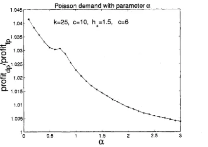
inventory policy is optimal under fairly general assumptions. In addition, we present preliminary computational results illustrating the benefit of ampplying the optimal policy relative to a fixed price policy.

(4) In Chapter 5 , we employ the symmetric k-convexity concept to analyze the stochastic cash balance problem. This problem is a cost minimization problem faced by a firm, which has to decide how much cash to hold in order t,o meet its transaction requirements for a given planning horizon. In this problem, the firm may choose t o increase or decrease the cash levels, which is similar to a stochastic inventory control problem with returns. It turns out that the symmetric k-convexit,y concept developed in our research provides a very natural tool for this problem as well.

The organization of the thesis is as follows. In Chapter 2, we introduce and an- alyze the finite horizon periodic review joint inventory control and pricing model. In Chapter 3, we analyze the infinite horizon case. In Chapt,er 4, we study a cor- responding infinite horizon continuous review model. In Chapter 5 , we apply the

(16)

Chapter 6, we summarize our main results in this thesis and propose some further research directions.

(17)

Chapter

2 Finite Horizon Periodic Review

Model

In this chapter, we focus on a single product, periodic review, finite horizon model. We review the main assumptions of the finite horizon model in Section 2.1. In Section 2.2 we review the concept of k-convexity and introduce a weaker definition of k- convexity, referred t o as symmetric k-convexity. We analyze the finite horizon models with additive demand functions in Section 2.3 and with general demand functions in Section 2.4. In Section 2.5 we in~estigat~e a special case, the finite horizon model with zero fixed ordering cost. FinaIly, we discuss some extensions in Section 2.6.

2.1 TheModel

Consider a firm that has t o make replenishment and pricing decisions over a finite time horizon with

T

periods. For convenience, in t,his case, we index periods from 1 to T where 1 is the last period and T is the first period of the planning horizon.

Demands in different periods are independent of each other. For each period t , t = 1 , 2 . . . , T, let

(18)

pi = selling price in period

t

p -t

,

pt

are lower and upper bounds on pt, respectively.

Throughout Chapter 2 and Chapter 3, we concentrate on demand functions of the following forms:

Assumption 2.1 For t = 1 , 2 , . . .

,

T , the demand function satisfies

where et = ( a t ,

,&),

and a t ,

pt

are two random vamables with E { a t ) = 1 and E { P t ) = 0. The random perturbation,^, ~ t , are .Independent across time. Furthermore, Dt(pt)

is a strict19 decreasing function of pi.

Observe that, by scaling a8nd shifting, the assumptions E { a t ) = 1 and E { & ) = 0 can be made without loss of generality. A special case of this demand function is the additive demand function. In this case, the demand function is of the form

dt = D t ( p )

+

pt.

This implies that only

Pt

is a random variable while at = 1. Another special case of the demand function (2.1) is a model with multiplicative demand. In this case, the demand function is of the form dt = a t D t ( p ) , where at is a random variable. Finally observe that special cases of t,he function D t ( p ) include Dt(p) =

bt - atp (at

>

0 , bt

>

0) in the additive case and D t ( p ) = atpPbt (at

>

0, bt

>

1) in the multiplicative case; both are common in the economics lit,erature (see [21]).

Let

xt

be the inventory level a t the beginning of period t , just before placing an order. Similarly, yt is the inventory level at the beginning of period t aft,er placing an order. The ordering cost function includes both a fixed cost and a variable cost and is calculated for every t , t = 1 , 2 , . .

.,

as

where

1, i f u > O , b(u) :=

(19)

Lead time is assumed to be zero and hence an order placed at the beginning of period

t

arrives immediately before demand for the period is realized.

Unsatisfied demand is backlogged. Let x be the inventory level carried over from period t to the next period. Since we allow backlogging, x may be positive or negative. A cost ht(z) is incurred at the end of period t which represents inventory holding cost when x

>

0 and shortage cost if

x

<

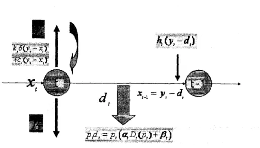
0. Figure 2-1 summarizes the sequence of events of this problem.

Figure 2-1: Sequence of Events for the Joint Inventory and Pricing Problem

Given a discount factor

y

with 0

<

y

5

I, an initial inventory level, XT, and a pricing and replenishment policy, let

(20)

be the T-period total expected discounted profit, where xt-1 = yt - Dt(pt, et). The objective is to decide on ordering and pricing policies so as to maximize total expected discounted profit over the entire pla,nning horizon, that is t,he objectfive is to maximize V ' for any initial inventory level XT and any 0

<

y

5

1.

To find the optimal strategy that maximizes (2.2), let ut(x) be the maximum total expected discounted profit (discounted relative to period

t )

when

t

periods remain in the planning horizon and the inventory level at the beginning of period

t

is x.

A

natural dynamic program that can be applied to find the policy maximizing (2.2) is as follows. For

t

= 1 , 2 , . . .

,

T ,

with vo(x) = 0 for any x , where

For the general demand functions (2.1), we can present the formulation (2.3) only with respect to expected demand rather than with respect to price. Note that there is a one-to-one correspondence between the selling price pt E

[1,

_-t

,

pt] and the expected demand Dt (pi) E

[dt,

&I,

where

We denote the expected demand at period t by d = Dt(p). Also let

where co = 0 and Rt is the expected revenue function with

which is a function of expected demand d. These functions, q&(x)> h l ( y ) and &(d), allow us to transform the original problem to a problem with zero variable ordering cost.

(21)

Specifically, the dynamic program (2.3) can be written as

with q&,(x) = 0 for any x , where

and

ddy) E argmax,,>d,$gt(K d ) . (2.6) Thus, most of our focus is on the transformed problem (2.4) which has a similar structure to problem (2.3). In this transformed problem one can t,hink of hz as being the holding and shortage cost function,

&

as being the revenue function and the variable ordering cost is equal to zero.

For technical reasons, we need the following assumption on the revenue functions as well a3 the holding and shortage cost functions.

Assumption 2.2 For

t

= 1,2, . .

., &

and - ht are concave and as a consequence, the function

is concave. Furthermore, we assume that for any t ,

lim

QT(x)

= -00.

l 4 + ~

Finally, it is appropriate to point out that the fixed cost requires a mild assumption. Indeed, as is customary in traditiond finite horizon i n v e n t o q models, we assume

Assumption 2.3 I n the firrite horizon model with T periods, the j2ed ordering costs satisfy

(22)

2.2 &Convex and Symmetric k-Convex Functions

To motivate the technique used in this research for characterizing the optimal policy under both finite and infinite horizon models, it is useful to relate our problem to the celebrated stochastic inventory control problem discussed by Scarf [24] and Iglehart, [14, 151 for the finite and infinite horizon models, respectively. In that problem

demand is assumed t o be exogenously determined, while in our problem demand depends on price. Other assumptions regarding the framework of the model are similar to those made by Scarf 1241 and Iglehart [14, 151.

For the classical finite horizon stochastic inventory problem Scarf [24] showed

that an (s, S) policy is optimal. In this policy, the optimal decision in period t is characterized by two parameters, the reorder point, st, and the order-up-to level, St. An order of size St - xt is made a t the beginning of period t if the initial inventory level at the beginning of the period, xt, is smaller than st. Otherwise, no order is placed. This results was extended by Iglehart for the infinite horizon case.

To prove that an (s, S ) policy is optimal Scarf [24] uses the concept of k-convexity.

Definition 2.1 A real-valued function f is called k-convex for k

1

0, if for any

z

2

0, b

>

0 and any y we have

A function f is called k-concave zf - f is k-convex.

For the purpose of the analysis of our model, we find it useful t o employ anot,her, yet equivalent,, definition of kconvexityl.

Definition 2.2 A real-valued J;un,ction f is called k-convex for k

2

0, if for any xo 4 X I and X E [ O , l ] ,

f

((1 - +o

+

Xx1)

<

(1 -

X)f

(xo)

+

Xf

(XI)

+

Xk. _(2.9)

'Recently Professor Paul Zipkin pointed out to us that this equivalent definition of k-convexit,y has appeared in Porteus [22]

(23)

Proposition 2.1 Definitions 2.1 and 2.2 are equivalen,t. Proof. For any xo

<

X I , let

then X = b/(b

+

x), and by simple algebra (2.9) can be rewritten as (2.8).

On the other hand, for any z

2

0, b

>

0 and y, let X = b/(b

+

x),

xo

= y - b and

X I = y

+

z, and by simple algebra we have that (2.8) can be rewritten as (2.9).

Definition 2.2 emphasizes the difference between k-convexity and the traditional convexity (which is also 0-convexity). It is clear from t,his definition tha,t one significant difference bet'ween k-convexity and traditiond convexity is that (2.9) is not symmetric with respect to xo and X I .

It turns out that this asymmetry is the main barrier when trying t o identify the optimal policy t o our problem with non-additive demand f~nct~ions. Indeed, in Section 2.4 we provide counterexamples to show that the function

4t

is not necessarily kt- concave and an (s, S) inventory policy is not necessarily optimal for the finite horizon model with multiplicative demand functions.

However, under the additive demand model this concept is not needed. Indeed, we prove that, for additive demand functions, the function # J ~ is kt-concave and hence the

optimal policy for problem (2.4) is an (s, S, p) policy. Forma,lly, in this policy, every period,

t ,

the inventory policy is characterized by two parameters, the reorder point, st, and the order-upto level, St. An order of size St - xt is made at the beginning

of period

t

if the initial inventory level at the beginning of the period, xt! is smaller than st. Otherwise, no order is phced. The selling price in period

t ,

pt, is a function of the inventory level after an order mias made.

To characterize the opt'imal policy for the finite and infinite horizon models under general demand functions, we propose a weaker definition of k-convexity, referred to as symmetric k-convexity.

(24)

Definition 2.3 A real-valued function f is called sym-k-convex for k

2

0 , if for any ~ 0 ~ x 1 and X E [ O , l ] ,

A ,function f is called sym-k-concave if - f is sym-k-convex.

Below we summarize properties o f k-convex functions and symmetric k-convex functions. Our presentation o f properties o f k-convex functions is based o n Bertsekas (151).

Lemma 2.1 (a)

A

real-valued convex function is also 0-convex and hence k-convex for all k

2

0.

A

kl-con,vex function, is also a k2-convex ,fun,ction for k l

5 k 2 .

(b) If gl ( y ) and g 2 ( y ) are kl -convex and k2-convex respectively, then for a ,

p

>

0 ,

ag1 ( Y )

+

Pg2 ( 9 ) is ( a h

+

m 2 ) -conzKx.

(c) If g ( y ) is k-convex and w is a random variable, th,en E { g ( y -

w))

is also k - convex, provided E { l g ( y - w)l)

<

cm for all y.

(d) Assume that g is a continuous k-con,vex function and g ( y ) -+ oo as lyl -+ oo.

Let S be a rninim,um point of g and s be any element of the set

Then the following results hold.

(2) g ( S )

+

k = g ( s ) I g ( y ) , for all y

I

s.

(ti) g ( y ) is a non-increasing function on (-ca, s ) . (zii) g ( y )

5 g ( z )

+

k for all y, x with s

5

y I x.

Observe that k-convexity is a special case o f sym-k-convexity. The following lemma describes properties o f sym-k-convex funct,ions, properties that are parallel t o those summarized in Lemma 2.1.

(25)

Lemma 2.2 (a) A real-valued convex function is also sym-0-convex and hence sym- k - c o n v e , ~ for all k

2

0 . A sym-kl-convex function is also a sym-k2-convex function for kl

5 k2.

(b) If gl(y) and g2(y) are sym-kl-convex and sym,-k2-convex respectively, then for a, ,B

2

0 , agl(y)

+

Dg2 (y) is s y m f - ( d l

+

pk2) -convex.

(c) If g(y) is syrn-k-convex and w is a random variable, then E{g(y - w)) is also

sym-k-convex, provided E{lg(y - w)()

<

cc for all y.

(d) Assume that g 2;s

a

con,tinuous ~ ~ 7 ~ ~ - k - c o n w e x function and g(y) + cc as

1

yl +

m. Let S be a global minimizer of g and s be any element from the set

Th,en we h,ave the following results.

(i) g(s) = g(S)

+

k and g(y)

2

g(s) for a l l y I s . (ii) g(y)

5

g(z)

+

k for all y, z with (s

+

S ) / 2

5

y

5

z

Proof. Parts (a,),(b) and (c) follow direct,ly from the definition of symmetric k- convexity. Hence we focus on part (d). Since g is continuous and g(y) + oo as (yl -+ m, X is not empty. Part (d)(i) is a direct consequence of the fact that s E X. To prove pa8rt (d)(ii) we consider two cases. First, for any y, z with S

5

y

I

z , there exists

X

E [0, 11 such that y = (1 - X)S

+

Ax, a,nd we have from the definition of sym-k-convexity that

where the second in equal it,^ follows from the fact that, S minimizes g(x).

In the second case, consider y such that S

2

y

2

(s

+

S ) / 2 . In this case, there exists 1

2 X

2

1/2 slich tJhat y = (1 - X)s

+

AS and from the definition of sym-lc-

(26)

since g(s) = g(S)

+

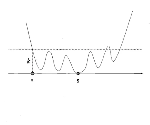
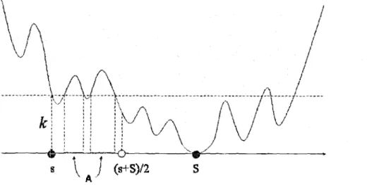
k. Hence (i) and (ii) hold.

Figure 2-2 and Figure 2-3 present examples for a typical k-convex function and a symmetric k-convex function respectively. Notice the the difference between these two functions.

Figure 2-2: An Example for k-convex Function

In the following we focus on characterizing the optimal solution for the finite horizon model. Specifically, our objective is to identify a pricing and replenishment policies that solve (2.3) or its equivalent (2.4).

It turns out that in this case the optimal policy for the a,dditive demand model is ~ignificant~ly different than the optimal policy for the general demand case. In particular, we show, in Section 2.3, that when the demand function is additive, the function

q5t is kt-concave for any

t

and hence an (s, S, p) policy is optimal. For more general demand functions, i.e., multiplicative plus additive functions, we demonstrate that

(27)

Figure 2-3: An Example for Symmetric k-convex Function

the function

4,

is not necessarily kt-concave and an (s, S, p) policy is not necessarily optimal. Indeed, in this case we show, in Section 2.4, that

dt

is symmetric k-concave which allows us to show that the optimal policy is an (s, S, A, p) policy for the general demand model. Finally, in Section 2.5, we show that our results imply that in the special case with zero fixed cost and general demand functions, a base-stock list price policy is optimal. This corollary of our results is a generalization of the resrilts in

[lo]

to general demand models.

2.3 Additive Demand

Functions

In additive demand model the demand function is assumed t,o be of the form

4

= D,(pt)

+

Pt?

(28)

Observe that a special case of this demand function is the additive linear demand jhnction in which dt = bt - atpt

+

Pt

with bt, at

>

0 for t = 1 , 2 ,

. . . ,

T .

In the following, we show, by induction, that, gt (y

,

dt (y)) is a kt-concave function of y and &(x) is a kt-concave function of x . Therefore, the optimality of an (s, S, p) policy follows directly from Lemma 2.1.

We start by proving these results under t,he assumption that the expected revenue &(d) is a strictly concave function of expected demand d. This assumption will be relaxed later in this section.

To prove that gt(y, dt(y)) is a kt-concave function of y we need the following lemma. Lemma 2 , 3 Suppose th,at gt(y, d) is jo~htly continuous in (y, d). Then, there exists a dt(y) which maximizes (2.6) such th,at y - dt(y) is a non-decreasing function of y.

We show that y - dt(y) is a non-decreasing function of y by contradiction. Assume that y'

>

y, while y' - dt (y')

<

y - dt(y). Let

d = dt(yf) - (y' - y) and d' = dt(y)

+

(y' - y).

Since dt(y)

<

d, d'

<

dt(yf), d,

d

are feasible for (2.6), and dt(y), dt(yf) are the optimal solutions of (2.6) with parameters y and y', respectively, we have that

Adding the two ineq~a~lities and using the definition of gt(y, d) in equation (2.5) with at = 1, we have

&(&(Y))

+

~t (dt (y'))

>

&(dl

+

~t (dl). (2.13) This is true since by definition y - dt(y) = y' - d' and y' - dt(y') = y - d.

Since dt(y)

<

d, d'

<

dt(yf) and d

+

d' = dt(y)

+

dt(yf), there exist

A,

p € (0, I ) , such that d = (1 - X)dt(y)

+

Xdt(y'), d' = (1 - p)dt(y)

+

pclt(yf) and X

+

p = 1. From

(29)

the concavity of ~ ~ ( d ) , we know that

The lemma thus implies that the higher the inventory level at the beginning of time period

t ,

yt, the higher the expected inventory level at the end of period

t ,

yt - d t ( y t ) . We are now ready to prove our main results for the additive demand model.

Theorem 2 . 1 (a) For any t = 1 , 2 , .

. .

, T , g t ( y , d ) is jointly continuous i n ( y , d ) and hence for any fixed y ,

Lemm,a 2.3. Furthermore,

g t ( y , d ) has

a

finite maximizer dt ( y )

= -oo for a n y d E [d,,

&]

uniformly

u h i c h satisfies

(b) For any t = 1 , 2 , . . .

,

T , g t ( y , d t ( y ) ) an,d & ( x ) are kt-concave.

(c) For a n y t = 1 , 2 , . . .

,

T ,

there exist st and St with st I St such that it is optimal t o order St

-

xt and set the selling price p t ( x t ) =

D,'

(dt

(st))

when

xt

<

s t , and n o t t o order an:yth,in,g and set pt ( x t ) = l7,l(dt(xt)) when x t 2 st.

Proof. By induction. For period 1, part ( a ) directly follows from Assumption 2.2. Parts (b) and (c) hold since g l ( y , d l ( y ) ) is concave.

Assume parts (a),(b) and (c) holds for

t

- 1. From part (c) and the continuity of

~ t - l ( ~ ,

4 ,

which implies that q52-1(x) is continuous and hence g t ( y , d ) is continuous in ( y , d ) . Thus, for any fixed y , g t ( y , d ) has a finite maximizer d t ( y ) which satisfies Lemma, 2.3.

(30)

Part (c) also implies that E{&l(y - d -

,&)I

I q5t-1(St-1) for any (y, d) and hence l i ~ n ~ ~ ~ + ~ gt(y, d) = -m for any d E

[&,

&]

uniformly by Assumption 2.2. Therefore, part (a) holds for period t .

We now focus on part (b). We show that gt (y, dt (y)) and q$(x) are kt-concave based on the a s s ~ m p t ~ i o n that (x) is kt-l-concave.

For any y

<

y', and

X

E [ O , l ] , we have by Lemma 2.3 and the assumption that

&l is kt-l-concave that

h-1((1 -

X)(Y

- @(Y) -

Pt)

+

X(Y'

- dt(yt)

-

Pt))

>

(1 - X)h-I (p -

&(Y)

- Pt)

+

A h - 1 (9' - dt

(Y')

-

Pt)

- Xkt-l.

In addition, the concavity of H?(x, d) implies that

Adding the last two inequalities and taking expectation, we get

From the definition of d t ( ( l - A) y

+

Xy'), we have

and hence,

that is, gt(y,dt(y)) is a ykt-l-concave function of y, and therefore kt-concave by Assumption 2.3 and Lemma 2.1 part (a).

We now prove that q$(x) is kt-concave in x . Since gt(y, dt(y)) is kt-concave, Lemma 2.1 part (d) implies that there exists st and St, such that St maximizes gt(y, dt(y)) and st is the smallest value of y for which gt(St, dt(St)) = gt(y, dt(y))

+

kt, and

(31)

The kt-concavity of $t can be checked directly from the kt-concavit,y of gt(y

,

d t ( y ) ) , see [5] for a proof. Hence part (b) holds for period t .

Part (c) follows directly from part (b) and Lemma 2.1.

An interesting question is whether p,(x) is a non-inmeasing function of x , as is the case for a similar model with no fixed cost (see [lo]). Unf~rt~unately, this property does not hold for our model.

Proposition 2.2 The optimal price, pt(x), is not necessarily a non-zn,creasing func-

tion of

x.

The proof is provided in Appendix A. To provide some intuition, we should point out that when the inventory level is a bit higher than the reorder point, it is not clear at all whether it would be better t o increase the selling price so as to reduce demand and hence delay the payment of the fixed ordering cost, or to decrease the selling price so as to increase demand and hence replenish inventory quickly.

2.4 General

Demand

Functions

In t,his section, we focus on the model with general demand functions (2.1). Observe that the additive demand function analyzed in the previous section is a special case of the general demand function (2.1) More importantly, multiplirative demand functions of the form dt = atDt(p) where Dt(p) = atpPbt (at

>

0, bt

>

I ) , or demand functions of the form Dt(p, et) =

Pt

+

ait(bt - atp) (at

>

0, bt

>

O), are also special cases.

Our objective in this section is two-fold. First, we demonstrate that under demand functions (2.1), &(x) rnay not be kt-concave and an (s, S. p) policy may fail to be

optimal for problem (2 4). Second, we characterize the structure of the optimal policy for the finite horizon model with general demand functions (2.1).

To characterize the optimal policy for the model with the demand functions (2.1)) one might consider using the same approach applied in Section 2.3. Unfortunately,

(32)

in this case, the function y - atdt(y) is not necessarily a non-decreasing function of y for all possible act, as is the case for additive demand functions. Hence, t,he approach employed in Section 2.3 does not work in this case.

Specifically, the next lemma, whose proof is given in Appendix B, illustrates that the function

&

(x) is in general not kt-concave.

Lemma 2 . 4 There exists an instance of problem. (2.4) with a multiplicative demand function and time independent parameters such that the functions gt(y, dt(y)) and

$t(x) are nmt kt-concave.

Of course, it is entirely possible that even if the functions gt(y, dt(y)) and $t(x) are not ,&concave for some period t , the optimal policy is still an ( s , S, p) policy. The next lemma, whose proof is given in Appendix C , shows that this is not true in general.

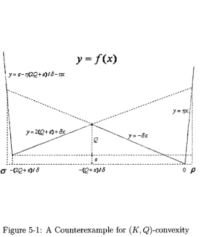
Lemma 2.5 There exists an instance of problem

(2.4)

with m~ultiplicative demand functims where an (s, S , p) policy is not optimal.

To overcome these difficulties, we apply the concept of symmetric k-convexity introduced in Section 2.2. Specifically, in the following, we show, by induction, that gt(y, dt(y)) is a sym-kt-concave function of y and q5t(x) is a sym-kt-concave f u n ~ t ~ i o n of x . Hence a characterization of the optimal pricing and ordering policies follows from Lemma 2.2.

Theorem 2.2 (a) For any t, gt(y, d) is continuous in (y, d) and hence for any fixed y, gt(yl d) has a finite maximizer dt(y) . Furthemnore,

lim gt(y,d) = -co for any d E

[dt,

dt]

unifomly .

15, '00

(b) For any t = 1,2, . . .

,

T, gt (y, dt (y)) and &(x) are sym-kt-concave.

(c) For any t = 1 , 2 ,

. . .

,

T, there exist s t and St with st

5

St and a set At C

(33)

pt = pt(St) when xt

<

s t or x E At, and not to order anything and set pt = pt(xt) otherwise.

Proof. The proof of part (a) is similar to the proof of pa.rt (a) in Theorem 2.1. We now focus on part (b).

By induction. & , ( x ) = 0 is sym-0-concave. From the ~ym-k~-~-concavity of (x), we have that for any y, y',

Also, we have that H:(y, d) is concave by Assumption 2.2. Hence, following a similar argument t o the one applied in Theorem 2.1 part (b), the function gt(y, dt(y)) is ~ym-yk~-~-concave and thus sym-kt-concave by Assumption 2.3 and Lemma 2.2 part

(4

.

From Lemma 2.2 part (d) we have

where St is the maximizer of gt (y : dt (y)) and It = {y

5

St : gt ( y

,

dt(y))

5

gt (St, dt (St)) -

kt). Furthermore, #t (x)

>

gt(x, dt(x)) for any x and +t (x)

>

-kt

+

gt(St, dt (St)) for

any x

5

St.

Let st be defined as the smallest value of y for which gt(St, dt(St)) = gt(y, dt(y))

+

kt. Note that from Lemma 2.2 part (d), (-oo, st]

c

It

and [(st

+

St)/2, oo)

c

(It)C, the complement of It.

We now prove that $t(x) is sym-kt-concave. For any x0

5

x1 and

X

E j O , l ] , let

xx = (1 - X)x0

+

Axl.

(34)

for any

x

implying that

where the second inequality holds since gt(y, dt(y)) is sym-kt-concave. Case 2: If X I E It, then

xx

5

St since

xo

5 xi

5

St and therefore

where the second inequality holds since

xI

E It and St is a global maximizer of gt(y, d t ( d ) .

Case 3: If

x1

$ I t ,

xo

E It and

xx

5

St, we have

where the second inequality holds since

xo

E It and St is a global maximizer of %(Y, d t ( ~ ) ) .

Case 4: If

xl

$ It,

xo

E It and

xx

>

St, there exists 0

5

p

5

A , such that

xx

=

(1 - p)St

+

kx17 and

where the first inequality follows from the sym-kt-concavity of gt(y, dt(y)), the third inequality from the fact that p

5

X and St maximizes gt(y, dt(y)).

(35)

Therefore, 4, (x) is sym-kt-concave.

Part (d) follows from Lemma 2.2 aad part (b) by defining A, = I,

n

[st, (st

+

W 2 1

Theorem 2.2 thus implies that the optimal policy for problem (2.3) is an (s, S, A, p) policy. Such a policy is characterized by two parameters s t and St and a set

At

C

[st, (st

+

S t ) / 2 ] , possibly empty. When the inventory level xt at the beginning of the period t is less than st or xt is in the set At, an order of size St -

xt

is made.

Otherwise, no order is placed. Thus, it is possible that an order will be placed when the inventory level

xi

E [st, (st

+

St)/2], depending on the problem instance. In any case, if an order is placed, it is always to raise the inventory level to St.

2.5 Special Case:

Zero

Fixed-Cost

Federgruen and Heching ([lo]) focused on the model with no fked ordering cost, i.e., the zero fixed cost model, both in the finite horizon and infinite horizon cases. Focusing on the finite horizon model, a key assumption in their paper implied by their Lemma 1 is that the demand function,

D t b ,

e t ) is a linear function of the price. In fact, it is not clear at all that any other demand function satisfies their main assumption, Assumption 5.

We now apply our results to the zero fixed cost case.

Corollary 2.1 Consider our model with zero fixed cost and general demand functions (2.1). I n this case, a base-stock list price policy is optimal.

Proof. By Theorem 2.2, the functions q5, a8nd gt(y, dt(y)), t = 1 , 2 , . . .

,

T , are symmetric @concave and hence, from Definition 2.3, they are concave. The ~ p t ~ i m a l i t y of t,he base-stock inventory policy directly follows from the concavity of gt(y, dt(y)) for t = 1 , 2 , . . . , T.

(36)

We now show that dt(y) is non-decreasing and therefore the optimal price pt(y) is non-increasing. If R t is strictly concave, the optimization problem maxzt2d2dt gt(g, d )

has a unique optimal solution. However, when Rt is concave, it is possible that the optimization problem has multiple optimal solutions. In the latter case, we let

which is well defined by Theorem 2.2 part (a).

Assume that there exist y

<

y' such that dt(y)

>

dt(yf). We have

Adding the t>wo inequalities and using the definition of gt(y, d) in equation (2.5), we have upon denoting r (x) = - ht (x)

+

_(x)

_,

which cannot be true since r is concave and hence has non-increasing difference. Therefore, d t ( ~ ) is non-decreasing and consequently pt(y) is non-increasing. rn

2.6 Extensions and Concluding Remarks

In this section we report on some important e~t~ensions of the finite horizon model and results.

Markovian Demand Model: The results obtained in this paper can be extended to Markovian demand models where the demand distribution a t every time period is det,ermined by an exogenous Markov chain. Specifically, our results hold under assumptions similar to those employed by Sethi and Cheng, see [25], on state dependent holding costs as well as fixed and variable ordering costs.

(37)

Markdown Model: In this case we assume that price in period

t ,

pt, is con- strained by pt

5

pt-1 for t = 2 , 3 , .

. .

,

T. In t,his case, the dynamic program (2.3) must be modified and it can be written as

<d<& - k 6 ( ~ - 2)

+

&(d) - q y

vt (x1 d') = ctx+ max,>,,rn,{& ,d ) -

+ E { - h t ( ~ - a t d -

Pt)

+

vt+i(y -

4

-

Pt,

d)). It turns out that Theorem 2.2 holds for the modified function vt (x, dl) and hence the policy introduced in Section 2.4 is optimal under the markdown set,ting. This is true since the sym-k-convexity property can be easily extended t o multi- variable functions.

2.7 Appendix A

Proof of Proposition 2.2

Proof. The following example shows that for additive demand functions, the optimal price pt(y) is not necessarily non-increasing.

Example: We conccmtrate on the last two tJime periods of problem (2.3). Since we will choose q = 0 for all

t ,

vt and pt really do not depend on

y.

Therefore, all superscripts

y

will be dropped. Let

kl = k z = 1 , ~ l = ~ 2 = 0 , h l ( ~ ) = J ~ / , d l = 4 - p , f l l = p l = l 1 hz(x) = mm{O, - 2 )

+

max{O1 x), d2 = 1 - p,

pz

= I , &

= o .

Then and 3 - / x - 31, for x >_ 2, v1(x) = otherwise

,

(

2 + ( y - l + p ) , for y - ~ + P < o , for y - l + p ~ [0,2], f 2 ( ~ 1 p ) = p ( l - ~ ) + for y - 1 + p 6 [2,3],

(

6 - ; ( ~ - 1 + ~ ) , otherwise.

(38)

Figure 2-4: A Two Periods Joint Inventory and Pricing Example

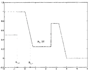
Figure 2-5: The Non-Monotonicity of the Price

Figure 2-4 depicts the f u n c h n s vl(y), vl(y) - h2(y) and f2(y,p2(y)) while Figure 2-5 presents the optimal selling price p2(y). In Figure 2-5, the dash-dotted line is p2(y)

before making the decision to order up to

S2

and solid line represents the optimal price after making the ordering decision. Notice that the subscripts T and T - 1 in

(39)

Observe that if y = 1, 9 - i + p = p ~ [ 0 , 1 ] . ~ ( l , p ) = ~ p - p ~ + 2 a n d ~ 2 ( l ) = $ , while when y = 3, y - l + p = 2 + p E [2,3], f i ( 3 , p ) z ; p - p 2 + l a n d p a ( 3 ) = i n w

2.8 Appendix

B

Proof of Lemma 2.4

Proof. Consider an instance with stationary input data for the last two periods of problem (2.3). Notice that since we will choose Q = 0 for all

t ,

$t and gt(y, d) really do not depend on y. Therefore, all superscripts y will be dropped. Also observe that in this case, vt =

&.

F o r t = 1 , 2 , let

and

a , with probability q a t =

{ -

6, with pr~ba~bility 1 - q,

where h+

>>

h-

>

0 are fixed, 6

>

1

>

a

>

0

and qa

+

(1 - q)d = 1. We will choose b

>>

h+ and a

>>

b2.

For period 1: Given h+

>>

h-

>

0 , choose b

>>

h+ and a

>>

b2. In this case, it is optimal to choose a feasible d such that y - ad is as close to

0

as possible. Therefore,

(40)

and

y / g ( b - y / a ) / a

+

h- ( y -

y/u),

for 0

5

y

5

gb, 9 1 ( Y , d l ( ~ j ) =

-qh+ ( y - cxb)

+

( 1 - q)h- ( y - lib), for gb

<

y

5

ab,

(

-h+(y - b ) , for y 2 &b

Under these assumptions, we have that

S1

= 0 , g l ( O , 0 ) = 0 and

- k , for y

5

- k / h - , v&) =

s ~ ( Y , d l ( ! / ) ) , for y

>

-k/h-

For period 2: We have that

Since b

>>

h+

>>

h-

>

0 and a

>>

b2, it is optimal to choose a feasible d such

that y -

ad

is as close to 0 as possible. Therefore, d 2 ( y ) = d l ( y ) , and

-hz(x)

+

V I ( X ) = (

Observe that g 2 ( y , d 2 ( y ) ) is decreasing for y

2

0 and directionally differentiable

for any y. For y

>

~ b , the directional differential of g 2 ( y , d 2 ( y ) ) is much larger than that for y

<

ab, since h+

>>

h-

>

0.

Denote by y = ~ k / ( h - (6 -

a ) )

=

X Q ~ ,

- / -lc

+

h-x, for x

<

- k / h - , 2h-x, for - k / h -

<

x

5

0, x / c ~ ( b - x / a ) / a

+

h - ( x - x / g ) - h+x, for 0 5 x

<

cub, -qh+(x - ~ b ) t ( 1 - q)h-(x - b b ) - h+x, for

ab

<

x

5

Qib, -2h+x

+

h+b, for

x

>

bb. \

(41)

for some X E [ O , l ] . For - y

5

y

<

~ b , we have t,hat

It remains to show that g2(y, d2(y)) is not k-concave. Observe that for y = 0, d2(y) =

0, and g2(0, 0) = 0. If g2(y,d2(y)) is k-concave, then for xo = 0, X I =

ub,

we have from the definition of k-concavity that

However, if we increase a , b and keep b2/a very small, the above inequality does not hold since X i Of, which is a c~nt~radiction. Hence g2 (y, d2 (y)) is not k-concave. Furthermore, under the above assumptions, one can see that S 2 = 0 and g2(0, 0) = 0. Therefore v2

(x)

is not k-concave, since v2 (x) = g2(x, d2 (x)) for

x

2

0. I

2.9 Appendix

C

Proof of Lemma 2.5

Proof. We extend the example of Appendix B by inve~t~igating tJime period 3. Similar to Appendix

B,

the variable cost c3 = 0. Therefore, by a similar reasoning to the one in the previous appendix, the superscripts

y

will be dropped.

Note that

-k, for y

5

-lc/(2h-), u 2 ( 4 =

g2(v, dz(y)), for y

>

-k/(2h-). For period 3: Let

(42)

and

a , with probability q

..{-

_fi,_{with pr~ba~bility}₁_-_{q ,}

We choose 6 = 2.

We choose appropriate p, E , a' and b' such that p

>>

h+

>>

a', b', and c is suffi-

ciently small. Under these assumptions, it is optimal to choose a feasible d such that y - 6 d

>

0. Therefore, we have that d

5

y l b . Using the fact that 6 = 2, one can prove that

y / b , for 0 5 y s d b ' , d3(y> =

b', f o r f i b 1 < y 5 a ( b + b ' ) by some simple ~a~lculation.

Denote by

y* = &(bl - (y

+

d)af)/2, and $ = b(b' - (27

+

c1)a')/2,

where y = q(6 - a ) h - (1/g - 1) and E' = q(fi -

a)&.

In order to simplify notation, we omit the term y/s(b - y/g)/a in g3(y, d3(y)) for

0

5

y

5

ab. This is possible, since b2

<<

a implying that y/a(b - y / ~ ) / a -+ 0+ and thus does not impact the argument below.

If fib'

<

y

<

a(b

+

b'), it is easy to check that g3(6b1, b')

2

g3(y, b').

If y

>

g ( b

+

bl), y - g b '

>

~ b . Hence we have that g3(&b1, b')

>

g3(y,d3(y)) since h+

>>

b', a', h-.

If

y / ( l -

a/&)

5

y

5

fib',

(43)

one can see from the first order optimality condition that y* maximizes g3(y, d3(y))

for y satisfying (2.15) and

For

we have that

and if

then y = 0 maximizes g3 ( y , d3(y)) for y satisfying (2.17): since gh

(c,

d3

(g))

= 0.

If

y*

satisfies (2.16) and

for some q E (0, I), then y* is the global maximizer of g3 (y . ds(y)) since p

>

h+

>>

h-.

Finally, if in addition t o (2.16), (2.18) and (2.19), we have

then we know that it is optimal t o order up t o y* when the inventory level is _-y and not tjo order when the inventory level is y = 0, since g3(0, d3(0)) = g3(0, 0 ) = 0. This implies that

Sg

<

0

<

_-y

<

s3

= y*,

and therefore, any (s,

S)

inventory policy is not optimal in this case.

The remaining task is to check whether (2.16), (2.18), (2.19) and (2.20) can hold simultaneously by choosing the appropriate parameters. Note that (2.19) is equivalent to

(44)

and the above equation, together with inequality (2.18) and the definition of y, gives that

4(1

+

q(1 - q) - q)k/y2

<

a'. (2.22)

By the definition of - y and (2.21), (2.20) is equivalent to

Now it is clear that there exists q sufficiently smadl, a', b' sufficient,l;y large compared with k , - y, h- and a', b'

<<

p, b such that (2.16)) (2.21), (2.22) and (2.23) hold.

(45)

Chapter

3 Infinite Horizon Periodic

Review

Model

In Chapter 2, we focused on the finite horizon periodic review model. In this c h a p ter, we concentrate on a corresponding infinite horizon model with stationary costs, revenue and general demand functions. We start in Sectlion 3.1 with the assumptions of the infinite horizon model. In Section 3.2 we identify properties of the best (s, S ) inventory policy for both the discounted and average profit cases. These properties, together with the concept of symmetric k-convexity, enable us t o construct solutions for the optimality equations of the discounted and average profit problems. In Section 3.4 and Section 3.5, these equations are used t o prove the optimality of a stattion- ary (s, S, p) policy for t,he infinite horizon problems with the discounted and average profit criteria, respectively. In Section 3.6 we provide some concluding remarks.

3.1 The

Model

In the infinite horizon joint inventory and pricing model the input parameters, costs, revenue and general demand functions, are assumed t,o be stationary. Thus, in what follows we drop tjhe time index subscripts from the time independent parameters. All other assumptions are similar to those of the finite horizon model in Chapter 2

(46)

Section 2.1.

For the infinite horizon joint inventory and pricing problem, both the discounted and average profit cases will be considered. In the infinite horizon expeeted discounted profit model the objective is to maximize

lim inf

V

T

y

,

T-00

for y

<

1 and any initial inventory level, where V,Y is defined in (2.2). Finally, in the infinite horizon expected average profit model the objective is to maximize

1 lim inf

-

V$

,

T+oo T

for y = 1 and any initial inventory level.

3.2 Preliminaries

Consider a stationary (s, S , p) policy defined by the reorder point s , the order-upto level S and a price p(x) which is a function of the inventory level

x.

As pointed out earlier, there is a one-to-one correspondence between price and expected demand through the mapping d = D ( p ) . Hence, from now on we use (s, S,d) and (s, S, p) interchangeably.

Given the stationary (s, S, d ) policy chosen above, let I T ( $ , x , d) be the expected y-discounted profit incurred during a horizon that starts with initial inventory level x and ends, at this period or a later period, with an inventory level no more than s. Let MY(s,

x,

d ) be the expected y-discounted time to drop from initial inventory level x t o or below s. Observe that whenever x

5

s, we have P ( s , x , d) = 0 and MY(s,

x,

d ) = 0. On the other hand when x

>

s we have

P ( s , x, d) = H Y ( x , d(x))

+

yE{IY(s,

x

- a d ( x )

-

P,

d ) ) , (3.1)

and

MY(s, x, d) = 1

+

y E { M Y ( s , x - a d ( x ) -

P,

d)). _(3.2) 46

(47)

Let

The definitions of IT ( s , x

,

d)

,

M' ( s , x

,

d ) and c? (s, S, d) imply the following p r o p erties.

Lemma 3.1 Given a n ( s , S , d ) policg,

fi) for y = 1 cT(s, S , d) is the long-run average profit;

(22) for 0

<

y

<

1 th,e function

is the infinite horizon expected discounted profit starting wwith a n initial inventory level

x.

Proof. Part (i) follows directly from t,he elementary renewal reward theory (see Ross [23]), and so does the case x

5

s for part (ii). In order to prove part (ii) for x

>

s , define r ( s ,

x,

d ) t o be the number of periods it takes t o drop the inventory level from x to or below s. Therefore, we have T ( s , x , d ) = 0 for x

5

s and

T(S,X, _d)=

1 +

T ( S , x

-

ad(x) -

P ,

d ) , for x

>

S .

The infinite horizon expected discounted profit s t a t i n g with initial inventory level x is

I Y (s, x , d)

+

E { ~ ~ ( ~ ~ ~ ~ ~ ) ) c Y ( s ,

S,

d ) / ( l - 7 ) :

which implies t,hat it suffices t,o argue that

M ~ ( S , 2 , d ) = ( 1 - ~ { y ' ( ~ ~ ~ ~ ~ ) ) ) / ( l - y ) .

(48)

which is exactly the same recursion for M r ( s , x , d) ( 3 . 2 ) . Therefore, (3.4) holds and hence part (ii) is true.

To provide intuition about (ii) observe that cY(s, S, d ) is the expected discounted profit per period for the infinite horizon expected discounted profit problem starting with an initial inventory level no more than s. Therefore, cY(s, S, d ) / ( l -

y)

is the infinite horizon expected discounted profit if we start with an initial inventory level, x , no more than s and this implies that, (ii) holds since in this case both I r i s , x , d ) and M r ( s , x , d ) are equal to zero. For x

2

s , observe that cr(s, S, d ) MY (s, x, d ) is the expected discounted profit incurred during the expected discounted time MA/(s, x , d) if we start with an init,ial inventory level no more than s . Thus, the difference between the infinite horizon expected discounted profit sta,rting with an initial inventory level no more than s and the infinite horizon expected discounted profit starting with the initial inventory level x equals

Hence (ii) follows.

We continue by assuming that the period demand is positive. Formally, this assumption says that for any realization of the ra,ndom variables 6 = ( a ,

P ) ,

a d

+

P

2

a d -

+

,O

>

77

>

0 for some q and any d E

[d,

21.

This assumption will be relaxed by perturbing a and analyzing the limiting behavior of the best (s, S ) inventory policy.

For any given (s, S)

,

let cY(s, S) be the optimal value of problem max c Y ( s , S , d ) .

d:&d(x)>_d

Define

where

gY(x,s,S,s',d) = HY(x,d) -cY(s,S)+yE{$'(x - a d - P , s , S , s t ) ) . 48

(49)

Let $Y(x, S , S) = $Y(x, s , S, s). For any feasible expected demand function d , let g7(x, s , S, d) = I Y ( s , x, d) - C ~ ( S , S ) M Y ( s , x , d ) . _(3.7) Then from the recursions for 1 7 (3.1) and MY (3.2)) we have that

0, for

x

5

s, gY(x, S , S, d ) =

H ' ( x , d(x)) - cr(s, S)

+

yE{$Y(x - a d ( x ) -

P ,

s, S, d)), for x

>

s.

Lemma 3.2 For any x,

lim sup $' (x, S , S, d ) = $Y (x: S, S). d : &d(x)>d

In particular, $'(S, s , S ) = k .

Proof. We argue by induction that $Y(x, s , S, d )

5

+Y(x, s , S ) for any feasible function d and any x. It is clearly true for x

5

s since in this case both functions equal zero. Assume that it is t,rue for any x with x

5

y for some y. ?Ve prove that it is also true for x

<

y

+

v.

In fact, for x

>

s ,

$YE,

S, S, d ) = HY(x, d(x)) - cY(s, S)

+

YE{$~(X

- a d ( x ) -

P ,

S: S, d ) )

<

HY(x, d(x)) - cY(s, S)

+

yE{$T(x - d ( x ) -

P,

S , S)) -

5

~ ~ X ~ ~ ~ > ~ H ~ ( X , ~ ) - C ' ( S , S ) + -- f i / E { ~ Y ( x - ~ d - P , ~ , S ) )

= $ Y ( x , s , s ) :

where the first inequality is justified by the inductlion assumption. On the other hand, for any given E

>

0, choose a function d, such that for any x

>

s

We have that $Y(x, S, S, dE) converges to $Y(x, S , S) uniformly over any bounded set

as E J 0. Thus for any x,

limsup $ ~ ~ ( x , s , S , d ) = $ Y ( ~ , ~ ~ , S ) d: & d ( x ) 2 4

Coordinating inventory control and pricing strategies