HAL Id: inserm-03211914
https://www.hal.inserm.fr/inserm-03211914
Submitted on 29 Apr 2021
HAL is a multi-disciplinary open access
archive for the deposit and dissemination of
sci-entific research documents, whether they are
pub-lished or not. The documents may come from
teaching and research institutions in France or
abroad, or from public or private research centers.
L’archive ouverte pluridisciplinaire HAL, est
destinée au dépôt et à la diffusion de documents
scientifiques de niveau recherche, publiés ou non,
émanant des établissements d’enseignement et de
recherche français ou étrangers, des laboratoires
publics ou privés.
Performance of approaches relying on multidimensional
intermediary data to decipher causal relationships
between the exposome and health: A simulation study
under various causal structures
Solène Cadiou, Xavier Basagaña, Juan Gonzalez, Johanna Lepeule, Martine
Vrijheid, Valérie Siroux, Rémy Slama
To cite this version:
Solène Cadiou, Xavier Basagaña, Juan Gonzalez, Johanna Lepeule, Martine Vrijheid, et al..
Perfor-mance of approaches relying on multidimensional intermediary data to decipher causal relationships
between the exposome and health: A simulation study under various causal structures. Environment
International, Elsevier, 2021, 153, pp.106509. �10.1016/j.envint.2021.106509�. �inserm-03211914�
Environment International 153 (2021) 106509
Available online 25 March 2021
0160-4120/© 2021 The Authors. Published by Elsevier Ltd. This is an open access article under the CC BY-NC-ND license
(http://creativecommons.org/licenses/by-nc-nd/4.0/).
Performance of approaches relying on multidimensional intermediary data
to decipher causal relationships between the exposome and health: A
simulation study under various causal structures
Sol`ene Cadiou
a, Xavier Basaga˜na
b,c,d, Juan R. Gonzalez
b,c,d, Johanna Lepeule
a,
Martine Vrijheid
b,c,d, Val´erie Siroux
a, R´emy Slama
a,*aTeam of Environmental Epidemiology, IAB, Institute for Advanced Biosciences, Inserm, CNRS, CHU-Grenoble-Alpes, University Grenoble-Alpes, Grenoble, France bISGlobal, Barcelona Institute for Global Health, Barcelona, Spain
cUniversitat Pompeu Fabra (UPF), Barcelona, Spain dCIBER Epidemiología y Salud Pública (CIBERESP), Spain
A R T I C L E I N F O
Handling Editor: Shoji F. Nakayama
Keywords: Exposome Variable selection Multilayer Omics Specificity Sensitivity Reverse causality A B S T R A C T
Challenges in the assessment of the health effects of the exposome, defined as encompassing all environmental exposures from the prenatal period onwards, include a possibly high rate of false positive signals. It might be overcome using data dimension reduction techniques. Data from the biological layers lying between the expo-some and its possible health consequences, such as the methylome, may help reducing expoexpo-some dimension. We aimed to quantify the performances of approaches relying on the incorporation of an intermediary biological layer to relate the exposome and health, and compare them with agnostic approaches ignoring the intermediary layer. We performed a Monte-Carlo simulation, in which we generated realistic exposome and intermediary layer data by sampling with replacement real data from the Helix exposome project. We generated a Gaussian outcome assuming linear relationships between the three data layers, in 2381 scenarios under five different causal structures, including mediation and reverse causality. We tested 3 agnostic methods considering only the exposome and the health outcome: ExWAS (for Exposome-Wide Association study), DSA, LASSO; and 3 methods relying on an intermediary layer: two implementations of our new oriented Meet-in-the-Middle (oMITM) design, using ExWAS and DSA, and a mediation analysis using ExWAS. Methods’ performances were assessed through their sensitivity and FDP (False-Discovery Proportion). The oMITM-based methods generally had lower FDP than the other approaches, possibly at a cost in terms of sensitivity; FDP was in particular lower under a structure of reverse causality and in some mediation scenarios. The oMITM–DSA implementation showed better perfor-mances than oMITM–ExWAS, especially in terms of FDP. Among the agnostic approaches, DSA showed the highest performance. Integrating information from intermediary biological layers can help lowering FDP in studies of the exposome health effects; in particular, oMITM seems less sensitive to reverse causality than agnostic exposome-health association studies.
1. Introduction
The exposome concept acknowledges that individuals are exposed simultaneously to a multitude of environmental factors from concep-tions onwards (Wild, 2005). The exposome, understood as the totality of the individual environmental (i.e. non-genetic exogenous) factors, may
explain an important part of the variability in chronic diseases risk (Manrai et al., 2017; Sandin et al., 2014; Visscher et al., 2012). During the last decade, environmental epidemiology started embracing the exposome concept (Haddad et al., 2019) (see e.g. (Agier et al., 2019; Lenters et al., 2016; Patel et al., 2010)). Such studies typically face an issue encountered in many fields (Runge et al., 2019), that of efficiently
Abbreviations: BMI, Body-Mass-Index; DAG, Directed Acyclic Graph; DSA, Deletion-Substitution-Addition algorithm; ExWAS, Exposome-Wide Association Study;
FDP, False-Discovery Proportion; LASSO, Least Absolute Shrinkage and Selection Operator; MITM, Meet-in-the-Middle; oMITM, oriented Meet-in-the-Middle. * Corresponding author at: Team of environmental epidemiology, IAB, Institute for Advanced Biosciences, Inserm, CNRS, CHU-Grenoble-Alpes, University Grenoble-Alpes, All´ee de Alpes, Grenoble, France.
E-mail address: Remy.slama@univ-grenoble-alpes.fr (R. Slama).
Contents lists available at ScienceDirect
Environment International
journal homepage: www.elsevier.com/locate/envint
https://doi.org/10.1016/j.envint.2021.106509
identifying the causal predictors of an outcome among a set of possibly correlated variables of intermediate to high dimension (currently, a few hundred to a few thousand variables). The correlation within the exposome (Tamayo-Uria et al., 2019) was shown to entail a possibly high rate of false positive findings, in particular when using ExWAS (exposome-wide association study), i.e. parallel univariate models with correction for multiple testing (Agier et al., 2016). Recent studies, typically conducted among a few hundred or thousand subjects, are also expected to have limited power (Chung et al., 2019; Siroux et al., 2016; Slama and Vrijheid, 2015; Vermeulen et al., 2020). In addition, they can suffer from reverse causality: if exposures are measured by biomarkers at the same time as the outcome, this opens the possibility of the health outcome influencing some components of the exposome. For example, the serum concentration of persistent compounds can be influenced by the amount of body fat, which is related to health outcomes such as obesity or cardiovascular disorders (Cadiou et al., 2020). The potential for reverse causality is even stronger if biomarkers of effect (e.g. bio-markers of oxidative stress or inflammation) are considered to be part of the exposome, as sometimes advocated (Rappaport, 2012; Vermeulen et al., 2020). Indeed, these may also be consequences of the considered health outcome.
Benchmark studies and reviews tried to identify which statistical methods could help to face some of these issues (Agier et al., 2016; Barrera-G´omez et al., 2017; Lazarevic et al., 2019; Lenters et al., 2018). Dimension reduction tools are a relevant option to consider (Chadeau- Hyam et al., 2013). Dimension reduction can be achieved by purely statistical approaches, or rely on external (e.g., biological) information. Past simulation studies focused on statistical dimension reduction techniques and generally assumed a simple causal structure and that the variability of the outcome explained by the exposome was higher than 5% (Agier et al., 2016; Barrera-G´omez et al., 2017; Lenters et al., 2018): within this framework, they showed that dimension reduction tech-niques such as regression-based variable selection methods simulta-neously considering multiple variables were more efficient than the ExWAS to control the false positive rate (Agier et al., 2016). When it comes to non-purely statistical dimension reduction approaches, it may be relevant to try relying on biological parameters, including ‘omic (methylome, transcriptome, metabolome…), inflammatory or immu-nologic markers, possibly acting as intermediary factors between the exposome and health. This logic is embodied in the Meet-in-the-Middle (MITM) design (Chadeau-Hyam et al., 2011; Jeong et al., 2018), which detects “intermediary” biomarkers associated with both exposures and the health outcome. To relate the exposome to child body mass index (BMI), we recently applied a tailored MITM design (Cadiou et al., 2020), named hereafter “oriented Meet-in-the-Middle” (oMITM), with a dimension reduction aim, and using methylation data to reduce expo-some dimension. The oMITM approach used here and in (Cadiou et al., 2020) shares with the classical MITM the principle of separated steps testing the association within the three layers. However, in our oMITM design, the steps followed a specific order and we added an adjustment on the outcome at the step testing the association between the exposures and the methylome. Moreover, the objectives differ as our aim is not to identify relevant biomarkers as done in the first studies using MITM (Huang et al., 2018; Jeong et al., 2018; Vineis et al., 2020, 2013) but to use the methylome to reduce the exposome dimension in order to point more accurately the exposures possibly influencing the outcome.
From our previous work (Cadiou et al., 2020), we hypothesize that oMITM 1) could allow lowering the high FDP reported for agnostic ExWAS, and 2) could be less sensitive to reverse causality than agnostic dimension reduction methods. This might be obtained at a cost of a decreased sensitivity, in particular as the proportion of exposures whose health effect is not mediated by the considered layer increases (Cadiou et al., 2020). Specifically, we aimed here to test if methods relying on intermediary multidimensional biological data allow to more efficiently identify the causal predictors of a health outcome among a large number of environmental factors. We both considered methods making use of
information on potential mediators of the health effects of exposures and agnostic methods ignoring the intermediate layer, and compared their sensitivity and False Discovery Proportion (FDP). Data were generated assuming five different possible causal models, including reverse cau-sality, for realistically low values of the share of the outcome variability explained by the exposome. After comparing the methods using simu-lated data, in a second section, we use causal inference theory to discuss which designs may be most adapted under each possible causal structure.
2. Materials and methods
2.1. Overview of the simulation
We relied on a Monte-Carlo simulation to compare the efficiency of methods aiming at identifying which components of the exposome influenced a health outcome under various causal models and hypoth-eses (altogether defining a total of 2381 scenarios). Exposome, inter-mediary layer and outcome data were generated under these various scenarios. For each scenario, 100 datasets were simulated (see below). The 6 methods compared, as well as two control methods (see below), were applied to each dataset and their performances were assessed, and synthesized over all datasets related to a given scenario.
2.2. Causal structures considered
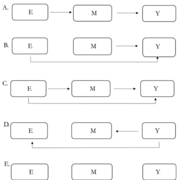
Five different causal structures were considered (see Fig. 1): in structures A, B and C the exposome (E) affected the outcome (Y) directly or/and indirectly. In A, there was no direct effect from E to Y, all the effect being mediated by the intermediary layer (i.e. an “indirect effect” in the mediation analysis terminology (Vanderweele and Vansteelandt, 2009)). B assumed a causal link from M to Y and a direct effect from E to Y, without mediation through M. C assumed both a direct and an indi-rect effect of E on Y. Structure D is a situation with reverse causal links from Y to M and from Y to E. Structure E assumed total independence between the three layers.
Fig. 1. Causal structures considered in the simulation study of the performance
of methods relating a layer of predictors E (e.g., the exposome) to a health outcome or parameter Y using a layer of possibly intermediary parameters M (e. g. biological parameters such as DNA methylation).
Environment International 153 (2021) 106509
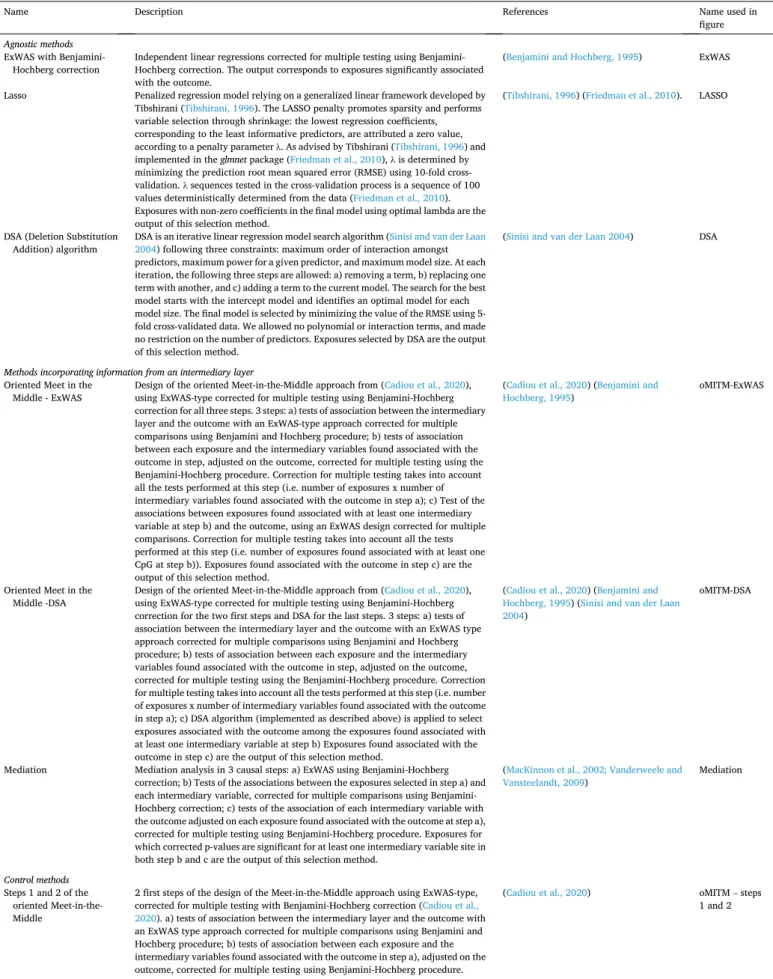
Table 1
Details of the methods compared in the simulation study.
Name Description References Name used in
figure
Agnostic methods
ExWAS with Benjamini-
Hochberg correction Independent linear regressions corrected for multiple testing using Benjamini- Hochberg correction. The output corresponds to exposures significantly associated with the outcome.
(Benjamini and Hochberg, 1995) ExWAS
Lasso Penalized regression model relying on a generalized linear framework developed by Tibshirani (Tibshirani, 1996). The LASSO penalty promotes sparsity and performs variable selection through shrinkage: the lowest regression coefficients, corresponding to the least informative predictors, are attributed a zero value, according to a penalty parameter λ. As advised by Tibshirani (Tibshirani, 1996) and implemented in the glmnet package (Friedman et al., 2010), λ is determined by minimizing the prediction root mean squared error (RMSE) using 10-fold cross- validation. λ sequences tested in the cross-validation process is a sequence of 100 values deterministically determined from the data (Friedman et al., 2010). Exposures with non-zero coefficients in the final model using optimal lambda are the output of this selection method.
(Tibshirani, 1996) (Friedman et al., 2010). LASSO
DSA (Deletion Substitution
Addition) algorithm DSA is an iterative linear regression model search algorithm (2004) following three constraints: maximum order of interaction amongst Sinisi and van der Laan predictors, maximum power for a given predictor, and maximum model size. At each iteration, the following three steps are allowed: a) removing a term, b) replacing one term with another, and c) adding a term to the current model. The search for the best model starts with the intercept model and identifies an optimal model for each model size. The final model is selected by minimizing the value of the RMSE using 5- fold cross-validated data. We allowed no polynomial or interaction terms, and made no restriction on the number of predictors. Exposures selected by DSA are the output of this selection method.
(Sinisi and van der Laan 2004) DSA
Methods incorporating information from an intermediary layer
Oriented Meet in the
Middle - ExWAS Design of the oriented Meet-in-the-Middle approach from (using ExWAS-type corrected for multiple testing using Benjamini-Hochberg Cadiou et al., 2020), correction for all three steps. 3 steps: a) tests of association between the intermediary layer and the outcome with an ExWAS-type approach corrected for multiple comparisons using Benjamini and Hochberg procedure; b) tests of association between each exposure and the intermediary variables found associated with the outcome in step, adjusted on the outcome, corrected for multiple testing using the Benjamini-Hochberg procedure. Correction for multiple testing takes into account all the tests performed at this step (i.e. number of exposures x number of intermediary variables found associated with the outcome in step a); c) Test of the associations between exposures found associated with at least one intermediary variable at step b) and the outcome, using an ExWAS design corrected for multiple comparisons. Correction for multiple testing takes into account all the tests performed at this step (i.e. number of exposures found associated with at least one CpG at step b)). Exposures found associated with the outcome in step c) are the output of this selection method.
(Cadiou et al., 2020) (Benjamini and
Hochberg, 1995) oMITM-ExWAS
Oriented Meet in the
Middle -DSA Design of the oriented Meet-in-the-Middle approach from (using ExWAS-type corrected for multiple testing using Benjamini-Hochberg Cadiou et al., 2020), correction for the two first steps and DSA for the last steps. 3 steps: a) tests of association between the intermediary layer and the outcome with an ExWAS type approach corrected for multiple comparisons using Benjamini and Hochberg procedure; b) tests of association between each exposure and the intermediary variables found associated with the outcome in step, adjusted on the outcome, corrected for multiple testing using the Benjamini-Hochberg procedure. Correction for multiple testing takes into account all the tests performed at this step (i.e. number of exposures x number of intermediary variables found associated with the outcome in step a); c) DSA algorithm (implemented as described above) is applied to select exposures associated with the outcome among the exposures found associated with at least one intermediary variable at step b) Exposures found associated with the outcome in step c) are the output of this selection method.
(Cadiou et al., 2020) (Benjamini and Hochberg, 1995) (Sinisi and van der Laan 2004)
oMITM-DSA
Mediation Mediation analysis in 3 causal steps: a) ExWAS using Benjamini-Hochberg correction; b) Tests of the associations between the exposures selected in step a) and each intermediary variable, corrected for multiple comparisons using Benjamini- Hochberg correction; c) tests of the association of each intermediary variable with the outcome adjusted on each exposure found associated with the outcome at step a), corrected for multiple testing using Benjamini-Hochberg procedure. Exposures for which corrected p-values are significant for at least one intermediary variable site in both step b and c are the output of this selection method.
(MacKinnon et al., 2002; Vanderweele and
Vansteelandt, 2009) Mediation
Control methods
Steps 1 and 2 of the oriented Meet-in-the- Middle
2 first steps of the design of the Meet-in-the-Middle approach using ExWAS-type, corrected for multiple testing with Benjamini-Hochberg correction (Cadiou et al., 2020). a) tests of association between the intermediary layer and the outcome with an ExWAS type approach corrected for multiple comparisons using Benjamini and Hochberg procedure; b) tests of association between each exposure and the intermediary variables found associated with the outcome in step a), adjusted on the outcome, corrected for multiple testing using Benjamini-Hochberg procedure.
(Cadiou et al., 2020) oMITM – steps
1 and 2
(continued on next page)
2.3. Generation of realistic exposome, intermediary layer and outcome data
To build datasets according to these causal structures, we first generated independent variables corresponding to a set of exposures (our exposome) and a biological layer (e.g., corresponding to metab-olomic signals or methylation levels at various sites on the DNA) by independently sampling with replacement real data of the exposome and DNA methylome from 1173 individuals of HELIX project (Cadiou et al., 2020; Maitre et al., 2018; Vrijheid et al., 2014). For the exposome, 173 quantitative variables corresponding to the exposures were obtained from the real prenatal and postnatal child exposome data of Helix, selecting only the quantitative exposures and covariates. Variables were then standardized and bounded (a standardized value greater than 3 in absolute value being replaced by a value lower than 3 in absolute value randomly drawn in the distribution). For the intermediary layer, 2284 quantitative variables were obtained from the real methylome data of Helix and the a priori selection of CpGs related to BMI via a genetic database performed in Cadiou et al. (2020) by selecting only enhancers CpGs belonging to selected pathways. These variables were standardized.
From this sampled dataset, in which the exposure E and the meth-ylome M were, by construction, independent, we used linear models to possibly add an hypothesized effect of some exposures on variables of the intermediate layer, and to generate a health outcome possibly related to E and/or M according to the above-mentioned causal struc-tures (Fig. 1): in causal structures A, B and C, assuming a causal effect of the exposome or the intermediate layer on the outcome, the outcome (Y) was drawn from a normal distribution to which potential effects of E and M were added. The variance of this distribution was set to ensure that the total variability explained by E and M was that defined by the desired scenario. To simulate a reverse causal link (structure D, Fig. 1) and a situation without causal link between the three layers (structure E), we generated the outcome by bootstrapping the real child BMI data of HELIX cohorts; a linear effect of the outcome was added to the exposome and to the methylome for causal structure D (all scripts are available in Supplementary Material 2). BMI was standardized accord-ing to WHO guidelines (Cadiou et al., 2020; de Onis et al., 2007).
For each causal structure, different scenarios varying the intensity of the hypothesized associations and the number of predictors from each layer were generated: in particular, for the structures displaying an ef-fect of E on Y, the total variability of Y explained by E and M, fixed within a scenario, varied between 0.01 and 0.4 and the number of true predictors of Y within E varied between 1 and 25; the number of ele-ments of M with an effect on Y varied between 10 and 100 in the causal structures assuming such an effect. The parameters of the different scenarios are detailed in Supplementary Table 1. For each scenario considered, 100 datasets were simulated.
The simulation (detailed in Supplementary Material 1) additionally made the following assumptions:
•All direct effects of a variable on another were assumed to be linear.
• The magnitude (i.e., slope) of all effects from the predictor variables of a given layer (e.g. E) on the predicted variables of another layer were identical within a given scenario.
• A variable from M could not be affected by more than one exposure. In consequence, when multiple exposures were assumed to affect the intermediary layer, the number of variables from M affected by E was a multiple of the number of exposures.
2.4. Methods to relate the exposome and health
For each generated dataset, we applied 8 different statistical methods, detailed in Table 1:
– three “agnostic” methods ignoring the intermediary layer: ExWAS with Benjamini-Hochberg correction (Benjamini and Hochberg, 1995), Lasso (Friedman et al., 2019; Tibshirani, 1996), Deletion Substitution Addition (DSA) algorithm (Sinisi and van der Laan, 2004);
– three methods using the intermediary layer to reduce the dimension of the exposome: two implementations of our oMITM-design (Cadiou et al., 2020) and a mediation analysis using parallel simple linear regressions (Küpers et al., 2015; MacKinnon et al., 2002); – two “control” methods: “ExWAS steps 1 and 2” and “ExWAS on
subsample”, meant to inform the comparison between the results of the previous methods (see below and Table 1), and not to provide directly interpretable results.
The oMITM design, detailed in Table 1 and implemented by Cadiou et al. (2020), consists in three series of association tests: a) between the intermediary layer M and the outcome Y, allowing to identify compo-nents of M associated with Y; b) between the compocompo-nents of the inter-mediary layer selected at step a) and the exposures E, with an adjustment on the outcome Y; c) between the exposures selected at step b) and the outcome Y (see (Cadiou et al., 2020) for details). Various statistical methods can be used at steps a), b) and c). We tested two different implementations of the oMITM design: the first one (oMITM- ExWAS) used ExWAS-type methods at all steps, i.e. a series of parallel linear regression models (one per tested predictor) corrected for multi-ple testing using Benjamini-Hochberg procedure (Benjamini and Hoch-berg, 1995); the second oMITM implementation used an ExWAS-type approach at steps a) and b) and DSA algorithm at step c). DSA (Sinisi and van der Laan, 2004) is is an iterative linear regression model search algorithm, which has been shown to provide the best performance (assessed as the compromise between sensitivity and FDP) in studies relating the exposome to health, compared to other common methods including ExWAS (Agier et al., 2016). DSA was not considered for steps a) and b) as, as a wrapper method, it is not computationally feasible to use it on a set of covariates of dimension higher than a few hundred. 2.5. Assessing methods’ performances
To assess the characteristics of each scenario, variabilities of Y explained by the true predictors of the exposome, by the true predictors of M and by both were measured and their mean and standard deviation
Table 1 (continued)
Name Description References Name used in
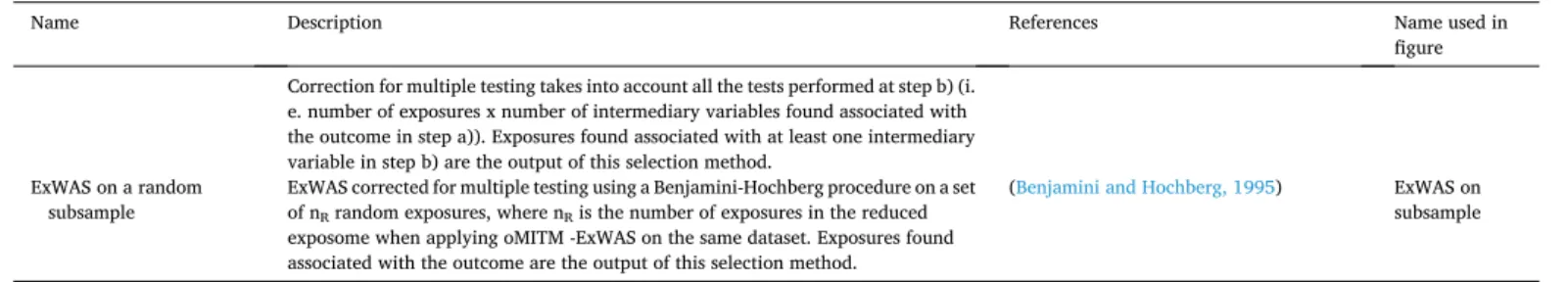
figure Correction for multiple testing takes into account all the tests performed at step b) (i.
e. number of exposures x number of intermediary variables found associated with the outcome in step a)). Exposures found associated with at least one intermediary variable in step b) are the output of this selection method.
ExWAS on a random
subsample ExWAS corrected for multiple testing using a Benjamini-Hochberg procedure on a set of nR random exposures, where nR is the number of exposures in the reduced
exposome when applying oMITM -ExWAS on the same dataset. Exposures found associated with the outcome are the output of this selection method.
(Benjamini and Hochberg, 1995) ExWAS on
Environment International 153 (2021) 106509 were computed over the 100 runs. For causal structures A and C, the
variability explained by the exposome for each variable of M affected by the exposome was also measured and averaged. Then the mean and standard deviation of this averaged variability were computed over the 100 runs. For causal structures D and E, the variability explained by Y was measured for each variable of M or each exposure predicted and means and standard deviations were computed across the exposome and the intermediary layer.
To compare methods, for each scenario of causal structures A, B and C, false discovery proportion (FDP) and sensitivity to identify true pre-dictors within the exposome were measured and mean and standard deviation were computed. FDP was defined as the proportion of expo-sures that were not causal predictors among the expoexpo-sures selected. When no exposure was selected, FDP was set to 0. Sensitivity was defined as the proportion of exposures selected among the true causal predictors. For scenario from structures D and E, for which there were no true predictors of Y, the mean and standard deviations of the number of predictors found were computed over the 100 runs. The “sensitivity” to detect exposures affected by Y was also computed. In causal structures A, B and C, methods’ performances were compared in term of FDP, sensitivity and accuracy (defined as the sum of sensitivity and 1 – FDP). The script, developed in R, is provided in Supplementary Material 2. 2.6. Comparisons between oMITM, mediation and direct association test using structural causal modelling theory
We used the theory of structural causal modelling (Pearl, 2009, 1995) to identify in which causal structures a causal association could be expected to be identified using the oriented Meet-in-the-Middle design in the simpler situation of three unidimensional variables (e.g. one exposure, one CpG, one outcome, ignoring the higher dimension of E and M in our simulation). Twenty-five Directed Acyclic Graphs (DAG) were assessed, corresponding to the 27 theoretical possibilities combining 3 variables with 3 modalities (no causal link, causal link, reverse causal link) without the two diagrams corresponding to cyclic graphs (E → M → Y → E and Y → M → E → Y). For each causal structure, potential bias were identified for each association test through the ex-istence of a spurious association between two variables because of a backdoor path not controlled for or because of adjustment for a collider (Pearl, 2009, 1995). This allowed to determine if oMITM would be able to show an association, assuming that statistical power was sufficient. We determined for each causal structure if the design was expected to provide a false-positive, false-negative, true-positive or true negative finding, according to the theoretical output (exposure selected or not) and the presence of a causal link from the exposure to the outcome in the causal structure considered. Similar analyses were done for the media-tion design (see Table 1), for a design similar to the oMITM but without adjustment on the outcome in the second step b) (which corresponds to the MITM design most commonly implemented in the literature ( Cha-deau-Hyam et al., 2011)), and for the basic association test between E and Y ignoring M.
3. Results
3.1. Performances under causal structures assuming an effect of the exposome on health
The characteristics of the scenarios under causal structures assuming an effect of the exposome on health (structures A, B and C) are sum-marized in Supplementary Table 2. On average over these three struc-tures, DSA and oMITM-DSA provided the highest accuracy; FDP was lower for oMITM-DSA and sensitivity higher for DSA (Table 2).
When we considered the three causal structures A, B and C sepa-rately, the most accurate method differed between causal structures. When we assumed that the totality of the effect of E on Y was mediated by M (structure A), the variability of Y explained by E was necessarily
lower than under the other causal structures with direct E-Y relation (Supplementary Table 2). The method maximizing accuracy was oMITM-DSA (Table 2). It was immediately followed by the oMITM- ExWAS and then the mediation analysis. Average sensitivity was higher than 0.095 for all the agnostic and non-agnostic methods and it increased with the variability of E explained by Y. The method dis-playing the lowest FDP was oMITM-DSA (average FDP across scenarios, 0.038), which also showed one of the lowest sensitivities on average (0.095); however, as soon as the variability explained by the exposome was above 0.1, its sensitivity was above 0.70 while its FDP remained below 0.20 (Fig. 2). In a few scenarios (when the variability explained by the exposome was between 0.05 and 0.1, see Fig. 2 and Supplementary Fig. 1), oMITM-DSA even showed a better sensitivity than its agnostic counterpart, DSA, with a similar FDP. When the variability explained by the exposome was low (below 0.01), oMITM-DSA often did not select any predictor, contrarily to DSA, which always showed an average non- null FDP in this range of variabilities. oMITM-ExWAS and mediation had an average FDP and an average sensitivity that were both of 0.1. Overall, the reduced exposome selected by the two oMITM designs (after steps 1 and 2 of oMITM) contained more true predictors than a random set of exposures of the same dimension; this can be seen by comparing the sensitivity of oMITM-ExWAS to the sensitivity of the control method ExWAS on subsample (Fig. 3A), which was lower in all scenarios. Inter-estingly, the FDP of oMITM-ExWAS and ExWAS on subsample were similar and lower than the FDP of ExWAS. This shows the influence of the dimension on the FDP for ExWAS-based methods and illustrates the benefit of the dimension reduction steps provided by oMITM.
Coming to the agnostic methods, DSA and ExWAS displayed similar global performances (Table 2), but DSA showed better (lower) FDP in the few scenarios for which the variability explained by E was higher than 0.1 (Fig. 2A and B). LASSO displayed the highest FDP (average, 0.41) and had a high FDP even when the variability explained by the predictors was low (Fig. 2A), as, contrarily to the other methods, it most often selected a non-null number of variables in these situations ( Sup-plementary Fig. 1C).
When we assumed that the exposome directly influenced health (without mediation by the intermediate layer, structure B), all methods relying on information from the intermediary layer unsurprisingly showed very low sensitivity (lower than 0.010); they also had very low FDP (lower than 0.013, Table 2), as they did not select any exposure in most scenarios (see Supplementary Fig. 2C). Coming to the agnostic methods, their sensitivity increased with the variability of Y explained by E (Fig. 4B). Among both types of methods, the one maximizing ac-curacy was DSA, which performed far better than the other methods (Table 2). oMITM-DSA ranked second in terms of accuracy: there were some scenarios (when both variabilities explained by E and M were higher than 0.1) in which oMITM methods selected some exposures that were true predictors (Fig. 4B and Supplementary Fig. 2A). In these scenarios, oMITM-DSA showed good sensitivity (average, 50%) and very good FDP (lower than 15%). Indeed, counter-intuitively, for these sce-narios, the reduced exposome selected by oMITM design was non-empty and contained more true predictors than would be selected by chance (this can be seen in Fig. 3B by comparing the sensitivity of oMITM- ExWAS to the sensitivity of ExWAS on subsample, which was always lower). On the contrary, mediation provided a null sensitivity, always failing to detect true predictors (Fig. 4B). This relatively good behavior of oMITM under causal structure B can be explained by the selection bias (Hern´an et al., 2004) induced in step b) of the oMITM design when adjusting on Y: a “spurious” link between E and Y is created, leading to add some causal predictors of Y in the reduced exposome.
For structure C, the situation with both direct and indirect effects of the exposome on health, performances ranged between those observed in scenarios A and B; oMITM-DSA and DSA were, again, the methods with the highest accuracy (Fig. 5).
3.2. Performance under causal structures without effect of the exposome In a situation with causal links from Y to E and to M (corresponding to reverse causality, structure D, scenarios described in Supplementary Table 3), all agnostic methods displayed a non-null number of hits, with the number of hits increasing when the variability of E explained by Y increased (Fig. 6B and Supplementary Fig. 4A). This is consistent with the fact that these methods cannot distinguish an influence of E on Y from an influence of Y on E: as shown in Fig. 6, as the variability of exposures explained by Y increased, exposures were more often selected as hits. This proportion of hits had values similar to the sensitivity dis-played by these agnostic methods in structures A, B and C.
Both oMITM methods selected no exposure most of the time (Fig. 6
and Table 2). On the contrary, the mediation analysis showed a non-null number of hits as soon as the mean variability of E explained by Y was higher than 0.05 and the mean variability of M explained by Y was higher than 0.3: the number of exposures influenced by Y selected by mediation analysis increased with the share of the variability of M explained by Y (see Fig. 6A).
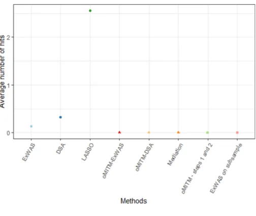
The situation without any causal link (structure E) can be seen as the limit of all four precedent structures when the strength of all associa-tions approaches zero. All methods using methylome information selected no exposure, while agnostic methods erroneously selected some exposures, with LASSO showing the highest error rate (Table 2 and
Fig. 7).
3.3. Comparisons between methods using causal inference theory Applying causal inference theory, we compared the number of possible causal structures under which various analytical strategies would be able to identify a true effect of an exposure on health in ideal situations of large sample size. The results are synthesized in Table 3, while details of results for each causal situation are displayed in Sup-plementary Table 4. In Supplementary Table 5, the step-by-step results for oMITM are detailed.
A test of association between E and Y ignoring M was expected to properly identify all situations in which E influenced Y (0 false negative, 9 true positive results, Table 3), but also identified associations corre-sponding to reverse causality (10 false positive results). Among the methods using the intermediary variable M, oMITM and MITM without adjustment on Y both displayed false negative results under 2 causal structures (structures J and K, Supplementary Table 4). The mediation test displayed false negative results under 2 additional causal structures (Table 3): in particular, contrarily to oMITM, it was not able to detect the structure A in which E affects Y indirectly through M (structure A,
Supplementary Table 4, Fig. 1). Coming to false positives, oMITM was the design minimizing the false positive findings (6 versus at least 8 for any other design). MITM led to false positives in two situations of reverse causality to which oMITM, on the contrary, was not sensitive (structures D and Q, Supplementary Table 4). The mediation method displayed, similarly to MITM, 8 false positives.
Overall, oMITM was the design giving true results (true positive or true negative) in the highest number of causal structures (17 structures, versus 15 for tests of association ignoring M and for MITM not adjusted for Y, and 13 for mediation analysis, Table 3).
4. Discussion
We implemented a simulation considering five different causal structures to identify in which contexts specific methods making use of information from an intermediary biological layer could be more effi-cient than specific agnostic algorithms to identify components of the exposome influencing health. Our simulation study demonstrated that the oMITM design has high accuracy under various causal structures. In particular, it allows to avoid false-positive associations in some struc-tures corresponding to reverse causality more efficiently than all other
tested designs which detected spurious associations, in particular those not making use of the intermediary layer. Moreover, in the causal structures with a direct effect of the exposome on the outcome, for which other methods sometimes suffer from an high false positive rate, oMITM allows decreasing false positive rate while conserving a good sensitivity. 4.1. Strengths and limitations
Former simulations about the performance of statistical methods to assess exposome-health associations generally considered simpler causal structures, without any intermediate layer nor reverse causality (Agier et al., 2016; Barrera-G´omez et al., 2017; Lenters et al., 2018). Other simulations considered multi-layered data, but often with an aim distinct from ours, such as the quantification of the share of the effect of an exposure on an outcome mediated by a high dimension intermediate layer (Barfield et al., 2017; Tobi et al., 2018). Similarly to previous simulations Agier et al., 2016; Barrera-G´omez et al., 2017; Lenters et al., 2018), we made the assumptions of lack of confounding and measure-ment error. We did consider only continuous variables in all the three layers and further simulations would be necessary to generalize our results for example to non-continuous outcomes.
We only studied experimentally 5 of the 25 possible causal structures theoretically possible, deferring the discussion about the remaining causal structures to the qualitative assessment of the simplified DAGs (which did not assume that either E or M had a dimension larger than one). We selected the 5 structures that we thoroughly tested so as to cover what we considered to be the most realistic situations in an exposome setting; the reader interested in another specific structure may modify our code to study it more deeply. We considered separately these causal structures, while in reality, with multidimensional exposures and intermediary layers, several causal structures are expected to co-exist: for example, an exposure could act directly and via an indirect effect mediated by M while another would only act on Y independently of M. Models’ performances estimated for different causal structures should not be compared one with another as the weight of scenarios with high or low variability explained by predictors were not the same across different causal structures. Within-structure comparisons/reasonings are more relevant.
In some of the considered situations, the variability of Y explained by E was very low (below 5%), which seemed realistic to us. This corre-sponds to a situation of “rare and weak” event (Donoho and Jin, 2008), which may be more plausible than higher values of explained outcome variability assumed in previous simulations (Agier et al., 2016; Barrera- G´omez et al., 2017). Thus, we chose to include these scenarios to approximate the performance encountered in real studies. This led to point to major difference in terms of specificity between methods. Sit-uations in which E explained a large share of the variability of Y (above 20%) were hard to reach in the causal model corresponding to mediation (structure A), which should be seen as a realistic feature of our simu-lation rather than a limitation thereof. This was a consequence of our choice not to simulate scenarios with strong effects of E on M (maximum average share of variability in M explained by E, 20%).
We assumed that the dimension of our intermediary layer was 2284; this value corresponded to the dimension of a set of variables repre-senting DNA methylation sites selected on the basis of their a priori relevance for the considered outcome (Cadiou et al., 2020); this is also a realistic size for biological information of other nature, such as metab-olomic or immunological markers, although much larger sizes can also be encountered. The dimension of the intermediary layer in which the information is diluted is expected to impact the efficiency of approaches relying on this layer.
Coming to our causal inference analysis, the main limitations are that we analyzed only low-dimensional DAGs (with three variables), whereas the analyzed designs are meant to be used in higher dimension, and that it only refers to continuous variables.
Environment International 153 (2021) 106509 7 Table 2
Performance of all methods under each causal structure. For structures A, B and C, FDP (average mean and standard error across scenarios), sensitivity (average mean and standard error across scenarios) and accuracy, defined as 1 - FDP+ sensitivity (mean across scenarios). For structure D, number of hits (average mean and standard error across scenarios) and sensitivity to find the exposures predicted by Y (average mean and standard error across scenarios). For structure E, number of hits (average mean and standard error across scenarios). For each performance indicator and for each structure, * indicates the method with the best performance for a given causal structure.
Causal structure A Causal structure B Causal structure C Causal structure D Causal structure E
Methods FDP (SD) Sensitivity
(SD) Accuracy FDP (SD) Sensitivity (SD) Accuracy FDP (SD) (SD) Sensitivity Accuracy Number of hits (SD) Sensitivity to predicted exposures (SD)a Number of hits (SD) Agnostic methods ExWAS 0.132 (0.199) 0.126 (0.048) 0.994 0.388 (0.188) 0.363 (0.077) 0.975 0.361 (0.222) 0.288 (0.105) 0.927 6.622 (1.242) 0.554 (0.052) 0.32 (0.909) DSA 0.123 (0.308) 0.113 (0.054) 0.99 0.169 (0.284) 0.279 (0.082) 1.110* 0.172 (0.306) 0.216 (0.087) 1.044* 5.935 (2.625) 0.182 (0.022) 0.13 (0.661) LASSO 0.413 (0.430) 0.158 (0.098) * 0.745 0.528 (0.317) 0.395 (0.106) * 0.8671 0.540 (0.341) 0.320 (0.127) * 0.780 41.4 (17.483) 0.463 (0.124) 2.56 (5.472)
Methods incorporating information from an intermediary layer
oMITM-ExWAS 0.094 (0.065) 0.105 (0.043) 1.011 0.012 (0.032) 0.010 (0.010) 0.998 0.109 (0.085) 0.088 (0.051) 0.979 0.014 (0.128) 0.001 (0.008) 0 (0)* oMITM-DSA 0.038 (0.102)* 0.095 (0.049) 1.057* 0.009 (0.046) 0.010 (0.010) 1.001 0.043 (0.108)* 0.073 (0.045) 1.03 0.003 (0.022)* 2x10 -4 (0.002) 0 (0)* Mediation 0.097 (0.081) 0.105 (0.055) 1.008 0.003 (0.020)* 0.000 (0.003) 0.997 0.098 (0.083) 0.068 (0.044) 0.970 1.214 (0.4) 0.13 (0.034) 0 (0)* «Control » methods ExWAS on subsample 0.091 (0.091) 0.041 (0.047) 0.959 0.014 (0.039) 0.001 (0.005) 0.987 0.110 (0.100) 0.043 (0.040) 0.932 0.002 (0.015) 8x10 -5 (0.001) 0 (0) oMITM steps 1 and 2 0.177 (0.158) 0.176 (0.058) 0.999 0.028 (0.110) 0.010 (0.011) 0.982 0.164 (0.151) 0.132 (0.062) 0.968 0.026 (0.219) 0.001 (0.013) 0 (0)
aProportion of exposures influenced by Y identified by the approach.
S.
Cadiou
et
4.2. Summary of methods performance
Our oMITM is an innovative design, used here in two flavors (oMITM-ExWAS and oMITM-DSA). It shows similarities with a media-tion design and especially with the Meet-in-the-Middle framework described in the literature (Chadeau-Hyam et al., 2011; Jeong et al., 2018; Vineis et al., 2013). It is notably distinguished from the classical Meet-in-the-Middle in that: 1) it does not aim to discover intermediary biomarkers but to reduce the exposome dimension in the context of an exposome-outcome association; this explains the order chosen for the different steps; 2) we added an adjustment for the outcome in the test of association between the exposure and the potential mediators. Overall, our oMITM design showed good performance compared to agnostic methods. Due to our adjustment on the outcome, oMITM can identify some true predictors even in structures under which there is no indirect effect of E on Y through M (causal structure B). We explained why this can happen in the theoretical part of our work: in structure B, a spurious association is created between the causal exposure and the intermediate biomarker due to the additional adjustment for the outcome, which results in what is called in the theory of causal inference a selection bias (Hern´an et al., 2004); thus, the causal exposure is relevantly included in
the reduced exposome (see paragraph 3.3 and Supplementary Table 5). In situations of reverse causation without causal link between E and M, the additional adjustment on Y of our oMITM design (corresponding to oMITM-ExWAS and oMITM-DSA) also allowed to avoid false positives due to reverse causality. In situations of mediation without any direct effect of the exposures, the reduced exposome was relevant; under this causal structure, oMITM allowed to decrease FDP in most scenarios, and in some scenarios to increase sensitivity (oMITM-ExWAS compared to ExWAS). The replacement of ExWAS by DSA in the last step of the oMITM design increases performance, in particular in terms of FDP when the effect of the exposures on the outcome was high. For example, in a situation with a causal effect of the exposome on the outcome and with a share of variability of the outcome explained by the exposome of a few percent, we expect oMITM-DSA to have a low sensitivity (around 10% in the case of 10 true predictors) and a FDP between 10 and 25% (Supplementary Fig. 1). These performances contrast with those of ExWAS (sensitivity of 25% and FDP of 60%) but still allow to identify some predictors. In this situation of mediation, thus, the oMITM DSA is more appropriate than ExWAS (see below) for the search of relevant causal predictors currently performed in exposome studies, whereas the use of ExWAS should be reserved to exploratory studies where findings
Fig. 2. A. 1- FDP and B. Sensitivity under causal
structure A (see Fig. 1) for all compared methods (color). Performances were averaged across sce-narios according to categories of variabilities of Y explained by E (x-axis) and by M) and categories of mean variability explained by E for a covariate from M affected by E (shape). Values were smoothed to give the average trend by method according to the variability of Y explained by E for every category of variability of Y explained by M (colored curve).
Environment International 153 (2021) 106509
must be interpreted cautiously given the high false positive rate. oMITM could be further enhanced by replacing the ExWAS-type methods used at step b) and c) by selection methods more adapted to a high dimension (see for example the reviews of (Fan and Lv, 2010; Lazarevic et al., 2019)).
We used an ExWAS-based implementation of mediation analysis (Küpers et al., 2015) to allow comparisons with the oMITM design (through the oMITM-ExWAS). However, alternative mediation imple-mentation, more adapted to multidimensional mediators, have been proposed (Barfield et al., 2017; Blum et al., 2020; Ch´en et al., 2018).
Moving now to the agnostic methods, Deletion-Addition-Substitution algorithm was the best agnostic method in situations involving a causal
effect of the exposome on the health outcome. As shown by Agier et al. (2016), DSA provided a better compromise between sensibility and specificity than ExWAS. However, it is prone to suffer from reverse causality, like all other agnostic methods. Our results on ExWAS are consistent with those from Agier et al. (2016) when R2 was higher than
0.1. When R2 was lower than 0.01, ExWAS often selected no exposures
and thus exhibited a FDP of 0 whereas the two other agnostic methods (DSA and LASSO) showed non-null FDP and null or very low sensitivity. LASSO was the worst performing agnostic method; in particular, it dis-played a very high FDP. In a case of correlation between a true predictor and other variables, LASSO is known to select one variable among a set of correlated variables (Leng et al., 2006). The high rate of false positive
Fig. 3. Comparisons of performance
(1-Average FDP and sensitivity) be-tween oMITM-ExWAS and control methods (oMITM-steps 1 and 2 and
ExWAS on subsample) for causal
struc-tures A, B and C. Performances were averaged across scenarios according to categories of variabilities of Y explained by E (x-axis) and by M and categories of mean variability explained by E for a covariate from M affected by E (shape). Values were smoothed to give the average trend by method according to the variability of Y explained by E for every category of variability of Y explained by M (colored curve).
findings that we observed may be explained by our choice of a penalty parameter (the parameter which minimizes the error of prediction during the cross-validation process (Tibshirani, 1996)) optimized for prediction. Elastic-Net (Friedman et al., 2010), which was designed to improve the performance of LASSO when predictors are correlated, could have been tested here. However, Agier et al. (Agier et al., 2016) already showed that DSA provided better performance than Elastic-Net in the context of a realistic exposome.
4.3. Consistency between our structural causal modelling analysis and experimental simulation-based
Although basic in its design, our analysis based on DAGs yield results consistent with the more elaborate simulation study, which considered an exposome of dimension 173 and an intermediate layer of dimension 2284. In particular, in the causal structure of reverse causality (Y influencing E and M) without link between E and M (structure D), the oMITM method provided no hit (Fig. 6), as predicted by the analyses of DAGs (Supplementary Table 4). Similarly, in structure B, we observed a non-null sensitivity of oMITM when the variabilities in Y explained by both E and M were above a certain level in the simulation, coherent with the prediction of the DAGs.
Moreover, the behavior of oMITM in a structure of reverse causality is consistent with the results of a previous study using oMITM-ExWAS to relate the exposome and child BMI in Helix data using methylome (Cadiou et al., 2020). Indeed, as detailed in Cadiou et al (2020), an agnostic ExWAS applied on the same data resulted in 20 significant associations, with the majority likely to be due to reverse causality: most
of these hits corresponded to lipophilic substances (such as poly-chlorobiphenyls (PCB)), measured in blood at the same time as the outcome. They were negatively associated with BMI, whereas toxico-logical studies based on a prospective design suggested obesogenic effect of such components (Heindel and vom Saal, 2009; Thayer et al., 2012). As they are stored in fat, a plausible explanation is that these associa-tions are due to increased fat levels in obese subjects, entailing a higher amount of PCBs stored in fat and, conversely, a lowering of circulating PCB levels in blood (Cadiou et al., 2020). The reduced exposome ob-tained with oMITM-ExWAS (denominated “Meet-in-the-Middle” in (Cadiou et al., 2020)), which consisted of 4 exposures, did not contain any of these hits of the agnostic analysis suspected to be due to reverse causality, except PFOS level. Thus, we can hypothesize that for these exposures, this situation corresponded to one of the cases of reverse causality situations discussed above, in which the oMITM design is not expected to identify exposures influenced by the outcome. This high-lights that the benefit of oMITM may come from the dimension reduc-tion performed in the two first steps. The fact that blood postnatal level of PFOS, another compound suspected of reverse causality, was selected by the oMITM-ExWAS approach may be a consequence of the fact that oMITM is not expected to avoid all situations of reverse causality (as shown by our causal discovery analysis (Supplementary Table 4)).
4.4. Which dimension reduction methods should be used in exposome studies?
The main motivation of this work was related to the previously identified challenges of low specificity and low statistical power of
Environment International 153 (2021) 106509
exposome studies (Agier et al., 2016; Chung et al., 2019; Slama and Vrijheid, 2015). As we detailed in the introduction, reducing the dimension of the exposome may be a way to address them. Dimension reductions techniques can also be useful to visualize high dimensional data and thus better understand the model, or for computational rea-sons, to reduce algorithmic costs (Van Der Maaten et al., 2009). All these objectives are relevant in environmental epidemiology depending on the aim of the study and the layers considered. Different methods can be used depending on the objectives: in particular, we illustrated that the dimension reduction can be done using a priori knowledge on the structuration of the data but it can also be done without a priori knowledge (e.g. with agnostic variable selection algorithms used as a preprocessing step before relating the exposome to health; see for example (Braun et al., 2014; Coull et al., 2015)).
With our oMITM design, we chose to rely on the information coming from an intermediary layer of high dimension to perform this dimension reduction of the exposome, and thus we first had to perform dimension reduction on this intermediary layer. This was the role of the first step (step a)) of the oMITM design, which allowed to select relevant
intermediate features, defined as the variables of the intermediary layer significantly associated with the outcome. Other methods can be used to reduce the intermediate layer dimension: for example, in our applied study (Cadiou et al., 2020) we performed a preliminary step of selection of CpGs relevant for the outcome considered according to the literature to reduce methylome dimension. In fact, the aim of the dimension reduction of the intermediary layer is the concentration of a diluted information, used in the following step b), to reduce the exposome dimension, and not the selection of interpretable features. Actually, all methods reducing dimension could be used for this step as soon as they are not too specific, i.e. if they do not restrict too much the quantity of information; even extraction methods, (Guyon and Elisseeff, 2003) which create a set of new variables, usually smaller and with null or low correlation (for example PCA (Van Der Maaten et al., 2009) or sPLS (Chun and Keles¸, 2010)) could be considered. In other words, for the dimension reduction of the intermediary layer, the interpretability is not necessary and the compromise between sensitivity and specificity (here in the sense of detection of available information) should be done to favor sensitivity, as it is a pre-processing step. As soon as the dimension
Fig. 4. Under causal structure B (see Fig. 1) A. 1- FDP; B. sensitivity for all methods (color). Performances were averaged across scenarios according to categories of variabilities of Y explained by E (x-axis) and by M. Values were smoothed to give the average trend by method according to the variability of Y explained by E for every category of variability of Y explained by M. (colored curve).
is reduced enough to make the information usable, the presence of redundant variables is not a problem, justifying the use of ExWAS-type method (MWAS) for methylome dimension reduction in our proposed oMITM. On the other hand, when reducing the dimension of the expo-some (steps b) and c)), the aim is to select (or preselect for step b) bio-logically relevant variables. Thus, variable selections techniques are more appropriate than extraction methods.
Our work clearly illustrated the benefits of dimension reduction for the exposome: ExWAS on a reduced exposome systematically provided lower FDP than ExWAS on a full exposome (see Supplementary Figs. 1, 2 and 3). Moreover, compared to a random dimension reduction, dimen-sion reduction based on the biologically relevant intermediate layer with oMITM provided an increased sensitivity (see Fig. 3A and C, comparison between oMITM-ExWAS and ExWAS on a random sub-sample of the same size as the reduced exposome). In situations where an intermediate layer is involved in the causal path from the exposome to a health outcome, informed dimension reduction is a relevant approach to improve specificity and sensitivity when looking for expo-sures associated with the outcome.
4.5. The need to rely on causal knowledge
We also illustrated under which causal structures the results from previous exposome-health simulations (Agier et al., 2016) are expected to be true, and that methods always imply underlying causal assump-tions which are difficult to verify in an exposome setting. Prospective designs should thus be preferred. We showed that the use of additional information through the use of methylome layer can help to deal with reverse causality and thus decrease the false positive findings not only in situations where the methylome mediates the effect of the exposome on health. Our use of intermediary data to remove some false positives linked to reverse causality illustrates the affirmation of Hern´an et al. (2019) that “causal analyses typically require not only good data and al-gorithms, but also domain expert knowledge.” In our case, the use of an intermediate layer and our design, which itself relies on the assumption of three distinctive biological layers, added some a priori information. However, oMITM is still expected to lead to false positive findings in several causal structures corresponding to reverse causality. Further knowledge, for example on the causal link between the exposome and the intermediate layer, could help discarding these non-causal associa-tions. Our work also illustrates that classical designs, such as mediation and classical Meet-in-the-Middle procedure, are not robust to violations
Fig. 5. Under causal structure C (see Fig. 1) A. 1- FDP; B. Sensitivity for all compared methods (color); performances were averaged across sce-narios according to categories of variabilities of Y explained by E (x-axis) and by M and categories of mean variability explained by E for a covariate from M affected by E (shape). Values were smoothed to give the average trend by method according to the variability of Y explained by E for every category of variability of Y explained by M (colored curve).
Environment International 153 (2021) 106509
of the strong assumptions they make about the underlying causal structure. Especially, a significant mediation or classical Meet-in-the- Middle result should not be interpreted as a causal clue supplementing the association between a factor or an outcome, unless strong knowledge about the intermediary variables a priori makes their mediating role very likely: as we demonstrated, in the causal structure D, which featured (reverse) causal links from the outcome to the potential me-diators and to the exposure, both mediation test and basic association test can result in significant associations. Similarly (see theoretical re-sults for structure D), a classical Meet-in-the-Middle framework without adjustment on the outcome at the second step would also lead to sig-nificant associations. Interestingly, in such a situation, even a longitu-dinal design may not be sufficient to get rid of reverse causality (see the DAG provided in Supplementary Fig. 5 for an example). Thus, the statement about the Meet-in-the-Middle procedure that “If the same set of markers is robustly associated with both ends of the exposure-to-disease continuum, this is a validation of a causal hypothesis according to the pathway perturbation paradigm. » (Vineis et al., 2020) must be interpreted cautiously: associations rising from an epidemiological study should be supplemented by toxicological and biological knowledge. Overall, our work confirms that the uncertainty about the causal framework deserves
to be taken in consideration when applying statistical methods to exposome and health data: first, it is of course crucial to understand the underlying causal assumptions behind the statistical model, and to take them into account when interpreting epidemiologic results; secondly, multilayer approaches such as our oMITM design can be more robust than agnostic approaches when the causal model is uncertain.
From a practical point of view, in an exposome-health study where intermediary data are available, if strong prior knowledge about the outcome or the nature of the intermediary layer makes one specific causal structure very likely, one may choose the method(s) with a design adapted to this causal structure according to a comparative causal analysis such as the one we performed. The oMITM should in particular be preferred if there are reasons to expect associations due to reverse causality (e.g. in the case of a cross-sectional design) while agnostic designs must be preferred if there is no identified biological layer plausibly expected to act as an intermediary layer for at least some of the exposures considered. In studies aiming at identifying likely causal predictors, a multilayer design should be preferred to an agnostic one if both are adapted to the hypothesized underlying structure as the first one could help increase the specificity. Once the design is chosen, the statistical methods (e.g. DSA, ExWAS) for the implementation of this
Fig. 6. A. Proportion of exposures influenced by Y wrongly identified, and B. number of hits under causal structure D. Values were averaged across scenarios
ac-cording to categories of variabilities of one exposure explained by Y (x-axis) and one element of M explained by Y (color).
design should be chosen according to the dimensions of the considered layer(s), relying on simulations studies. For example, in an exposome settings and with an intermediary layer of intermediate dimension, our own simulations showed that respectively DSA and ExWAS may be adapted for the implementation of the different steps of an oMITM design.
If little a priori knowledge is available about the underlying causal structure, one could use either an agnostic approach (if one tends to favor sensitivity over specificity, e.g. in a rather exploratory study) or oMITM, which proved to be robust, if one tends to favor specificity, which would be the case in most current epidemiological studies, where findings are interpreted as likely causal predictors.
Declaration of Competing Interest
The authors declare that they have no known competing financial
interests or personal relationships that could have appeared to influence the work reported in this paper.
Acknowledgements
We thank the Helix consortium for sharing data of exposome, methylome and BMI. Most of the computations were performed using the CIMENT infrastructure (https://ciment.ujf-grenoble.fr), which is supported by the Rhˆone-Alpes region (GRANT CPER07_13 CIRA:
http://www.ci-ra.org). ISGlobal acknowledges support from the Span-ish Ministry of Science, Innovation and Universities through the “Centro de Excelencia Severo Ochoa 2019e2023” Program (CEX 2018-000806- S), and support from the Generalitat de Catalunya through the CERCA Program. We further thank Florent Chuffart (IAB Grenoble) for his assistance in distributed computing management.
Fig. 7. Average number of covariates selected per method under causal structure E. Table 3
Number of true causal links detected, false causal links detected, true causal links non-detected, false causal links non-detected by different designs among the 25 causal structures considering all possible links between 3 unidimensional layers. The analysis has been made using causal inference theory and the results for each of all 25 causal structures are detailed in Supplementary Table 4 The columns giving true results (i.e. true positive or true negative) are displayed in bold.
*: a design similar to our oMITM design but without adjusting on Y at step b). This design corresponds to the Meet-in-the-Middle approach commonly implemented in the literature.
Methods True causal link No causal link Total Association detected (true positive) No association detected (false negative) Association detected (false positive) No association detected (true negative)
True results (true negative or true positive)
False results (false negative or false negative) All Test of association 9 (36%) 0 (0%) 10 (40%) 6 (24%) 15 (60%) 10 (40%) 25 (100%) oMITM 7 (28%) 2 (8%) 6 (24%) 10 (40%) 17 (68%) 8 (32%) 25 (100%) Mediation 5 (20%) 4 (16%) 8 (32%) 8 (32%) 13 (52%) 12 (48%) 25 (100%) MITM without adjusting on Y* 7 (28%) 2 (8%) 8 (32%) 8 (32%) 13 (52%) 12 (48%) 25 (100%)