Correlated noise effects in spacecraft telemetry arraying

Correlated Noise Effects in Spacecraft Telemetry

Arraying

by

Pravin Anand Vazirani

Submitted to the Department of Electrical Engineering and

Computer Science

in partial fulfillment of the requirements for the degree of

Master of Science in Electrical Engineering and Computer Science

at the

MASSACHUSETTS INSTITUTE OF TECHNOLOGY

May 1995

( Pravin Anand Vazirani, MCMXCV. All rights reserved.

The author hereby grants to MIT permission to reproduce and

distribute publicly paper and electronic copies of this thesis

document in whole or in part, and to grant others the right to do so.

Author ...

Department of Electrical Engineering and Computer Science

May 18, 1995

Certified by ...

Robert Gallager

Professor

Thesis Supervisor

Certified by ...

Biren Shah

Company Supervisor

<t

Thesis Smpqrvisor

VMASSACHUS-1:iEby f o t ... OF TECHNOLOGY X '

Frederic R..Iorgenthaler

JUL 1 71995 Chairman, Departmental Commi tee on Graduate Students

Correlated Noise Effects in Spacecraft Telemetry Arraying

by

Pravin Anand Vazirani

Submitted to the Department of Electrical Engineering and Computer Science

on May 18, 1995, in partial fulfillment of the

requirements for the degree of

Master of Science in Electrical Engineering and Computer Science

Abstract

In deep space communications, arraying signals received at multiple ground antennas can be used to enhance communication downlink performance. By coherently adding signals received from the same spacecraft, arraying has the potential to increase the signal to noise ratio (SNR) over that achievable with any single antenna in the array. A number of different arraying techniques for use in NASA's Deep Space Network (DSN) have been proposed and their performance analyzed in past literature [1], [2]. These analyses have compared different arraying schemes under the assumption that the signals contain additive white Gaussian noise (AXWGN), and that the noise observed at distinct antennas is independent.

In situations where an unwanted background body is visible to multiple antennas in the array, however, the assumption of independent noises is no longer applicable. A planet with significant radiation emissions in the frequency band of interest can be one such source of correlated noise. For example, during much of Galileo's tour of Jupiter, the planet will contribute significantly to the total system noise at various ground stations. This report analyzes the effects of correlated noise on two arraying schemes currently being considered for DSN applications; namely, full spectrum com-bining (FSC) and complex symbol comcom-bining (CSC). A framework is presented for characterizing the correlated noise based on physical parameters, and the impact of the noise correlation on the array performance is assessed for each scheme.

Thesis Supervisor: Robert Gallager Title: Professor

Thesis Supervisor: Biren Shah Title: Company Supervisor

Acknowledgments

The contributions of numerous individuals at the Jet Propulsion Laboratory to the

work described in this thesis are gratefully acknowledged. I would like to thank Drs. David Rogstad and David Meier for their informative discussions on radio interfer-ometry, Dr. Sami Hinedi for his insights on arraying techniques, Mr. Samson Million for his comments on software simulation methods, Dr. Victor Vilnrotter for his help in planning the radio interferometry experimeint, and Mr. Biren Shah and Dr. Mazen Shihabi for their advice in editing and organizing the thesis. In addition, I would like to thank my office mate, Dr. Ramin Sadr, for his continued encouragement and support in completing this thesis.

Contents

1 Introduction

2 Overview of Deep Space Communications and Telemetry Arraying

2.1 Signal Format and Single-Receiver Operation ... 2.2 Symbol SNR Degradation ...

2.3 FSC and CSC Arraying Techniques ... 2.3.1 Full Spectrum Combining.

2.3.2 Complex Symbol Combining ..

2.3.3 Comparison of FSC and CSC ...

3 Modeling of Background Noise

3.1 Background Noise in a Single Receiver ... 3.2 Simple Radio Interferometer.

3.3 Cross-correlation for Baseband Signals ...

3.4 Experimental Data.

4 Full Spectrum Combining Performance

4.1 Ideal Arraying Gain ... 4.2 Symbol SNR Degradation ...

4.2.1 Antenna Phasing.

4.2.2 Arrayed Symbol SNR and Symbol SNR

4.3 Simulation Results.

. . . .Degradation

Degradation

5 Complex Symbol Combining Performance

9 13 13 16 18 18 21 22 25 25 27 32 35 39 39 43 44 51 53 57

5.1 Antenna phasing ... 58 5.2 Arrayed Symbol SNR and Symbol SNR Degradation ... 63

5.3 Simulation Results . ... ... 65

6 Analysis of Full-Spectrum and Complex-Symbol Combining for Galileo

Mission and Conclusion 69

6.1 Galileo Signal Parameters ... 69

6.2 Arraying Performance ... 71

6.3 Conclusion ... 73

A Performance of the FSC Correlator

77

List of Figures

Spectrum of baseband telemetry signal ...

Single

Receiver

... . ..

Block diagram of full-spectrum combining ... Block diagram of complex symbol combining ...

. . . . ... . . . . 15

... . .. . 15

... . .19

. . . . ... . . . . 21

3-1 Spacecraft and background source in common beam . 3-2 Antenna pair tracking distant source 3-3 Cross-correlation as a function of ' . . 3-4 Fringe pattern against sky background 3-5 Experimental correlation data for 3C84 4-1 4-2 4-3 4-4 4-5 4-6 4-7 4-8 4-9 4-10 27 28 30 31 36 Ideal arraying gain GA for various p, ... 43

Conventional phase estimator . ... .44

Complex correlation vector ... 45

Modified phase estimator. ... ... 46

Phase estimate density ... ... 48

Phase estimate densities ... 49

Phase estimate densities ... ... ... ... 50

Phase estimate densities with simulation points ... 51

FSC degradation - theory and simulation ... 55

FSC degradation - theory and simulation ... 56

5-1 Matched filter noise outputs for CSC ...

5-2 CSC degradation - theory and simulation ....

67 68 2-1 2-2 2-3 2-4

5-3 CSC degradation - theory and simulation . . . .

6-1 Ideal arraying gain for Galileo signal, array of DSS-14 and DSS-15 . . 71 6-2 FSC performance for Galileo signal .. . . . .. 72 6-3 CSC performance for Galileo signal . . . ... 75

Chapter 1

Introduction

The process of combining radio signals from multiple antennas, commonly referred to as arraying, is becoming increasingly common in NASA's Deep Space Network (DSN) for spacecraft telemetry reception. By coherently adding signals from multiple receiving sites, arraying produces an enhancement in signal-to-noise ratio (SNR) over that achievable with any single antenna in the array. Arraying is especially attractive for deep space applications, since power constraints are typical in such communication systems. Arraying can be used to coherently demodulate signals that are too weak to be tracked by a single antenna, or to increase the supportable data rate for stronger signals, thereby increasing the scientific return from the mission.

A number of techniques for arraying spacecraft telemetry have been proposed and their performance analyzed in past literature [1], [2]. One performance measure discussed in these works for comparing arraying schemes is symbol SNR degradation. Degradation is defined as the ratio of the actual symbol SNR of the arrayed telemetry to that achievable with perfect synchronization (i.e., the "ideal" symbol SNR.) In

general, synchronization losses result from imperfect combining of the signals, as well as phase errors in signal demodulation. Past work computed degradation for different arraying schemes under the assumption that the telemetry signals contain additive white Gaussian noise (AWGN), and that the noise waveforms from distinct antennas

are independent.

pat-tern can contribute significantly to total system noise. If such a background body is visible to multiple antennas in an array, the assumption of independent noises is no longer applicable. A planet with significant radiation emissions in the frequency band of interest can be one such source of correlated noise. For example, Jupiter is a strong radiator at S-band, which will be used for data return from the Galileo spacecraft. During a substantial fraction of the Galileo mission, the planet will have an angular separation from the spacecraft which is less than the beamwidth of a 70-meter antenna, which is the largest aperture antenna in the DSN. Further analysis is thus needed to characterize the performance of arraying schemes in the presence of correlated noise.

Prior work has been conducted on this subject, but has not exhausted research possibilities. A study by Dewey [3] examines correlated noise effects due to plane-tary sources, focusing mainly on physical considerations. A correlated noise model is presented, taking into account properties of the source and the array geometry. The impact of the background source on arrayed symbol SNR relative to the case of uncorrelated noise is then analyzed. The results obtained are applied to observation of the Galileo spacecraft from a 4-element array in the DSN's Australia complex. However, Dewey's study does not take into account the effects of imperfect synchro-nization in telemetry arraying, which are dependent on the specific arraying technique used. Thus, the analysis does not identify the relative advantages and disadvantages of different arraying schemes under conditions of correlated noise.

The purpose of this study is to analyze the effects of correlated noise on arraying, focusing on the processing scheme used. The full spectrum combining (FSC) and complex symbol combining (CSC) arraying techniques, which are presented in [2], are compared in terms of symbol SNR degradation. These schemes were chosen as the basis for this study because prior analysis indicates they are the most promising options when the link margin is low, as in the case of the Galileo S-band mission. Relative advantages and disadvantages of the two schemes will be identified, as well as the practical issue of modifications to existing techniques needed in the presence of correlated noise.

The body of this report is organized as follows: Chapter Two contains a tutorial introduction to deep space communications, and briefly introduces the full spectrum combining and complex symbol combining schemes. Chapter Three provides back-ground information on radio sources, and presents an appropriate model for the noise observed by the antennas in an array. In Chapter Four, full spectrum combining is analyzed in detail, and simulation results of FSC performance with varying degrees of noise correlation are presented. Chapter Five contains the same analysis for the sec-ond scheme, complex symbol combining. Finally, Chapter Six applies the analysis of the previous three chapters to the case of the Galileo S-band mission and summarizes

Chapter 2

Overview of Deep Space

Communications and Telemetry

Arraying

Here, we present basic information to familiarize the reader with deep space commu-nications. Section 1 describes the deep space telemetry signal format, and explains the operation of a receiver needed to perform coherent symbol detection. In Section 2, symbol SNR degradation, which is a performance measure used to characterize both single-receiver and arrayed telemetry reception, is introduced. Section 3 provides a functional description of FSC and CSC, and briefly discusses their relative advantages and disadvantages.

2.1 Signal Format and Single-Receiver Operation

Deep space telemetry contains information in the form of binary data. A binary phase

shift keyed (BPSK) modulation scheme with subcarrier is used; the ±1 bit stream

is directly modulated onto a squarewave subcarrier, which is then phase-modulated onto a carrier [1]. The received radio signal can thus be expressed as:

where PT is the total received power; w, is the carrier radian frequency; A is the

modulation index; d(t) is the ±1 data stream; sqr(x) is the squarewave function,

defined by sqr(x) = sgn(sin(x)); w,, is the subcarrier radian frequency; and n(t) is a bandpass white Gaussian noise process. Note that n(t) consists of both noise due to front-end electronics of the receiving system, and noise due to any background sources in the antenna's field of view. A more detailed discussion of the background noise is given in Chapter 3. For now, we simply describe the total noise by its one-sided power spectral density level N,.

The received radio signal is generally open-loop down-converted to some inter-mediate frequency before coherent demodulation takes place. In order to simplify the analysis, we will assume that all processing takes place at baseband. This rep-resents no loss of generality, since the system performance should not depend on the frequency at which processing takes place. Coherent symbol detection at base-band requires down-conversion by two local oscillators in phase-quadrature. Using a trigonometric identity, the two baseband signals (commonly referred to as the "I" and "Q" components) can be expressed as

r,(t)

=

--

COS(wbt

+

o)

-

/d(t) sqr(wsct

+

0sc)

sin(wbt

+ 0c)

+

ni(t)

(2.2)

rQ(t)

= /csin(wbt

+ C)

+ P'Dd(t)

sqr(wsct

+ .,) cos(wbt

+ c)

+ n(t) (2.3)

where b is the baseband frequency (which, by definition, is close to zero); Pc is the carrier power, given by Pc = PT cos2 A; PD is the data power, given by PD =

PT sin2A; and nj(t) and nQ(t) are now lowpass Gaussian random processes. Note

that the baseband noise processes each have spectral level N, and are independent. These signals can be represented more compactly as a single complex signal:

fr(t)

=

J

e(wbt+0c) j

+

j/PD d(t) sqr(w,,t +

aS,)e(jWbt+Oc)

+

n(t)

(2.4)

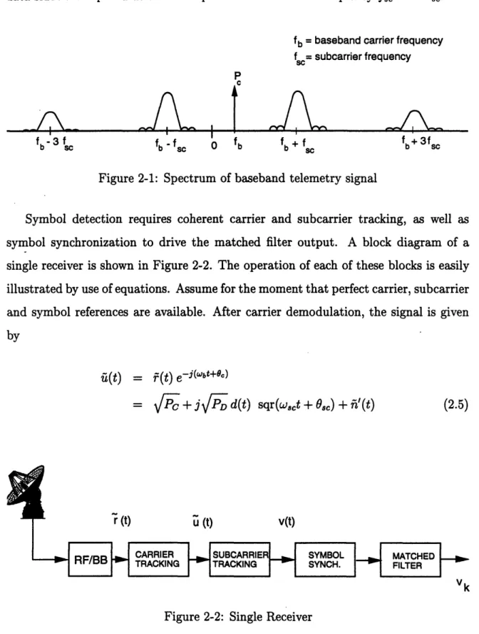
This complex notation will subsequently be used freely to represent a pair of baseband signals. The spectrum of the baseband signal fr(t) is shown in Figure 2-1. Note that

the signal consists of a residual carrier tone at frequency fb = 27rWb, surrounded by

data sidebands spaced at odd multiples of the subcarrier frequency f = 2rwsc.

fb = baseband carrier frequency

sc= subcarrier frequency

P

I

fb

fb-fsC 0 fb + fSC

Figure 2-1: Spectrum of baseband telemetry signal

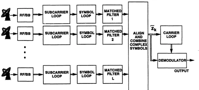
Symbol detection requires coherent carrier and subcarrier tracking, as well as symbol synchronization to drive the matched filter output. A block diagram of a single receiver is shown in Figure 2-2. The operation of each of these blocks is easily illustrated by use of equations. Assume for the moment that perfect carrier, subcarrier

and symbol references are available. After carrier demodulation, the signal is given by

i(t)

= (t) e-j(-bt+')

= vi

+

d(t) sqr(w

8

t +

Os)

+ W(t)

(2.5)

r(t) u (t) _v(t)

Vk Figure 2-2: Single Receiver

The data is contained solely in the imaginary part of the signal ii(t). Multiplying

f -3 _{b SC}f fb+ 3fsc

-this by the ideal subcarrier reference then yields the data stream alone, i.e.,

v(t) = m[ii(t)] sqr(w,,ct + 0C)

=

JPDd(t)

+ n'(t)

(2.6)

Finally, the symbol synchronizer provides timing for the matched filter, whose output

is given by

1 (k+l)T.

Vk =

-I

v(t)

= /PDdk + nk (2.7)

where k denotes the symbol index, and T8 is the symbol duration. Note that the noise output of the matched filter has variance N. The symbol SNR is defined as the mean of the matched filter output squared divided by its variance, and is equal

to 2PDTs/N, in the case where ideal references are available.

2.2 Symbol SNR Degradation

In practice, perfect references for all three stages of synchronization are not available. Carrier and subcarrier tracking loops are used to perform the demodulation, and a symbol synchronization loop is used to obtain symbol timing. Synchronization errors in each of these three loops thus result in an SNR at the matched filter output which is less than the ideal case. Symbol SNR degradation is defined as the ratio of the actual achieved symbol SNR to the ideal symbol SNR, and is used as a measure of receiver performance. A quantitative evaluation of degradation for a single receiver is given in [1], and the main results are summarized here.

In the presence of phase errors in each of the three loops, the matched filter output

is given by

= /jddk C, CS, Cy + nk (2.8)

where ₀

,

,, sy are the carrier, subcarrier, and symbol phase errors in radians, respectively, and the C factors are the signal reduction functions for each of the three loops. Note that the total signal reduction function can be factored into three separate terms, but the three phase errors are, in general, non-independent. The symbol SNR conditioned on the phase errors of the three loops is then given by

2PdT8

c

2

c

2 c2

SNR'

c2C2C2 (2.9)

The unconditional SNR is found by taking the expectation of (2.9) with respect to the various phase errors. The tracking performance of each of the three loops is a function of its respective loop SNR, which is defined as the inverse of the steady-state phase error variance. The loop SNRs for the carrier, subcarrier, and symbol loops are respectively given by

PC = PD

_B

(1 +

₂

1 (2.10)

E

/No

Pse = 1 + 2E/N) (2.11)

No F\ •aNo E (2.12)2

y 27rWB ( + i + Ef (v)] )

where Bc, B,, and Bsy are the carrier, subcarrier, and symbol loop bandwidths, respectively; Wsc and Wsy are the subcarrier and symbol windows; Es is the symbol energy, given by E, = PDTS; and Erf(x) is the error function, given by Erf(x) =

2/i f' e- 2_{dw. In expressing Pc, it has been assumed that a Costas loop is used for}

carrier tracking. The second moments of the reduction functions are related to the loop SNRs by the following:

C = 1 [1+ (2.13)

4 2 4 1

C2,

=

-1

+ __

~

(2.14)

C2

1 -

+

2

(2.15)

7r py 47r2 Psy,

where x denotes expectation of x, and Ik(x) denote the modified Bessel function of order k. The first moments of the subcarrier and symbol reduction functions will be needed in later analysis, and are given by

C,

= 1- /

2

₂

_(2.16)

Cy = 1- 2--1 27p (2.17)

Thus, the degradation for a single receiver is given by

D = C2 C2c C2y (2.18)

where C2_{, C2, and C2y are found by combining (2.10) - (2.12) with (2.13) - (2.15).}

2.3 FSC and CSC Arraying Techniques

We now provide a brief introduction to the full-spectrum combining and. complex symbol combining arraying schemes, which are described in detail in [2]. Each of these techniques will be treated in more depth in subsequent chapters; here, we merely provide a functional overview to illustrate the basic concept of arraying, and to point out the main differences between the two schemes.

2.3.1 Full Spectrum Combining

Full-spectrum combining is conceptually the more simple of the two schemes being considered. A block diagram of FSC for an array of L antennas is shown in Figure 2-3. Following down-conversion to baseband, each signal is delayed by some amount

.

I INTEGRATED DEMODULATOR I

I ,I - I- I I ,I

Figure 2-3: Block diagram of full-spectrum combining

The quantities ri can typically be computed in advance from the spacecraft trajectory and automatically adjusted over the course of a tracking pass. The delayed baseband signal from the it h antenna is given by

fi(t)

=

Vc

e(jWbt+Gci) _{+ jV/D d(t) sqr(w,,t +}

_{0,c)e(jibt+c)}

_{+ i,(t) (2.19)}

Note that the signals are aligned in time, but that the carrier phases 8c are not necessarily the same. Before the signals may be added coherently, L- 1 of the signals must be phase-rotated. We will designate antenna 1 as the reference antenna, such

that

fi(t)

must be rotated by an amount li - 8 for i = 2... L. Estimates

of the relative phases, li, are computed in real time by correlating each signal with

rl (t). Note that the combining block and the carrier loop perform distinct but related

functions: the former compensates for the differential phase between the various signal pairs, while the latter tracks the component of the phase common to all the signals.

For now, assume the desired phases li are estimated perfectly. Each signal is phase-rotated by the appropriate amount and multiplied by some pre-specified weight (

0/i, and the resulting signals are summed coherently, i.e., L

rcmb(t) =

E

i i(t) ejli

(2.20)

i=l L

r=

ej(w~bt+°1)Y

(V

+

ij

P d(t) sqr(wsct

+ Osc))

i=l

Finally, the combined signal is tracked by one carrier, subcarrier, and symbol loop, yielding an arrayed symbol stream given by

L L

Vkcomb=E pjV dk+ EZ nki (2.22)

i=1 i=1

where we have assumed perfect synchronization at each of the three stages. It is shown in [1] that when the noises from distinct antennas are independent, the SNR of the above expression is maximized if the weighting factors are chosen to satisfy the condition

PP No,

Pi Njo (2.23)

in which case the ideal combined SNR becomes 2PDjT L SNR b 2PDT

Eyi

(2.24) No_{0 1} i=1 2PDITs 2 GA (2.25)

N.,

where yji = P _PD N0o The factor GA is known as the arraying gain. Typically, antenna

1 N,

1 is specified to be the antenna with the strongest signal (i.e., the highest PT/No). The arraying gain then describes the increase in SNR over that achievable with any single antenna in the array. For the case of uncorrelated noises, we see that the effective P of the combined signal is equal to the sum of the Pa's of the individual antennas.

2.3.2

Complex Symbol Combining

Figure 2-4: Block diagram of complex symbol combining

A block diagram of complex symbol combining for an L antenna array is shown in Figure 2-4. Here, the baseband signals are tracked by separate subcarrier and symbol loops before the carrier is coherently demodulated. Thus, the baseband signal from

the ith _{antenna is first multiplied by the subcarrier reference from the ith subcarrier} loop, i.e.,

iii(t) = i(t) sqr(w t +0,,) (2.26)

= Vi e(j'wt+ci) sqr(wct +

8.)

+ j

A d(t)

e(jwbt+°ci ) _{+ i'(t)}

_(2.27)

where, once again, we have assumed perfect subcarrier reference for simplicity. This signal is then passed through a matched filter, whose timing is obtained from the ith

symbol loop, yielding a carrier-modulated symbol stream given by

zk =

VP

e( bk_{T.+i) dk + nk (2.28)} where we have implicitly assumed that the carrier phase is nearly constant over one

multiplied by the subcarrier reference integrates to zero.

These complex baseband symbols are then transmitted to a central location where they are phase-aligned, weighted, and combined, as in the case of full spectrum com-bining. The combined signal is thus given by

L L

Zkco.b = e(bkT+0cl)

E ,,

/

dk + i n 'r (2.29)

i=l i=l

A baseband Costas loop is finally used to demodulate the carrier, and the arrayed symbol stream is given by

Vkcmb-E = p

i

sVfi jdk + E/pi nk. (2.30)

i=l i=

Once again, when the noise at separate antennas is independent, the SNR of (2.30) is maximized by setting the weighting factors according to (2.23). The ideal SNR of the arrayed telemetry is then given by (2.25).

2.3.3 Comparison of FSC and CSC

We have seen that the "ideal" symbol SNR is the same for full spectrum combining and complex symbol combining in the absence of correlated noise. This result follows from intuition; if demodulation and combining can be achieved perfectly, it should not matter in which order the various processes take place. The same reasoning holds for the correlated noise case: the ideal symbol SNR will be different from (2.25), but will be independent of which scheme is used.

The performance of the two techniques will, however, be different when synchro-nization losses are accounted for. Note that when telemetry is arrayed, synchroniza-tion losses arise from imperfect carrier, subcarrier, and symbol tracking, as well as errors in phase-aligning the signals. In full-spectrum combining, the loop SNRs of each of the carrier, subcarrier, and symbol loops are increased by arraying the signals. By contrast, only the carrier loop SNR enjoys the benefit of the arraying gain in com-plex symbol combining. In addition, the subcarrier and symbol loops must operate

in the absence of carrier lock for CSC, resulting in a further reduction in loop SNR1. Thus, losses due to subcarrier and symbol tracking are higher for complex symbol combining than for full spectrum combining. Differences in the method of combining similarly lead to different synchronization losses.

Symbol SNR degradation is used as a measure of relative performance for the two schemes. Similar to the case of a single receiver, degradation is defined as the ratio of the actual to ideal arrayed symbol SNR. Degradation for each of these arraying schemes has been analyzed in past literature for the case where the noise encountered at the various antennas are independent [2]. We will later extend this analysis to include the case of arbitrary noise correlation between the various antennas.

We note that the effects of correlated noise on arraying can be separated into two different but related factors. The first is the ideal arraying gain, which will

be dependent on the correlation properties of the noise itself, but independent of which scheme is used. The second is the degradation, which will depend on the noise properties as well as which arraying technique is used. Each of these will be analyzed in turn in Chapters 4 and 5; we presently turn to a discussion of radio sources to develop an appropriate model for correlated noise due to a common background.

1Modified subcarrier and symbol loops have been developed for use with complex symbol com-bining. These loops utilize information in both the I and Q components of the complex signal to recover some of the loss in loop SNR due to the absence of carrier lock. The relevant details will be presented in Chapter 5, where CSC is analyzed in further detail.

Chapter 3

Modeling of Background Noise

This chapter covers basic concepts needed to characterize noise due to radio sources. The first section presents terminology used in radio science to describe broadband sources, and shows how the effect of background noise on a single receiving system can be accounted for by an equivalent source temperature. In the second section, we consider the effect of a noisy background on a pair of antennas, using interferometry theory to compute the cross-correlation function of the received noise waveforms. Section three extends this analysis to a baseband receiving system, which will be assumed for the remainder of this work. Finally, section four presents the results of an experiment that was conducted to illustrate the basic principles outlined in this chapter.

3.1 Background Noise in a Single Receiver

In deep space communications, signals are generally assumed to be received through an additive white Gaussian noise channel. The noise level in a receiving system is commonly characterized by a system temperature, Ty,. The one-sided power spectral density of the noise is then given by No = kTsys, where k is Boltzmann's constant. Background sources such as planets are typically broad-band, and have an emission spectrum that is reasonably flat over a frequency range of interest. Receiving band-widths for deep space applications are typically no greater than 100 MHz, over which

the background noise can essentially be considered white. Thus, the noise level con-tributed by the background can be described by a background temperature, Tb, which measures the contribution of the source to the total system noise. Here, we show how this temperature can be computed from more physically informative characteristics of the source.

A radio source is generally described by its brightness distribution, B(O, 0), which has units of W/m 2_{/Hz/sr 1. The variables b and 0 indicate that brightness refers} to a particular direction; an arbitrary source may have some parts that radiate more strongly than others. The total strength of the source can be measured by its flux

density, S, which is equal to the brightness distribution integrated over the angular

extent of the source, i.e.,

S

=

JB(0,)dQ

(3.1)

where the integration variable Q denotes integration over a solid angle. Thus, the units of flux density are W/m2/Hz. Note that the flux density of a particular source

depends on its distance from Earth; the closer the source, the larger solid angle it subtends, and hence the larger the flux density becomes.

The noise level due to such a source as observed by a receiving antenna can be described by a background temperature, as discussed above, which is given by

Ae

Tb= 2k | B(,)PN(,)dQ (3.2) where Ae is the effective collecting area of the antenna, and PN(0, 0) is the normalized

antenna reception pattern. Thus, the contribution of a background source to total

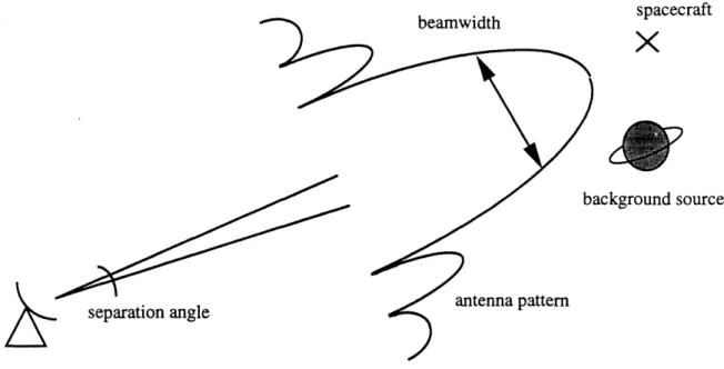
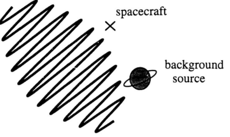
system noise depends on the strength of the source and its position in the antenna pattern. For telemetry applications, the antenna is pointed at the spacecraft, so the contribution of a given source varies with its angular separation from the spacecraft. This situation is depicted in Figure 3-1.

In the worst-case scenario, the source-to-spacecraft angular separation is zero or 1The unit sr stands for steradian, which is a measure of solid angle.

..- spacecraft

X

2

ackground source

/z

7

separation angle

Figure 3-1: Spacecraft and background source in common beam

negligibly small compared to the beamwidth of the antenna. The antenna pattern term, PN, then approaches unity over the integral, and

Ae

Tb

= 2k |

₌

_S

f B(/ , )dQ

(3.3)

_(3.4)

2k

An upper limit on the total system temperature that a source can contribute can thus be computed from the flux density of the source and the effective area of the receiving antenna.

3.2

Simple Radio Interferometer

We now turn to the properties of correlated background noise as observed by two antennas. Specifically, this section computes the cross-correlation function of the noise due to the source. A pair of antennas basically behaves as an interferometer, and computation of the cross-correlation function follows from fundamental principles of interferometry. We start by considering an oversimplified model for illustrative

purposes, and then gradually move to one that more accurately describes an actual receiving system. The discussion below provides a general idea of the issues involved, and is not meant to be a rigorous treatment of the subject. A more thorough analysis can be found in a text on radio astronomy, such as [6].

Consider two antennas tracking a distant radio source, as depicted in Figure 3-2. The received noise waveforms are filtered by some front-end filter centered at

/ / /

/ /

/

D

pa/

Figure 3-2: Antenna pair tracking distant source

frequency fo. Since the received noise is white, the form of the correlation function is determined solely by the characteristics of the front-end filters. The cross-correlation function of the noise waveforms is defined as

R(r) = E[n

1

(t)n

2

(t

-

r)1

(3.5)

Note that n₁(t) and n2(t) can be taken to be the noises due to the background source alone or the total noise waveforms at antennas 1 and 2, since the noises due to front-end electronics are indepfront-endent. In the case of a simple point source, the received waveforms are identical except for some geometric delay r9. The cross-correlation function then takes the form

where G(r) is some function determined by the shape of the front-end filters. For example, in the case of a rectangular passband of one-sided bandwidth B, G(t) would be given by sin rBt/7rt. Under typical conditions, the receiving bandwidth is much smaller than the center frequency. Thus, the correlation function consists of a slowly-varying envelope modulated by a rapidly-slowly-varying sinusoid at the center frequency of the passband. The latter is referred to as the delay pattern, while the former is known

as the fringe pattern.

The geometric delay is due to the difference in path lengths from the source to each of the two antennas. From Figure 5, it is readily seen that rg can be expressed

as

D sin 0

9 (3.7)

C

where D is the separation baseline between the two antennas in meters, 0 is the angle as shown in Figure 5, and c is the speed of light. The correlation function thus has both a temporal and spatial dependence. To consider the effect of varying the angle 0, the above quantity can be expanded in a first-order Taylor series about some reference

position 80:

T-g -(sin 80 + ' cos 80) (3.8)

where 0 = 8o + 8'. Now let one of the signals be delayed by some amount rgo equal to the geometric delay at angle 00. Inserting (3.8) into the shifted cross-correlation function yields

R(r, 9') = G(r -

-'

cos o8)

cos 27rfo(r - -'

cos

8o)

(3.9)

C C

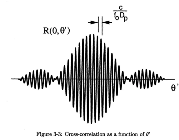
This function is plotted as a function of 0' for a fixed value of r in Figure 3-3. Note that the quantity Dp = D cos 00 is the projected baseline in the direction of the source. (See Figure 3-2) The spacing between the oscillations is given by w = c/(foDp). This quantity, known as the fringe spacing, has important implications for the measured noise correlation due to an arbitrary source. Recall that the expression given in (3.9) was developed for a point source. In general, the correlation function due to a source of non-infinitesimal size will have to be computed as an integral of the above

C

f_-

n

R(O, 0')

II

Figure 3-3: Cross-correlation as a function of 0'

expression over the angular extent of the body. If the body being observed subtends many fringe cycles, then the measured correlation tends to zero due to the averaging effect of the sinusoid. Such a body is said to be resolved by the array.

Figure 3-4 shows the interference pattern formed by two antennas against a sky background. Here, it can be seen that the angular size of the source relative to the fringe spacing is what determines whether or not the source is resolved by the array. For a given source and observation frequency, the length of the baseline determines the degree to which the source is resolved. Consider a source having an angular radius of R8 radians observed at some frequency f Hz. In the long baseline limit, where Dp > c/(foR.), the fringe spacing is extremely small compared to the size of the source, and the noise correlation tends to zero. By contrast, for extremely short baselines, such that Dp < c/(foRs), the effect of the averaging sinusoid is negligible, and the noise correlation is maximized. Thus, the degree of noise correlation observed depends heavily on the geometry of the array. This point is stressed in [3], where it is

stated that the more compact the array configuration, the greater the impact of the

background body on the array. As an example, consider observing Jupiter at S-band

,acecraft

background source

KY

estimate p.hase

Figure 3-4: Fringe pattern against sky background

(2.3 GHz). The planet's angular size varies with its distance to earth, but a typical value is 10-3 radians. An antenna separation on the order of a few hundred meters would thus be required to observe a measurable degree of noise correlation.

At this point, a more general expression for the cross-correlation for an arbitrary source can be presented. It is shown in [6] that R(r) can be expressed as

R(r) = G(is) aiek

J

J

PN

(p)PNk

(o)B()

cos 27rf0() - Bik * c/c)dQ (3.10) where a is a unit vector specifying the direction, PN (a) and PNk (a) are the normalized

antenna reception patterns in the direction a, Ae,, and Aek are the effective areas of the two antennas, B(a) is the brightness of the source in the direction a, Bik is the baseline vector, and dQ2 is the element of solid angle over which the integral is taken. Note that the effect of spatial variations on the delay pattern term, G, has been neglected. This approximation is justified if the received signals are narrowband, since the delay term then varies much more slowly than the fringe term. This can be seen graphically in Figure 3-4; over the integral, the envelope of the interferometer reception pattern is essentially constant, while the sinusoidal component is more quickly-varying. In addition, it has been assumed that the correct geometric delay has been inserted to compensate for the differential pathlength to the source.

A useful quantity known as the complex visibility can be defined as

V

=VIe"f

=f lPNi

()PN,()B(a)e

2B /c

dQ

(3.11)

After some manipulation, R(r) can be expressed as

R(r) =

G(T)IVI

cos(2irf

-

)

(3.12)

2

= aG(r) cos(2irf - v) (3.13)

where A,e and Ae2 are the effective collecting areas of the two antennas. The variable a = 2 IVI has been introduced for notational convenience, and is the cross power spectral density between the two noise waveforms, having units of W/Hz. Note that

V has the same units as flux density (W / m2 / Hz). In the upper limit, all terms in the integrand of (3.11) except the source brightness approach unity, and V approaches

the flux density of the source being observed.

3.3 Cross-correlation for Baseband Signals

As discussed in Chapter 2, we are assuming that all processing takes place at base-band. Thus, here we compute the cross-correlation for the equivalent baseband

sig-nals. Recall that each bandpass RF signal is down-converted by two oscillators in phase quadrature, resulting in a pair of baseband signals. Consider representing the bandpass signals as

nl (t) = xl(t) cos wt - yl (t) sin wot

n2(t) = x2(t) cos ot - y2(t) sin

wot

(3.14)

where w, = 2rfo. Let nl(t) and n2(t) be bandpass Gaussian random processes cen-tered in frequency at f, and having spectral levels No and No₁ 2, respectively. It is shown in [4] that xi (t) and yi(t) are then lowpass Gaussian random processes with spectral levels 2N,,, and that xi (t) and yi(t) are uncorrelated for all t (i = 1,2). Expressing the cross-correlation function in terms of these lowpass processes, we find

Rnl,n2(r) = E[n1 (t)n2(t - r)]

1 1

= (Rx₁,x2(7) + Ryl,y2(T)) COS Wo + -(R1,x2() - Ryly2()) cos(2wt -

wr)

2 2

+ Il(Ryl,2(r) - Rl,y

2

(T)) sin wor- (Ryl,x2(r)

+ Ril,y

2

(T)) sin(2wt - wor)

2 2

(3.15)

This can now be related to the form of the cross-correlation function found from section 2. Assuming the fixed delay is not inserted, we know Rnl,n2 takes the form

Rnl,n2(r) =

aG(r

-

g)

cos(wr -

)

= aG(r - rg) cos cos wr + aG(T - rg) sin ), sin WoT (3.16)

Thus, the equivalence between (3.15) and (3.16) holds only if the following symmetry conditions are true:

R:11,.2( ) = Ryl,y2(r) = G(r

-

r₉

)cosX

Rll,z2(r) = -Rly2(r) =

cG(r

- Tg)

sin

(3.17)

At this point, it is straightforward to show that the cross-correlation of the complex baseband signals will take a similar form:

R;,,r2(r) =

E[Ri(t)hf(t

-

r)]

= aG(r - rg)e0l2

(3.18)

The phase '2 accounts for the visibility phase X, plus any phase difference introduced

by the local oscillators at the two antennas. After down-conversion to baseband, one of the complex signals is delayed by an amount r9 to compensate for the geometric

delay at some position 00. In practice, this delay is computed based on the position of the spacecraft. This delay will, in general, be different from the quantity r9in (3.18), since the background source is at a slightly different position than the spacecraft. However, we will assume that this "residual delay" is very small compared to the inverse filter-bandwidth. Thus, (3.18) becomes

RE.l,62(-) a oG(7)ej'l 2 (3.19)

where G(r) is some lowpass waveform centered at r = 0. We shall see in the next chapter that the difference between the relative noise phase 12 and relative signal

phase 12 (defined in Chapter 2) is an important parameter in determining the ar-raying gain. We denote this quantity by l12 2 -

012-Note that in deriving (3.19), we have considered the noise generated by the back-ground source only. As mentioned in Chapter 2, however, the additive noise present with the telemetry signal is actually composed of background noise plus that due to receiver electronics. Nevertheless, (3.19) can still be used to describe the cross-correlation, since the noises due to electronics at distinct receivers are independent, Furthermore, it should be noted that (3.19) closely resembles the form of the

auto-correlation function for the complex baseband noise observed at a single antenna. Specifically, for noise with a one-sided power spectral density level of No W/Hz, the autocorrelation is given by

Rn(T) = E[n(t)n*(t - )] = NoG(T) (3.20)

Let the correlation coefficient between the noise at two antennas be defined as

P = 4;< (3.21)

An upper limit for p is found by assuming that the source is in the peak of both antenna patterns, and is very small compared to the fringe period. In this case,

/A

1

2 S

2

=

k

/S

82

(3.22)

where T1 and T2 are the system temperature increases due to the source at the individual antennas. Combining (3.22) with (3.21) yields

P =V T1T2 (3.23)

where T1 and T1 are the total system temperatures at the two antennas.

3.4 Experimental Data

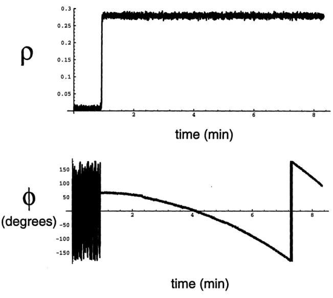
To illustrate the basic concepts of noise correlation due to a common background, an experiment was conducted as part of this thesis using two of the DSN's antennas at the Goldstone, California complex. Observations of 3C84, which is a broad-band radio source, were made at S-band (2.3 GHz) from a 70-m and 34-m dish antenna. The signals were down-converted to baseband, filtered to a one-sided lowpass bandwidth of 115 kHz, sampled at the Nyquist rate of 230 kHz, and recorded on magnetic

tape. The recorded signals were then processed on a Sun workstation to compute the correlation as a function of time. Figure 3-5 shows the normalized correlation p and the measured visibility phase over a period of approximately 8 1/2 minutes. A 0.1 second integration time was used to estimate the correlation for each point. The sharp transition approximately 1 minute from the start indicates the time one of the antennas moved from off the source to pointing at it.

0.3_r 0.25 0.2 0.15 0.1 0.05 z 4 b U

time (min)

150 100

(degrees)

-50 -100 -150

time (min)

Figure 3-5: Experimental correlation data for 3C84

For the 70-m antenna, the source temperature was measured to be T = 35.8K, and the total system temperature (including the source) was measured at T₁ = 50.3K. The corresponding temperatures for the 34-m antenna were T82 = 7.86K and T2 =

40.96K. Note that the contribution of the radio source to the 70-m system

temper-. . .

-uu(

- - --- A- -~~r Lc. - -- .·- - .- A-- YI-

--I - - -- - - - -- - .-

ature is roughly four times greater due to the ratio of the collecting areas. Based on these numbers, the upper bound for the correlation coefficient, using (3.23), is

p < 0.37. The mean correlation coefficient measured is approximately 0.26. This

difference can be explained by the "resolving" effect. The physical separation be-tween the two antennas is 500 m, from which we conclude the fringe spacing, given by w = c/(foDp), is on the order of 3 x 10- 4 radians. The angular size of 3C84 is comparable to this, being approximately 1 x 10- 3 _{radians. Thus, some decrease in} the correlation is expected due to averaging over the fringe oscillations.

The above example illustrates how physical parameters such as source size, base-line length, observation frequency, and source and system temperature can be com-bined to form a rough estimate of what degree of noise correlation can be expected for a given scenario.

Chapter 4

Full Spectrum Combining

Performance

This chapter contains a quantitative evaluation of full spectrum combining perfor-mance in the presence of correlated noise. In Chapter 2, it was noted that both the ideal arraying gain, GA, and the arraying degradation, D, are different when corre-lated noise is present relative to the case of uncorrecorre-lated noise. Section 1 evaluates

GA in terms of the noise correlation parameters pij and Oij described in the previous

chapter. Section 2 then computes the degradation due to imperfect synchronization for full spectrum combining, Df,,. We will see that a major difficulty caused by the noise correlation is the issue of phasing the array. The conventional phase es-timation scheme, discussed in [1] and [2], is described, and a modified method to offset the problems caused by noise correlation is proposed. An expression for the arrayed symbol SNR, taking into account phase-alignment and demodulation losses,

is then presented, and the degradation is computed. Finally, the analytical results

are compared to values obtained by simulation in Section 3.

4.1 Ideal Arraying Gain

Consider an array consisting of L antennas. Recalling the signal format for deep-space telemetry presented in Chapter 2, the complex baseband signal from the it_{h antenna}

can be expressed as

ri(t) = si(t + (t)

V ei(b

+ '

_{) +}

_{jPid(t) sqr(wsct}

₊

_sc)e

j

_(wbt+

°

_ci)

₊

_{ii(t) (4.1)}

From (2.21), the combined baseband signal for full spectrum combining can be ex-pressed as

rcomb (t) = Scomb(t) + Acomb(t)

L

= E pi (Si(t) + ni(])) ejoli i=l

ei(Wbt+'1) B'i (

c+

jPDj

d(t) sqr(ct +

0S))

(4.2)

L

wai=lh

where we have assumed the ith signal has been phase-rotated by an amount 1li to

compensate for the difference in carrier phase between the 1t _{and ith antenna. If} all the noise processes hi(t) are uncorrelated, the SNR of the combined signal is maximized if the weights f3i are chosen to satisfy the condition

PT, No,

for i = 1 ... L. Note, however, that this is not the optimal choice of weights in the case of correlated noise waveforms. Furthermore, the optimal choice of phases used to array the signals is not necessarily the relative signal phases, li. Using the phases 01i will certainly maximize the arrayed signal power, but not necessarily the ratio of signal to noise power, which is the relevant criteria for optimization. The problem of optimal combining weights and phases for signals with correlated noise has been analyzed in [7], where the results are applied to an array of antenna feed elements. However, computation of these weights requires knowledge of the pairwise correlations between the noises, aijeJiji A scheme can be devised to estimate the required parameters in

real time and modify the weights accordingly, but would significantly complicate the problem. Our goal, instead, is to determine the performance impact of the correlated

noise assuming the traditional combining scheme is used. The total combined signal power, PT, is given by

PT E[Omb(t)] E[SoCb(t)] (4.4)

If the weighting factors are chosen according to 4.3, the combined signal power be-comes

L L L

PT = PT1

5

+

E'

Yitj

)

(4.5)

i=l j=l

where =

-

A N'

The one-sided power spectral density of the real and imaginary parts of the com-bined noise is given by

No- _2BE[icomb(t) fncomb(t)] (4.6)

where B is the one-sided bandwidth of the noise waveforms. Note that the factor

of two in the denominator of (4.6) results from the fact that the real and imaginary parts of the noise each has half the power of the complex noise. From the definitions of power spectral density and cross power spectral density, it follows that

E[ii(t)hfi(t)] = 2NoB

(4.7)

E[Ai(t)ij(t)] = 2aoije0ZiB (4.8)

Equations (4.6), (4.7), and (4.8) can be combined to find the power spectral density of the combined noise, yielding

L L L

No

-N yi

+

E E

y

pije

(i-i

)

_(4.9)

The PT/No of the combined signal is thus given by

PT PTi

N

0

_{N. N.,}

N

0

_{5-]-=1 q-}

a

₊

+E

₊

+

L

z,

i

_I

L

Pzi

Pij

e''i

(4.10)

where Obij = OP - ij, as defined in Chapter 3. The parameters pij and V/ij describe the relevant statistics for the noise correlations between the various antenna pairs, and determine the correlated noise impact on the ideal arraying gain.

The combined signal is finally processed by a single carrier, subcarrier, and symbol loop. Assuming perfect references at each of these three stages, the symbol SNR of the arrayed signal becomes

2PD,

(El )

SNRideal =

Nol Rsym

Z=

17yi + Z=~ E= ji= (YiYj) /2pij e3i

No2PDm GA (4.11)

No, Rsym

where GA is the ideal arraying gain due to combining the signals. Note that setting all the noise correlation coefficients pij to zero results in GA = yL=1 i, which is the ideal arraying gain in the case of uncorrelated noises, as discussed in [1].

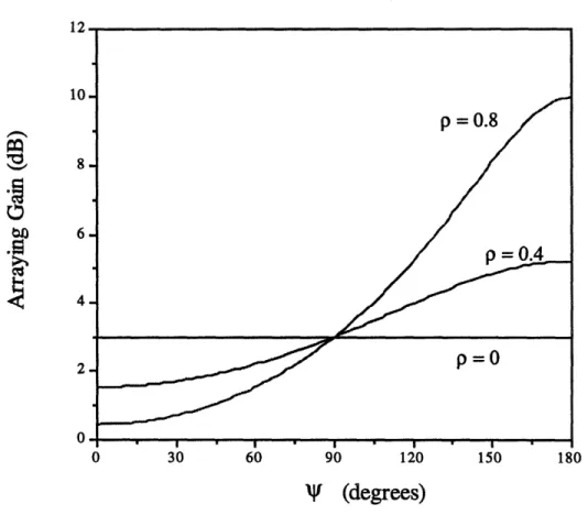
Further note that the ideal arraying gain in the presence of correlated noise can be higher or lower than the uncorrelated noise case, depending on the phases Oij. The intuitive reason for this can be understood by considering an array of two equal antennas (i.e., 1 = 72 = 1.) Figure 4-1 shows values for GA for two equal antennas as a function of p and A. For p = 0, the ideal arraying gain is a constant 3 dB, as expected. Now suppose the noises have some nonzero correlation coefficient p, and some correlation phase /bn. If ?i = 0°, then the phase difference of the spacecraft signal as observed by antennas 1 and 2, X, is equal to the noise correlation phase qb" . Thus, phase-aligning the two signals also phase-aligns the correlated component of the noise. The noise from the background source adds maximally in phase, and the combined noise power increases. Thus, the combined SNR decreases, and hence the arraying gain falls below 3 dB. By contrast, if 0 = 180°, phase-aligning the signal

results in combining the correlated component of the noise 180° _{out of phase. Thus,} the noise combines destructively in this case, and the arraying gain is now greater than 3 dB. For intermediate values of

4,

the arraying gain varies continuously from

its minimum value at

4'

= 0° to its maximum at

4'

= 180°.

Ideal Arraying Gain

1-0

I

co 0 30 60 90 120

v

(degrees)

150 180

Figure 4-1: Ideal arraying gain GA for various p,

4

4.2 Symbol SNR Degradation

In practice, perfect phase alignment and ideal carrier, subcarrier, and symbol refer-ences are not available. Some degradation in the arrayed symbol SNR is therefore incurred due to synchronization errors. To quantify the degradation, we first find the set of density functions for the phase alignment errors Abli jli - li, i = 2 ... L. This set of functions is then used to compute the PT/No of the arrayed signal. Adding in losses due to carrier, subcarrier, and symbol tracking, the symbol SNR at the

matched filter output can be computed. Finally, comparing the actual symbol SNR to the ideal symbol SNR given by (4.11) yields the degradation for full spectrum combining.

4.2.1 Antenna Phasing

A set of phase estimates ~li for i = 2... L are needed to align signals 2... L with signal 1. In the description of FSC given in [2], the phase difference between §s(t) and s1(t) is estimated by filtering the two signals to some lowpass bandwidth Bip Hertz, multiplying them, and averaging their product over Tcorr seconds. The phase of this

complex quantity is then computed by taking the inverse tangent of the ratio of the

imaginary to real parts. A block diagram of this scheme is shown in Figure 4-2.

r1

ri₁

Figure 4-2: Conventional phase estimator

The complex product of the baseband signals after averaging, Z, is given by

Z I

T1

Wp

+

lpl(t))

(lpi(t)

+lpi

(t))

=

(P/PC

+

PD

1

PDHH))eT

( (t) +

lp(t)

i',(t))

dt

(4.12) where H is given by H =(4 2 M 1 (4.13) i odd

and M is the highest harmonic of the subcarrier passed by the lowpass filter. The term ii8,(t) is composed of signal-noise terms in the product and has zero mean.

Note, however, that the noise-noise term, ilp,,(t)p (t), does not necessarily have zero

mean, due to a possible correlation that exists between the two noise waveforms. The expected value of this noise product can easily be computed from the cross power spectral density of il(t) and ii(t); thus,

E[Z]= (PCPc +

P

+

2

pPD/H)ei1li

pljNjN

0

"Bpe1

(4.14)

Since 'i is not necessarily equal to 1ji, the noise product introduces a "bias" to the estimate of the relative signal phase. This situation can be represented pictorially in Figure 4-3. The complex quantity E[z] can be thought of as a vector sum of a

signal-N

Figure 4-3: Complex correlation vector

to-signal correlation, S, and a noise-to-noise correlation, N. Note how the presence of the noise vector biases the measurement of the phase of the complex correlation. The relative magnitude of these vectors is given by

_ 2

1-

Bp

(Pli

l

No1/2

IN} - 2pjj Bip

k.No:

Nj

+ PD PDNo 1/2

N.,

N.,

For typical parameters, even relatively modest levels of noise correlation can lead to a substantial biasing effect in estimating the relative signal phase. For example, consider

correlating two signals each having a PT/No of 20 dB-Hz with a 1 kHz correlation bandwidth. Even if all subcarrier harmonics are included in the correlation, making

H = 1, a correlation coefficient as low as p = 0.1 makes the ratio in (4.15) equal to

0.5. The phase estimates are then influenced more by the relative noise phases i than the desired quantities li, leading to a high amount of degradation in combining the signals. A practical implementation of full spectrum combining therefore requires a modified phase estimation algorithm if correlation levels encountered will generate significant biases.

The method of phase estimation shown in Figure 4-4 can be used for this purpose. Here, each signal is filtered to some bandpass bandwidth Bbp, and an additional com-plex correlation is performed between the resulting waveforms. The center frequency of this filter is chosen so as to not capture any energy from the telemetry; this can be

,\

Figure 4-4: Modified phase estimator

accomplished by locating the filter at an even multiple of the subcarrier frequency, for example. After scaling the noise-only correlation by the ratio of the lowpass

to bandpass bandwidths, this quantity provides an estimate of the contribution of the noise to the total correlation. The bandpass correlation can then be subtracted

from the lowpass correlation to compensate for the mean correlation vector IN. The compensated correlation can thus be expressed as

Z =

(VPCP0

+ VPDlPH)PHei1Tli

+

(i(8 (t) + filpi(t)

nlpi(t))

dt

BIp Tcorr1

J

bp(t)i* (t) dt

Bbp Tcorr h bp i

(IP\i + PdlPH)e kli +

N

(4.16)

where the the noise term N now has zero mean. The phase estimate is then found by taking the inverse tangent of the ratio of the imaginary to real part of (4.16), i.e.,

itan-1

[(

t

PDlPDH)

sinli+NQ

(4.17)

(PC 1PC + PD1PDi H) cos i + N

where N1 and NQ are the real and imaginary parts of N, respectively. Note that

although N and NQ have zero mean, their joint statistics are still influenced by the

correlation between i1(t) and hi(t). These statistics are analyzed in Appendix A, and the density function for the phase estimation error Aq0li _li - li is derived.

In [2], a quantity known as the correlator SNR is introduced, defined as E[Z]E* [Z]

SNRor, = E[ZZ*] E[Z]E*[Z] (4.18)

The correlator SNR is a measure of the spread of the phase error density pO(/A0li), and is inversely related to the variance of the phase error. In [1], where FSC is analyzed for independent noises, it is shown that the phase error density can be expressed solely in terms of the correlator SNR. For the correlated noise case, the density is given in Appendix A in terms of the correlator SNR and the correlation parameters

Pli and bli.

Figures 4-5 - 4-7 show the density function po(Aq5) for various values of p and V. The signal parameters chosen for these curves are (PT/No)l = (PTINo)2 = 25 dB-Hz, A = 90 deg, with seven subcarrier harmonics included in the correlation. The correlator parameters are Bip = Bbp = 15 kHz, and Tcor = 3 seconds. Note that even for a noise correlation as high as 0.4, the density function looks remarkably like that of the uncorrelated noise case. Simulations were performed for the same parameters, and densities collected for the measured phase estimates. These results are shown with the analytical curves in Figure 4-8.

p (phi) 2

1.5

50 -25 0 25 50 75

p=-Figure 4-5: Phase estimate density

p(phi) 2 1.5 1 0.5 ... . [C ' -phi -75 -50 -25 0 25 50 75

p = 0.4,

=

0 degrees

p (phi) 2 1.5 0.5 -75 -50 -25 0 25 50 75

-p = 0.4,

v

= 90 degrees

2 1.5 1 0.5 -75 -50 -25 0 25 50 75

p = 0.4,

N

=

_{45 degrees}

p(phi) -50 -25 0 25 50

p = 0.4, Nf = 35degrees

p (phi) 2 1.5 1 0.5 -75 -50 -25 0 25 50' 7 50 5 75 pni

p = 0.4,

v

= 180degrees

Figure 4-6: Phase estimate densities

phi - w p(phi) _ _ _ _ _ _ - ' hi ... , nhi -L

--p(phi) 15 1 0.5 1.5 0.5 -75 -50 -25 0 25 50 75

-p=0.8,

=0 degrees

-75 -50 -25 I 0 25 50 75

-p = 0.8,

= 45 degrees

p(phi) 2 1.5 0.5 p (phi) 1.5 0.5 -75 -50 -25 0 25 50 75 -75 -50 -25 0 25 50 75

p = 0°8,

v

= 90 degrees

p

= 0.8, ij = 135degrees

p(phi) 1 1 0o.5 -75 -50 -25 0 25 .... 50 50 75 phi

p = 0.8,

v

= 180 degrees

Figure 4-7: Phase estimate densities

- l p (phi) - I " ~~~~~ _ >4 .... . . .. ""'_\1\: ,hi i\ ... 1rl I; -,i I ...