The curious case of urban heat island : a systems analysis

The Curious Case of Urban Heat Island:

A Systems Analysis

By Joseph H. Yang

B.A.Sc. Applied Science and Engineering University of Toronto, 2000 MASSACHUSETTS INSTITUTE OF TECHNOLOGY

OCT 2562016

LIBRARIES

ARCHIVES

SUBMITTED TO THE DEPARTMENT OF SYSTEM DESIGN AND MANAGEMENT IN PARTIAL FULFILLMENT OF THE REQUIREMENTS FOR THE DEGREE OF

MASTER OF SCIENCE IN ENGINEERING AT THE

MASSACHUSETTS INSTITUTE OF TECHNOLOGY JUNE 2016

2016 Joseph H. Yang. All rights reserved

The author hereby grants to MIT permission to reproduce and to distribute publicly paper and electronic copies of this thesis document in whole or in part in any medium now known or hereafter created.

Signature of Author:

Certified by:

Accepted by:

/

I

Signature redacted

D a ent f SysteMDesign ar A 1gement

Wy 0O, 2016

________

Signature redacted

Le e Norford sr iIof ing 8 h Jogy

7(AhCesislui rrvimr

Signature

redacted

Pat Hale Director, System Design and Management Program

MIT Libraries

77 Massachusetts Avenue Cambridge, MA 02139 http://libraries.mit.edu/ask

DISCLAIMER NOTICE

Due to the condition of the original material, there are unavoidable

flaws in this reproduction. We have made every effort possible to

provide you with the best copy available.

Thank you.

The images contained in this document are of the

.best quality available.

The Curious Case of Urban Heat Island:

A Systems Analysis

Joseph H. Yang

Submitted to the Department of SDM on May 2 0th, 2016 in Partial Fulfillment of the Requirements for

the Degree of Master of Science in Engineering

ABSTRACT

This thesis provides insights into the urban heat island (UHI) effect using a model of the urban

microclimate that integrates the urban geometry, anthropogenic heat emission and the rural weather condition. The study builds upon the Urban Weather Generator (UWG), a numerical simulation program previously developed at MIT, incorporating such improvements as monthly disaggregation of ground sink temperature, Depart of Energy (DOE) commercial reference building templates, hourly schedule of building and non-building anthropogenic heat loads, and the development of an Excel user interface. Simulation generated from the updated model offers an explanation of the underlying mechanisms driving the UHI impact and the interactions between elements of the urban weather system. Based on the sensible energy flux transferred to the urban air mass, an UHI indicator to express the severity of UHI effect by the urban landscape is also developed to help urban planners estimate and mitigate the impact.

Thesis Supervisor: Leslie Norford Title: Professor of Building Technology

ACKNOWLEDGEMENT

I had the great privilege and fortune to have had a weekly session with Prof. Les Norford, my thesis supervisor, who trusted me with this project despite my limited experience and knowledge in building technologies and urban planning. It was a fantastic learning experience and I'm indebted to Les for bringing me on board and helping me to understand the nature of the problem.

I am grateful for the groundwork laid on the project by Bruno Bueno, who developed the model as part of his PhD thesis at MIT, and Aiko Nakano, who worked on the user interface for her Master's thesis, also at MIT. They both have graciously made themselves available to answer my questions, by phone calls and emails even though they no longer have commitments to the project.

Sometimes casual and short discussions make their way into the research and help to clarify issues. My discussions with Amir Aliabadi, Chris Mackey, and Xin Xu helped to identify needed improvements in the model and guide my thinking on what to incorporate.

Lastly, I'm grateful to have had the unwavering support from Janny throughout the academic year, who also provided proof-reading for this thesis. Without her ability to make sense of things that I couldn't articulate and provide stability in my daily life, this thesis would have turned out very differently. All models are wrong but some are said to be useful. Any errors in the model or the thesis reflect the limitations of the author, who nonetheless hopes the model and the insights in this report might provide value to others.

1

CONTENTS

1

4 The Urban W eather Generator ... 10

4.1 Urban M icroclim ate System ... 10

4.2 Urban Canyon Layer M odel ... 13

4.2.1 Urban Configuration ... 13

4.2.2 Energy Balance ... 15

4.2.3 Solar Radiation ... 16

4.2.4 IR Exchange Correction... 17

4.2.5 Hum idity...20

4.2.6 Urban W ind Speed... 21

4.2.7 Anthropogenic (Traffic) Heat Flux... 21

4.2.8 Soil Tem perature and Road Layers... 22

4.3 Urban Boundary Layer M odel... 22

4.4 Building Energy M odel...23

4.4.1 Energy Balance ... 23

4.4.2 DOE Reference Buildings... 25

4.4.3 DOE Building Elem ent Sizing ... 28

4.4.4 Building W aste Heat...29

4.5 Vertical Diffusion M odel...30

5 Case Study and M odel Validation ... 33

5.1 Validation of Urban W eather... 33

5.1.1 Com parison: BUBBLE ... 34

5.1.2 Com parison: CAPITOUL ... 34

5.1.3 Com parison: Singapore ... 35

5.1.4 Observations ... 36

5.2 Validation of Building Energy M odel ... 38

5.2.1 Boston Urban Configurations... 38

5.2.2 Sum m er Electricity Profile... 41

5.2.3 W inter Gas Profile...44

6 Findings & Insights ... 46

6.1 UHI M echanism... 46

6.2 UHI Im pact on Building Energy Costs... 48

6.3 Quantifying UHI... 50

7 Discussion...57

8 References ... 59

Append ix A UW G Program ... 61

Appendix B Building Electricity Validation (Boston, Sum m er) ... 66

2 TABLE

OF

FIGURES

Figure 4-1 Diurnal Structure of the Urban Boundary Layer... 11

Figure 4-2 Major Elements of UWG, showing Convective (Left) and Radiative (Right) Interface ... 12

Figure 4-3 Urban Area Characteristic Dimensions ... 13

Figure 4-4 Boundary Definition in UWG versions: Previous (Left) and New (Right)... 15

Figure 4-5 Air Emissivity Values per previous version of UWG...18

Figure 4-6 IR Transfer Characteristics at 1km height, MODTRAN ... 19

Figure 4-7 Non-BLD Anthropogenic Heat Schedule... 21

Figure 4-8 Ground Tem perature Variation ... 22

Figure 4-9 DOE Reference Commercial Building Types ... 25

Figure 4-10 Example of the Vertical Diffusion Model Temperature Profile ... 30

Figure 4-11 Urban M icroclim ate W orkflow ... 31

Figure 5-1 BUBBLE Comparison: Bueno (2013) (left) vs. new UWG (right) ... 34

Figure 5-2 CAPITOUL Comparison: Bueno (2013) (left) vs. new UWG (right) -Jul/Oct/Jan ... 35

Figure 5-3 Singapore Comparison: Bueno (2014) on left vs. new UWG on right ... 36

Figure 5-4 Urban Heat Sources & UHI Intensity in Basel (Left) and Singapore (Right) in Summer ... 37

Figure 5-5 Urban Configuration and UHI Effect in Boston... 40

Figure 5-6 Urban Area Energy Demand Profile (Electricity & Gas)... 41

Figure 5-7 UWG Simulation (July 2015, Boston)... 42

Figure 5-8 Electricity Consumption Profile - EnergyPlus vs. UWG (July) ... 43

Figure 5-9 UWG Simulation (Jan 2015, Boston)... 44

Figure 5-10 Gas Consumption Profile - EnergyPlus vs. UWG (January)... 45

Figure 6-1 Rural-Urban Circulation Velocity vs. Horizontal Wind Velocity... 47

Figure 6-2 Trend in NE Electricity Peak Demand ... 50

Figure 6-3 W ind Speed and UHI Effect... 53

Figure 6-4 Urban Wall & Road Surfaces vs. UCL Temperatures ... 54

3

OVERVIEW

- "truth ... is much too complicated to allow anything but approximations" - John Von Neumann

3.1

A model can validate one's insight into and understanding of a system, and a model that can predict or explain a system's behaviour consistently is an indication that the underlying mechanisms have been correctly understood and characterized accordingly. Systems modelling, then, requires the correct application of underlying principles, the correct sizing of system properties, and correct assumptions about what can be safely approximated while yielding useful results. Finally, the model is tested against observational data or other validated models to verify that the model is valid.

The impact of Urban Heat Island (UHI) on urban thermal comfort and increased building energy consumption is widely recognized and events such as Countering Urban Heat Island (UHI) and Climate

Change through Mitigation and Adaptation (http://www.ic2uhi2016.org/) show the growing need to

understand and to address this phenomenon. In the US, the California Environment Protection Agency (EPA) created an UHI index to quantify the severity of the UHI (Dean, 2013). Understanding UHI is also important for architects, building owners and utility companies for sizing the Heating, Ventilation, and Air Conditioning (HVAC) system, in their estimation of the cost of energy bills for heating and cooling, and of the electricity demand throughout the day. While climate models that simulate urban

microclimate exist, these programs are generally inaccessible to users due to their computationally intensive nature. There is thus a need to develop an accessible fast solver to simulate urban climate that can reach a wider audience.

Defining the urban weather system as consisting of layers of air blanketing the urban landscape and buildings that make up the urban built area, the Urban Weather Generator (UWG) is a numerical simulation program that combines urban area characteristics and rural weather data to predict the urban temperature, based on the Town Energy Balance (TEB) scheme (Bueno, Norford, Hidalgo, & Pigeon, 2013; Bueno, Roth, Norford, & Li, 2014). As a model that can be run as a standalone program, the UWG allows an urban designer to use the urban microclimate rather than rural weather data for building energy assessment. Originally developed in Matlab code, an Extended Mark-up Language (XML)

interface was developed in 2014 to allow easier interface with other tools such as UMI and Grasshopper (Nakano, 2015).

Building upon this model, this thesis seeks to provide a more in-depth look at the energy flow within the system, validate assumptions behind the model and implement a number of improvements over the previous version of the code.

3.2

In this thesis, the assumptions, the physical principles, and the system parameters used to build the urban microclimate systems model are described in Chapter 4. This section also details improvements made to the model. The validation of the model is discussed in Chapter 5, where the building energy consumption data from the simulation is compared with the Energy Plus simulations. Chapter 6 discusses the findings and implications for urban planners in terms of mitigation strategy, and introduces a new proposed UHI index. Finally, a summary of the study and open areas of work are presented in Chapter 7.

4 THE URBAN WEATHER GENERATOR

The UWG was developed by Bruno Bueno in 2012 at MIT as part of his PhD thesis at MIT as a fast numerical solver for simulating the urban microclimate environment, taking into account the rural climate, the urban building characteristics and the anthropogenic heat in the urban area (Bueno, 2012). The first part of this chapter explains the conceptual elements that constitute the urban microclimate weather system and the second part describes the simulation program.

4.1

The five main element types that make up the urban microclimate system in the UWG are listed below. The first three elements, the Urban Canopy Layer (UCL), the Urban Boundary Layer (UBL), and the Vertical Diffusion Model (VDM), represent the air masses in the urban canyon, above the urban area and rural area respectively. The building and road types represent the surface elements that interface with the bodies of air or with other elements through convective, radiative or latent heat transfers.

Element

[sub-element] Urban Canyon Layer

(UCL)

Urban Boundary Layer (UBL)

Vertical Diffusion Model (VDM)

Buildings [Wall, Roof, Mass]

Road (Urban, Rural)

Description

Air mass bounded by the wall, road, and the UBL at the average building height, represented as a single temperature node. The urban weather is defined by the temperature, humidity and the wind velocity of the UCL.

A well-mixed layer of air mass bounded by the

buildings and the urban canyon layer from below and capped at a user-specified limit. Assumed to have

uniform temperature.

Vertical mass of the air that extends from the ground to temperature inversion height (150m)

All buildings are assumed to have the same dimension

and their contribution to the urban heat flux is scaled

by their floor space relative to total urban ground

area.

Structural element, defined as belonging to the same Matlab classes as wall, roof, and mass. Part of it assumed to be covered by vegetation.

interface

UBL, Building, Road

VDM, UCL

UBL, Rural Road

UBL, UCL, Sky/Sun

Urban Road: UCL, Building (Wall), Sky/Sun, ground

sink temperature Rural Road: VDM, Sky/Sun Table 4-1 Main elements of UWG

The diurnal pattern of the UBL above the earth's surface is shown in Figure 4-1. When stable, the potential temperature profile of the atmosphere increases with altitude, as normally seen at night when the surface cools below the air temperature due to long wave radiation that radiates out to space

(Blay-Carreras et al., 2014). This cooler surface temperature is what leads to morning dew (surface

temperature below the dew point) or morning frost even when the air temperature is above freezing. During the day however, the surface heats up with shortwave radiation from the sun with intensity up

to 1000W/M2

, and the vertical temperature profile becomes unstable as the warmer air temperature forms at the surface and mixes with the air above.

Free Atmosphere

EntraLn Capping Inversion

E/ Ertraianrit tZwr1

Reska Layer

diL

Noon Sunset Midnight sunris-e Nkoon

51 52 Local Time 13 S4 S5 56

Figure 4-1 Diurnal Structure of the Urban Boundary Layer'

While this happens in both the urban and rural areas, the urban areas, with their larger thermal mass from elements such as the roads and the buildings, higher surface heat from anthropogenic sources, lower surface moisture and permeability (plant and soil vs. building surfaces), and long wave radiation, exhibit warmer air temperature known as the urban heat island (UHI) effect.

The UWG solves the energy balance equations between the elements defined in Table 4-1 for a

of surfaces, sensible heat flux from buildings that includes HVAC waste heat and the sensible heat fluxes from the building surfaces. The major elements of the UWG and the heat exchange mechanisms are shown in Figure 4-2 with the respective convective/advective and radiative interfaces between the elements. Within the structural elements such as the roof, wall, road, and building mass, the layers that constitute the elements such as concrete and insulation are conductively coupled.

Sky (Downward LW, Solar Radiation)

VDM Advection UBL

Convection

Roof Advection

Convection Avcin

Convection Indoor Wa|CL

Air Convectio _Wndw Bu--d--- Tonvection Mass R---r--- t--n ----- --- --- -d- - - ---LW, Solar Rural Station LW, Solar LW Solar Roof Solar LW Solar Wall Window Roa d

Figure 4-2 Major Elements of UWG, showing Convective (Left) and Radiative (Right) Interface

Compared to previous versions of the UWG, the updated model simplifies the radiative coupling scheme of the elements so that the bodies of air (UBL, UCL, building indoor air) do not participate in the

longwave exchange as they are considered transparent to the infrared radiation. The details of this simplification are discussed in Section 4.2.4.

The program also improves simulation capability and simplifies the user interface, using the 2014 version as the basis (Bueno et al., 2014; Nakano, 2015). The EnergyPlus weather (EPW) file type is used to obtain the rural weather information and the user is able to run the simulation for a subset of the year or the entire year. When the program is run for only a portion of year (e.g. July), the program will

update only the applicable section of the weather file so that the user can perform analysis for a shorter duration.

4.2

Based on the TEB scheme developed by Masson, the UWG reduces the urban canyon geometry to a representation consisting of a single roof, wall, and road, with averaged parameters representative of the urban landscape (Masson, 2000). The following section describes how the urban geometry is defined and how relevant weather parameters are calculated.

4.2.1 Urban Configuration

The mapping of the 3D urban building envelope to a 2D urban canyon model is determined using the user-specified average building height (hBLD), urban building density (PBLD), and the vertical to horizontal area ratio (V2H), which are the three main parameters that define the urban geometry and the urban canyon configuration.

w d

J

durb /-- --- /-- --

---Figure 4-3 Urban Area Characteristic Dimensions

From the three parameters defined above (hBLD,PBLD, V2H), the width of the building and the canyon as well as the aspect ratio are calculated as defined in Table 4-2. With differently sized buildings, the average height of the building is the weighted average based on the building floor space. For the

calculation of building envelope volume, the wall and the roof are considered to have zero thickness and the walls that constitute the vertical dimensions of the wall are consolidated into a single wall with a single temperature for the external layer facing the canyon and another for the internal layer facing the indoor air space of the building. Other heat loads such as solar radiation and infrared emission and absorption are also calculated based on the single wall using an averaged value as defined in the TEB scheme (Masson, 2000).

Parameter

Average Building Height

(hBLD)

Vertical-to-Horizontal Ratio

(V2H)

Building Density (PBLD)

Fagade Area (Af acade) Area, Wall (Awai)d Area, Window ( Awindow)

Area, Roof (Aroof )

Area, Mass Area, Road

Mixing Height Aspect Ratio (raspect)

VFRoad-Sky VFwali-sky, VFWall-Road Definition Z aFloorjhBLDj NBLD 4hBLDwBLD durb WBLDIdurb 4 hBLDWBLD Afacade (1 - rglazing) Afacaderglazing 2 WBLD Aroof (2 nfloor - 1) urb - WzLD hBLD hBLD durb - WBLD 17+ raspect - raspect +2 Comment

Weighted Average; specified by the

user

Specified by the user

Specified by the user

Assume square floor shape

Also same as building footprint

For ceilings & floor

Includes vegetation covered area; also

used as the exchange area with UBL Similar to TEB (Masson, 2000)

Used for solar light, IR exchange

Based on infinite parallel strips Based on infinite perpendicular strips

Table 4-2 Urban Parameter Definitions

As shown in Figure 4-4, whereas the previous model bounded the canyon volume at two times the building height, in the updated model the volume of the UCL is defined by the boundary between the road, wall, and the building height, and the UBL extends down to the top of the building. As all heat

from the roof is assumed to rise to the UBL layer, the change makes the formulation more consistent,

bringing the model in line with the definition in the TEB scheme (Masson, 2000). In addition, while the previous model assumed that the wall surfaces were exposed to the wind velocity defined by the rural weather data, the new model uses the canyon wind velocity to calculate the sensible convective heat transfer between the wall external surface and the canyon air. For the roof surface, the rural wind speed

urban canyon wind speed exceeds rural wind speed due to the large urban heat fluxes during low wind conditions, the urban wind speed is also used for the roof surface.

UBL

Uexch

UCL

Vwind,rur Roof

Wall vwinf rurl

Vwind prb Road Zr = Zr =2hSLO UBL Vwind.rur _Uexch Roof Vwind,urb Wall UCL Vwind,urb Road

Figure 4-4 Boundary Definition in UWG versions: Previous (Left) and New (Right)

4.2.2 Energy Balance

The energy balance of the UCL is defined by the following equation, accounting for the convective heat from the wall, road, anthropogenic heat, ventilation and infiltration from the building types that

constitute the urban area:

dTurb

Vcan P-v dt =Aw~ihw (Tw,i - Tuci )

N

+ Awin(Uwin(T _{Tbyi - Tuc)}

N

+ Vin f &vent,iPairCp,air (Tblc,i - Tuc)

+ UexchPairCp,airAroad(TubI - T-uc) + HTraffic

+ Hveg sensible + Hwaste,

where A,,i is the area of the wall, A

wi,,i

is the wall surface temperature, and infmventi is the combined volumetric ventilation and infiltration rate of building i. The exchange velocity, Uexch, is defined per Appendix 1 in the 2014 release of UWG (Bueno et al., 2014). The exchange coefficient that scales calculated exchange velocity is not used as in the previous version that had set it at 0.3, although the parameter is left as an adjustment variable that

zr =huR3L

z,= haLD)

can be used to calibrate the model to fit a particular set of observation data. This coefficient affects the rate of air exchange between the UBL and the UCL, and determines how close the temperatures are to each other. The sensible heat from vegetation is based on the fraction of solar radiation absorbed by the vegetation that is not part of the latent heat balance, so that

Hvegsensible - Qsolar,road (1 - albveg)(1 - fraceg,iatent),

where Qsolar,road is the solar radiation received by the road, albeg is the albedo of vegetation, and

fraceg,latent is the latent fraction of vegetation.

Due to the low thermal mass of the canyon air, the model solves for Turb that sets dTurb to zero, so that

'It

the canyon temperature that equalizes the heat fluxes is defined to be the canyon temperature as the end of the simulation time-step. The canyon temperature is thus bound by the temperature of the UBL, wall, temperature of the building interior spaces, and the road. When the non-temperature-dependent heat fluxes such as traffic become large compared to the temperature-dependent terms, the model may become numerically unstable, which can be corrected by reducing the time step. The waste heat from buildings includes the waste heat from HVAC equipment, heating, and water heating; the fraction of the waste heat added to the canyon is adjusted by the user and is set to 1 as a default. The energy balance also takes into account the portion of the solar radiation incident on the window that does not

contribute to the internal heat load (1-SHGC), which is assumed to be added to the canyon air.

4.2.3 Solar Radiation

The solar calculation was also updated so that the calculation of the total solar radiation received by the wall and the road is equal to the total incoming solar radiation where

Kw,dir = min ( (0.5 - + Itan(l)( - cos(60)), 1), (3)

and

Kr,dir = min + _ tan(A)(1 - cos(00)), 1 - 2raspect Kw),

where X is the solar zenith angle, Kw,dir is the fraction of the direct solar radiation received by the wall,

the tangent term that may grow large when the sun is near the horizon, the Kw,dirterm is capped to 1

and the Kr,dirterm is capped to 1 - 2raspectK., so that Krdir + 2raspectKwdir = 1, which is also

indicated by Masson in his paper but had not been implemented in the previous versions of UWG. In addition, whereas Masson has defined the above terms to scale the direct solar radiation received by a horizontal surface, the value specified by the EPW file and used by the previous versions of UWG is the direct normal radiation, which is defined as the solar radiation received by a surface perpendicular to the direction of the sun. The direct normal radiation value in the new UWG is modified as:

Shordir = SnormdirCOSOzenith f (5)

where Shordir is the direct solar radiation on a horizontal surface, Snormndir is the direct normal solar

radiation, and Ozenith is the solar zenith angle, defined as the angle between the sun and the local

vertical.

4.2.4 IR Exchange Correction

The radiant heat exchange between the bodies of air (UBL, UCL, and building air) and the corresponding

surfaces was removed as the previous version had over-estimated the LW absorptivity by the bodies of

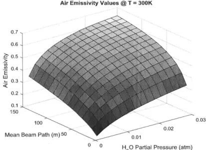
air. In the previous version of UWG, the air emissivity (Ecan) was calculated as shown below:

Ecan = 0.683(1 - exp -1.17X-)' ₍₆₎

which was determined to be applicable mainly for hot gas in an enclosure, such as combustion chamber where the temperature of the gas is much higher than the surface, and where the process is usually accompanied by emission of light (flame). Using this formulation, the emissivity values of the air were

calculated to be in the range of 0.3~0.5 and also reproduced in Figure 4-5 for a range of mean beam

Air Emissivity Values @ T = 300K 0.7 0.6 0.5 LI) 0.4 E uIJ 0.2 150 100 0.03

Mean Beam Path (m) 50 0.01

0 0 H 20 _{Partial Pressure (atm)}

Figure 4-5 Air Emissivity Values per previous version of UWG

The values shown above correspond to a similar range as documented for Singapore. These values are substantially higher than the measured scattering and extinction values of IR in the atmospheric air which show attenuation coefficient due to absorption at less than 1% per km for the IR wavelengths that correspond to the surface temperatures in the range of 300K (Bueno et al., 2014; Fenn et al., 1985; Yates & Taylor, 1960).

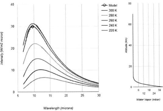
For further validation of the updated assessment on the IR absorptivity in air, an online version of MODTRAN (http://climatemodels.uchicago.edu/rrodtran/) was used to evaluate the IR intensity at high altitude (1km) looking down at the ground surface temperature, as shown in Figure 4-6. The simulation shows that at 1km altitude, the layer of air between the surface and the observation height is mostly transparent to the IR radiation and the attenuation of IR intensity is very low. The plot was generated

with CO2 (ppm) = 400ppm, CH4 =1.7ppm, water vapour scale set to 100% humidity (34mbar), looking

down from 1km altitude, using 1976 U.S. Standard Atmosphere with no cloud or rain, other parameters set to default, and the surface temperature set to 300K. The MODTRAN model used for online

40 7': 30 10 1 10 15 2 30 Model - 300 K 280 K 260 K 240 K -~220 K 13 M0 W4avength (mucrons)

Figure 4-6 IR Transfer Characteristics at 1km height, MODTRAN

These observations show that the previous versions of UWG over-estimated the IR absorption

coefficient of the bodies of air. To correct for this, in the updated model, the bodies of air are essentially transparent to LW emitted from surfaces, as well as downward longwave radiation specified in the EPW file. Other atmospheric radiative transfer models such as Discrete Anisotropic Radiative Transfer (DART) are also validated against MODTRAN (Gastellu-Etchegorry et al., 2015). In addition, the updated model removes the account for IR exchange of energy between the internal surface of the building and the internal air in the building model, as the internal air is considered transparent and the inner surfaces have temperatures sufficiently close to each other with difficult view factors to calculate.

The net IR fluxes for the external surfaces were also updated so that IR radiation flux is calculated directly rather than using linearized coefficients, as the linearization error increases with the

temperature difference between the two surfaces, such as that between the sky and the urban surfaces. The calculations for the net LW heat emission are shown below for the roof, road and the wall surfaces.

roof,I R - eroof (QDownLW - _(o7of

Qroad,LW = eroadVroad-sky(l - rshad)(QDown,LW - UTroad) +

VFroad-wauleroadewaul(1 - rshad)(Twall - Troad), 8

Qwall,LW = eroadVFwall-sky(QDown,LW - UTwall) + VFwal-raoderoadewall(l - rshad)(Troad - Twaii),

where a is the Stephen-Boltzman constant, VFroad-sky is the radiation view factor from road to the sky and VFroad-wali is the view factor from the road to the wall, rshad is the road shaded by trees (assumed to be in radiative equilibrium with its surroundings), and QDownLW is the downward longwave emission from the sky as indicated in the EPW file. The road shading by trees is taken into account only during the specified months when vegetation is available (i.e. for deciduous tree).

The infrared heat flux is calculated for each building's roof and wall surfaces, while the road uses the weighted average of wall temperatures of the buildings.

4.2.5 Humidity

In the updated UWG, the humidity calculation for the canyon was also removed and the rural absolute humidity value is assumed to be the same for the urban area, which is then used to calculate the relative humidity value for the EPW file. This results in a slightly lower relative humidity in the canyon when compared to the rural weather due to the higher temperature in the urban area. On the other hand, the calculation for the moisture content in the air requires consideration of vegetation, soil moisture content, diffusivity of moisture in the air, moisture from combustion and the evaporation from a nearby body of water such as river, lakes and sea which were not modelled, and thus it was difficult to justify a canyon humidity balance based only on the building air and the latent heat from evaporative cooler and vegetation. In addition, the validation for the latent heat balance of the urban canyon was not provided in the previous versions of UWG and the latent heat exchange between the UBL and the UCL, as well as within the VDM was not considered.

Therefore, when the solar radiation is received by the vegetation fraction on the road, only the sensible portion of the energy absorbed is considered in the overall energy balance.

4.2.6 Urban Wind Speed

When the urban weather file is generated, the wind speed indicated in the file is now based on the calculated canyon wind speed, instead of the rural weather station wind speed as previously output by the previous version of UWG. This accounts for the lower wind speed in the urban area due to higher obstacle heights in the urban area, where the canyon wind speed calculation is defined in the Appendix

of 2014 study of urban microclimate in Singapore (Bueno et al., 2014).

4.2.7 Anthropogenic (Traffic) Heat Flux

Per Quah and Roth, in an urban area, the anthropogenic heat sources are assumed to consist of buildings, traffic and humans so that,

Qtotal = QBLD QTraffic + QHurnani (10)

where the anthropogenic heat fluxes range from low of 13W/M2

to 113 W/m2

with building fluxes

consisting of up to 46-82% of the total heat flux (Quah & Roth, 2012). In the UWG, the building term

(QBLD) is accounted by the building energy model that also includes the occupant heat load, and the non-building anthropogenic heat is assumed to consist only of traffic, which peaks at around 15W/m2 for Singapore. While the previous version of UWG assumed constant heat load profile, the updated UWG incorporates a user-specified hourly schedule for weekday, Saturday, and Sunday, an example of which is shown in Figure 4-7.

Traffic Schedule WD ---- Sat -Sun 0.2 0 0 6 12 18 24 HOUR

4.2.8 Soil Temperature and Road Layers

The updated version reads the soil temperature from the EPW file provided, based on each month of the year, at depths of 0.5m, 2m, and 4m and uses these temperature values as the boundary condition for solving the road layer temperature profile, instead of a single ground temperature based on the average temperature of the weather file for the whole year. It is noted that the EPW-provided values are also simulated values using soil diffusivity value indicated in the application EPW file. When the thickness of the road element is less than the soil temperature depths, it is padded with additional soil layers until the nth layer depth is within the indicated soil depth level +/- 2.5cm.

300 295 290 25 S285 E C) 275 270

Ground Temperature Variation by Depth and Month

o.5m --- 40m-- -- -0 2 4 6 Month 8 10 12

Figure 4-8 Ground Temperature Variation

In addition, the road elements are divided into thinner layers with maximum thickness of 5cm, so that

the surface temperature fluctuation can be modelled more accurately.

4.3 URBAN BOUNDARY LAYER MODEL

The UBL model based on the energy balance is the same as the 2012 version of the UWG, defined as:

VUBLPCv = Hurb + f Uref Pcp (Orej - Ourb)dAf, (11)

which removes the IR portion of the energy balance formulation that was added in the 2014 version of

assumed to be negligible when the vertical profile of the potential temperature becomes constant so that only the heat flux from the bottom control surface or the sides drive the energy balance of the UBL. The advective heat flux is driven by either the horizontal flow or by the radial urban-breeze circulation where the direction of the wind is not taken into account, so that the rural temperature data is assumed to be applicable to the large concentric region surrounding the urban area (Hidalgo, Masson, & Gimeno, 2010). The height of the urban boundary layer, set to 1000~1500m during the day and 50-80m during the night, also corresponds to the values found in other LIDAR measurements (Barlow et al., 2011; Menut, Flamant, Pelon, & Flamant, 1999).

Assuming that the canyon air has very little thermal mass, the urban heat flux (Hurb) is defined as the sum of all surface sensible heat fluxes and waste heat as follows:

Hurb ~ Qsensroad + Qtraffic + Qveg + EN=1senswai,i +

Qsens,windowi + Qvent&inyafi + Qwaste,i + Qroof,i),

for N building types simulated.

4.4 BUILDING ENERGY MODEL

The UWG building energy modelling is based on the original UWG work with modifications that include cooling and heating load calculations and the scheduling of the loads as described in this section (Bueno,

Pigeon, Norford, & Zibouche, 2011).

4.4.1 Energy Balance

The internal building energy balance for each building is defined as follows in the calculation of the temperature of the internal air mass, assuming a uniform temperature within the entire building envelope:

dT

VBLDPCV dt1- = Awallhwaiu(Twal - Tair) + AwinUwin(TucI - Tair)

+ Amass hmass (Tmass - _{Tair) + Aroof hroof (Troof - Tair)}

(13)

+

VventPCp

~ingf

where A, h, and T correspond to area, convective coefficient and the temperatures of the elements noted by the subscript (internal temperatures for wall and roof). The internal heat loads correspond to solar heat gain based on the window area, and the internal sensible heat load from light, occupants and electric equipment. Similar to the energy balance of the urban canyon, the model solves for Tai, where

dTair is equal to zero, and solves for each footprint area of the building, so that the temperature is then

dt

bounded by the temperature of the wall, roof, mass, and the canyon air temperature via infiltration and ventilation. The wall, mass (floor & ceiling) and the roof areas are defined per Table 4-2, and the walls do not account for internal walls that divide the building floor space.

The updated UWG treats the sensible, latent, and the radiant heat separately, so that Fsens + Fran +

Flat = 1 for the occupant, equipment, and light component internal heat load sources. The sensible and latent heat portions are added directly to the indoor sensible and latent energy balance, while the radiant heat is added to the ceiling and floor, as summarized in Table 4-3:

Occupant Equipment Light Added to

Sensible Fraction 0.5 0.5 0.3 Air

Radiant Fraction 0.2 0.5 0.7 Mass

Latent Fraction 0.3 0 0 Air

Total 1 1 1

Table 4-3 Sensible, Radiant and Latent Fraction of Heat Loads

This disaggregation is a departure from the original UWG, which only specified the total internal heat load and the corresponding sensible, radiant and latent portion of the internal heat load, to take into account the variation in types of heat load. Internally, the radiant heat from lights and occupants is added to the heat flux received by the mass element of the building, assuming that the view factor from the lights and the occupants to the floor and the ceiling of each floor are close to unity and that the load values are small enough to warrant approximation. The gas equipment is assumed to not contribute to the total internal heat load as it tends to be used in well ventilated areas; on the other hand, similar to space and water heating, a fraction of it is added to the waste heat from the building based on the heating efficiency specified.

4.4.2 DOE Reference Buildings

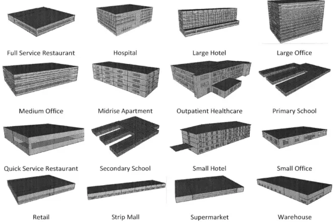
In order to simplify the estimation of UHI effect for various US cities, commercial buildings data were imported from the Department of Energy (DOE) online database, with sixteen different building types, three construction eras (pre-80s construction, post-80, new construction) and sixteen different climate zones, representing a total of 768 different building archetypes generated from the Commercial Building Energy Consumption Survey (CBECS) (Kneifel, 2012). The energy model takes into account schedules for

lighting, electrical plugged-in equipment, occupancy and gas equipment (if available). The reference building types are shown in Figure 4-9 below.

Full Service Restaurant

Medium Office Hospital Midrise Apartment Large Hotel Outpatient Healthcare Large Office Primary School

Quick Service Restaurant

Retail

Secondary School

Strip Mall

Figure 4-9 DOE Reference Commercial Building Types

Each building has three built-eras where the major difference is the wall insulation, window U factor, and lighting electricity consumption, while the physical sizing of the building and zone area remain the same. In order to model the building energy consumption using the UWG, the buildings were simplified

0

Small Hotel

Supermarket

Small Office

to contain only one zone, and the weighted average was used to calculate the internal heat load from each zone for occupancy, lighting and electrical equipment. An example is shown in Table 4-4 below for the 'Full Service Restaurant' building type.

Conditioned Zone Area Lights Elec Equip Gas Equip Hot Water

(m 2) (W/m2_{) (W/m}2

) (W/m2) (L/h)

Dining 372 266.77 27.39 60.28

Kitchen 139 7.50 16.38 376.74 1198.34 503

Total 511.2 196.06 24.39 146.59 326.83 503

Table 4-4 Full Service Restaurant Averaged Heat Load

Assuming that zones where gas equipment is used are well-ventilated (indicated by exhaust rate for EnergyPlus models), the gas equpment heat loads are not included in the internal sensible heat load. On the other hand, the waste heat to the urban canyon, similar to heating, is considered for both service hot water and gas equipment.

Hot water consumption is modelled based on the DOE reference model of water consumption schedule, set at the service water temperature of 49C (which is the water supply temperature specified by EnergyPlus schedule for the usage of most buildings). The ground temperature at 2.Om provided in the EPW weather file is used as the cold water inlet temperature. All water heaters are assumed to be

powered by gas, so that the efficiency of heating water is the same as gas heater space-heating

efficiency, typically at around 0.8. Similar to gas equipment, the hot water usage does not contribute to the building internal load but is assumed to drain away after use, and the energy consumed for heating water is calculated as:

QSWH = rnSWHCp,H20 (TSWH - Tcold)/egas, (14)

for each floor area of the building with the mass flow rate for hot water specified by the building schedule.

The space-heating rate is determined by setting the Tair in Eq. ( 13 ) to the heating temperature set point and determining the heat requirement limited to the maximum heating capacity. In the updated

UWG model, the heating mechanism works as simple internal heat load added to the building control volume based on the heating requirement rather than based on the supply air temperature and mass flow rate, so that other types of heating such as radiators can be simulated. The cooling demand is determined assuming the supply air temperature fixed at 10'C and assumed to be at 90% humidity so that the model then solves for the required mass-flow rate required to achieve the cooling set-temperature for the building. This is slightly different than the building energy models used in the

previous versions of UWG where the mass-flow rate was set as constant based on the cooling capacity and the supply temperature was solved. While both approaches give similar results, the prior approach assumed the same constant mass flow rate whether the building was being cooled or heated and at times lead to excessive supply air temperature fluctuation and was therefore updated.

SchEquip SchLight SchOcc SetCool SetHeat

WD Sat Sun WD Sat Sun WD Sat Sun WD Sat Sun WD Sat Sun

0.1 0.1 0.1 0.1 0.1 0.1 0.25 0.35 0.35 0.25 0.35 0.35 0.35 0.25 0.25 0.25 0.35 0.35 0.35 0.25 0.25 0.25 0.25 0.25 0.1 0.1 0.1 0.1 0.1 0.1 0.25 0.35 0.35 0.25 0.35 0.35 0.35 0.25 0.25 0.25 0.35 0.35 0.35 0.25 0.25 0.25 0.25 0.25 0.1 0.1 0.1 0.1 0.1 0.1 0.25 0.35 0.35 0.25 0.35 0.35 0.35 0.25 0.25 0.25 0.35 0.35 0.35 0.25 0.25 0.25 0.25 0.25 0.45 0.15 0.15 0.15 0.15 0.45 0.9 0.9 0.9 0.9 0.9 0.9 0.9 0.9 0.9 0.9 0.9 0.9 0.9 0.9 0.9 0.9 0.9 0.9 0.45 0.15 0.15 0.15 0.15 0.45 0.9 0.9 0.9 0.9 0.9 0.9 0.9 0.9 0.9 0.9 0.9 0.9 0.9 0.9 0.9 0.9 0.9 0.9 0.45 0.15 0.15 0.15 0.15 0.45 0.9 0.9 0.9 0.9 0.9 0.9 0.9 0.9 0.9 0.9 0.9 0.9 0.9 0.9 0.9 0.9 0.9 0.9 0.05 0 0 0 0 0.05 0.1 0.4 0.4 0.4 0.2 0.5 0.8 0.7 0.4 0.2 0.25 0.5 0.8 0.8 0.8 0.5 0.35 0.2 0.05 0 0 0 0 0 0.05 0.5 0.5 0.4 0.2 0.45 0.5 0.5 0.35 0.3 0.3 0.3 0.7 0.9 0.7 0.65 0.55 0.35 0.05 0 0 0 0 0 0.05 0.5 0.5 0.2 0.2 0.3 0.5 0.5 0.3 0.2 0.25 0.35 0.55 0.65 0.7 0.35 0.2 0.2 24 30 30 30 30 24 24 24 24 24 24 24 24 24 24 24 24 24 24 24 24 24 24 24 24 30 30 30 30 24 24 24 24 24 24 24 24 24 24 24 24 24 24 24 24 24 24 24 24 30 30 30 30 24 24 24 24 24 24 24 24 24 24 24 24 24 24 24 24 24 24 24 21 15.6 15.6 15.6 15.6 21 21 21 21 21 21 21 21 21 21 21 21 21 21 21 21 21 21 21 21 15.6 15.6 15.6 15.6 21 21 21 21 21 21 21 21 21 21 21 21 21 21 21 21 21 21 21 21 15.6 15.6 15.6 15.6 21 21 21 21 21 21 21 21 21 21 21 21 21 21 21 21 21 21 21 SchGas SchSWH

WD Sat Sun WD Sat Sun

0.02 0.02 0.02 0.02 0.02 0.05 0.1 0.15 0.2 0.15 0.25 0.25 0.25 0.2 0.15 0.2 0.3 0.3 0.3 0.2 0.2 0.15 0.1 0.05 0.02 0.02 0.02 0.02 0.02 0.05 0.1 0.15 0.2 0.15 0.25 0.25 0.25 0.2 0.15 0.2 0.3 0.3 0.3 0.2 0.2 0.15 0.1 0.05 0.02 0.02 0.02 0.02 0.02 0.05 0.1 0.15 0.2 0.15 0.25 0.25 0.25 0.2 0.15 0.2 0.3 0.3 0.3 0.2 0.2 0.15 0.1 0.05 0.2 0 0 0 0 0 0.15 0.6 0.55 0.45 0.4 0.45 0.4 0.35 0.3 0.3 0.3 0.4 0.55 0.6 0.5 0.55 0.45 0.25 0.2 0.25 0 0 0 0 0 0 0 0 0 0 0.15 0.15 0.15 0.15 0.15 0.15 0.5 0.15 0.45 0.5 0.5 0.5 0.5 0.4 0.45 0.4 0.4 0.3 0.4 0.3 0.35 0.3 0.4 0.4 0.55 0.5 0.55 0.5 0.5 0.4 0.55 0.5 0.4 0.4 0.3 0.2

Table 4-5 Simplified DOE Reference Building Schedule (Full Service Restaurant) Hr 1 2 3 4 5 6 7 8 9 10 11 12 13 14 15 16 17 18 19 20 21 22 23 24

A set of schedule is defined for each building type regardless of the climate zone and the built era. An example of the schedule is shown in Table 4-5 for BLD1, Full Service Restaurant, set for each hour of the day and weekday, Saturday and Sunday. The schedules are considered to be applicable throughout the year. For primary school and secondary school building types, there are two sets of schedules

representing the school months and the summer off-months, but only the school-month schedule is used in the simulation as the fraction of school building in the total urban area

to be small.

building stock is assumed

The internal heat load is then calculated using the peak load specified for each building type. The peak loads for six building types are shown below in Table 4-6.

Built No. People Lights Elec Gas SWH Vent Infil

Building Type Period Floors Area (ml) (Total) (W/m2

) uip uip (L/h) (L/s/m2) (ACH)

BLD1: Full Pre8O 1 511.2 196.06 24.39 146.59 326.83 503.5 5.34 2.06 Service Pst80 1 511.2 196.06 24.39 146.59 326.83 503.5 5.34 2.06 Restaurant New 1 511.2 196.06 19.96 146.59 326.83 503.5 5.34 0.55 Pre80 5 22,422 1291.2 21.9 17.4 12.6 1037.2 1.8 0.2 BLD2: Pst8O 5 22,422 1291.2 21.9 17.4 12.6 1037.2 1.8 0.2 Hospital New 5 22,422 1291.2 12.1 17.4 12.6 1037.2 1.8 0.1 Pre8O 6 11,345 1,411 16.51 17.08 18.38 15,230 1.26 0.50 BLD3 Large Pst80 6 11,345 1,411 16.51 17.08 18.38 15,230 1.26 0.50 New 6 11,345 1,411 10.77 17.08 18.38 15,230 1.26 0.13 Pre80 12 46,320 2,397 15.5 10.8 0.0 968 0.5 0.8 BLD4: Large Pst8O 12 46,320 2,397 15.5 10.8 0.0 968 0.5 0.8 Office New 12 46,320 2,397 10.8 10.8 0.0 968 0.5 0.2 BLD5: Pre80 3 4,982 268 16.9 10.8 0.0 112.4 0.5 1.9 Medium Pst80 3 4,982 268 16.9 10.8 0.0 112.4 0.5 1.9 Office New 3 4,982 268 10.8 10.8 0.0 112.4 0.5 0.5 Pre80 4 3,135 80 4.98 5.06 0.0 408.3 0.45 0.69 BLD6: Midrise Pst8O 4 3,135 80 4.98 5.06 0.0 408.3 0.45 0.69 Apartment New 4 3,135 80 4.22 5.06 0.0 408.3 0.45 0.18

Table 4-6 Building Types and Summary - BLD1-6

The hot water peak is specified for the entire building, and ventilation and infiltration rate is assumed to be constant throughout the day.

4.4.3 DOE Building Element Sizing

The thermal conductivity and the volumetric heat capacity of the roof, wall, and the mass layer of the building were determined using the location summary and the R-value of the element, as shown for

BLD2 (Hospital), Pre-1980 construction for four climate zones in Table 4-7. The thickness of the insulation is calculated using the total R-value of the structure and the R-values of the layers that

constitute the structure, such as 1" of stucco, 8" of conrete, and Y2" of gypsum for the type 'MassWall'.

The same climate zone characteristic also specifies the maximum heating and cooling capacity, COP of the HVAC system, and the solar heat gain coefficient (SHGC) and window U-factors.

Miami Houston Phoenix Atlanta

ASHRAE 90.1-2004 Climate Zone 1A 2A 2B 3A

Wall Construction Type MassWall MassWall MassWall MassWall

Wall R-value (m2-K / W) 0.77 0.77 0.77 0.78

Roof Construction Type lEAD lEAD lEAD lEAD

Roof R-value (m2.K /W) 1.76 1.76 1.76 1.76 U-Factor (W / m2 -K) 5.84 5.84 5.84 5.84 SHGC 0.54 0.54 0.54 0.54 HVAC Size (kW) 3,415.76 3,397.93 3,123.55 3,196.82 Heater Size (kW) 3,494.71 3,682.05 3,665.56 3,703.94

Air Conditioning (COP) 5.540 5.540 5.540 5.540

Heating Efficiency (%) 0.79 0.79 0.79 0.79

Table 4-7 Roof, Wall Characteristics for BLD Type 2 (Hospital)

If the calculated insulation thickness is less than 1cm, the structural element is modelled without the

insulation material to avoid excessively thin element layer that may lead to solver instability. Such thin layer of insulation will not affect the overall R-value of the structure significantly and the thermal mass of the insulation will be much smaller when compared to other materials such as concrete and brick. Similarly, other thin layers such as roof-membrane and metal decking are not used for calculations, taking only the surface optical surface properties (albedo and emissivity) into account.

4.4.4 Building Waste Heat

The waste heat to the canyon is based on the HVAC building energy consumption, as well as heating and

hot water usage. While the previous version of the model considered the waste heat based on the total

building energy consumption (Qwaste = Qcons + Qcooling demand), the updated model does not

explicitly calculate the waste heat that includes the building energy consumption; the energy consumed

by light and equipment is added as heat energy to either internal building air mass or the surface, and

waste heat (from condensor for cooling, or from heating efficiency less than one for heating), as well as waste heat from heating water and gas consumption, as shown below:

Qlwaste Qwaste,HVAC + Qwaste,S'H Qwastegas, (15)

I

4.5

The rural station model incorporates the VDM that solves the vertical potential temperature profile based on the ground surface temperature as indicated by the rural weather station data (Bueno et al., 2013). The VDM model remains unchanged from the previous version of the UWG, solving for the vertical potential temperature profile based on the ground air temperature specified by the rural weather station, the sensible heat flux at this node, and using the boundary condition where the change in vertical temperature profile becomes zero at a certain height (zref = 150m). An example of the vertical temperature profile throughout the day is shown in Figure 4-10.

0

Vertical Diffusion Model Profile

299-2989

~'297

Figure 4-10 Example of the Vertical Diffusion Model Temperature Profile

4.6 THE UWG PROGRAM

The UWG is an urban microclimate simulator written in Matlab that uses the rural weather data and the model definition as discussed above to generate the urban weather data, with the program workflow

shown in Figure 4-11. The urban weather output data include an updated dry-bulb temperature (Tdb),

dew-point temperature (Tdp), relative humidity, and wind speed, with the dry-bulb temperature and wind speed as two key system outputs. By providing weather data which are closer to the actual neighbourhood that a new building will be built in, the urban planner can better size the HVAC equipment and estimate the outdoor thermal comfort.

Rural Weather Data

Urban

.-. Microctimate Urban Weather Data

Simulation

Urban Building Configuration

Figure 4-11 Urban Microclimate Workflow

Further details of the program interface are included in Appendix A. A new Excel interface is developed to ease the specification of modelling parameters when executing the UWG program, where the user can specify both the rural weather data file to be used and the urban building configuration, including the building types to be used. The macro-enabled Excel file works with a compiled version of the UWG as a standalone urban microclimate simulation package.

In addition to the changes described in the previous sections, other minor changes to the program include the simplification of the XML interface code and the module structures. The model also checks and divides up thicker layers into thinner layers of specified maximum thickness (currently set at 0.05m). The changes to the model that had incorporated multiple areas were removed, as the

multi-neighbourhood effect was not deemed to be substantial (Bueno et al., 2014). The auto-sizing function that determines the capacity of the cooling was removed and the program assumes that the

cooling/heating system is sufficient to meet the building cooling/demand as needed. The previous version determined the HVAC capacity as 120% of the peak cooling demand between July 15 and20, so that the demand of the hottest days of the year is met. For the new UWG, when the auto-sizing is specified (when the building is specified without peak cooling/heating capacity) the UWG assumes unlimited HVAC and heating capacity so that the target cooling/heating temperature is always met. The main files for the UWG program are listed below in Table 4-8.

Main Files

RunUWG. :I sm Main user interface file (new)

UWGv4 .0 .e:<e The executable file. Requires Matlab RunTime v9.0 (32-bit) to run. The current executable version is compiled with Matlab R2015b.

Main Matlab Files

UWG. m Main Matlab function file.

Building. m Defines the building class type. Contains building energy model for calculating internal

building heat flux. (updated)

InfraCalcs .m Calculates the infrared radiative exchange between external surfaces (road, wall, roof), and

also with sky. (updated)

UCMDe f .it Defines the UCL class type and contains the UCL energy model. (updated)

UBLle f .m Defines the UBL class type and contains the UBL energy model. (updated)

So!ar Calc s .m Calculates the solar radiation on roof, wall, and road surfaces, based on the TEM scheme, including the GMT hour correction.

RSMDe f .mt Defines the rural vertical diffusion model (VDM).

Element .m Defines the element (wall, road, roof, and mass) classes and includes functions for

calculating layer temperatures.

Misc. Files

readDOE .m Reads DOE summary Excel files (16) each of which contain zone data schedule for three

readEP. mi

UWGdata .mat

different periods. Generates building class types needed for UWG. Required only when DOE

class types have been modified, and a new Ref DOE .mat file will be generated.

Reads the building energy data file (Excel) from Energy Plus run and plots building energy consumption data.

Matlab file containing class elements (UCM, UBL, BEM, Weather), for post-simulation analysis.

Table 4-8 Main UWG Program Files

5 CASE STUDY AND MODEL VALIDATION

This chapter discusses results of the simulation runs, which include comparison with the results against experimental data from previous UWG studies to ensure that the updated model produces valid results.

5.1 VALIDATION OF URBAN WEATHER

Simulations were run using the available urban parameters from the previous UWG studies from the BUBBLE and CAPITOUL experiments (Bueno et al., 2013) as well as Singapore (Bueno et al., 2014). The main urban parameters used for the simulations are listed in Table 5-1. The structural elements of the DOE mid-rise apartment building based on Chicago (for BUBBLE/CAPITOUL) and Miami (for Singapore) climates were modified according to the building descriptions in the two studies mentioned.

Daytime UBL Height Nighttime UBL Height

Ave. Building Height Building Density

Vertical to Horizontal Ratio

Urban Vegetation Fraction

Road Albedo

DOE Building Type used

Cooling System Traffic Heat (max)

Waste Heat Fraction to Canyon Exchange Coefficient

Rural Station, if known

Rural Vegetation Fraction

Temperature Reference Height

BUBBLE 1000m 50m 14.6m 0.54 0.48 0.16 0.08 Mid-rise Apartment (Zone 5A (Chicago), post-80s build, wall albedo = 0.25) No 20W/M2 1 1 0.8 2.6m (urban) 1.5m (rural) CAPITOUL 1000m 50m 20m 0.68 1.10 0.08 0.08 Mid-rise Apartment (Zone 5A (Chicago), post-80s build, wall albedo = 0.25) No 20W/m2l 1 1 0.8 19m (urban) 2m (rural) SINGAPORE (Punggol) 700m 80m 26m 0.38 1.55 0.19 0.1 Mid-rise Apartment (Zone 1A (Miami), post-80s build, wall albedo = 0.15) Yes (40%) 10W/m2 0.4 1 Selatar 0.8 Unknown

Table 5-1 Main Parameters for BUBBLE, CAPITOUL and Singapore Simulations

The schedule and the internal heat loads defined by the DOE reference building were used for all cases;

air-conditioning, the current study assumes all of the building stock to use air-conditioning but only 40% of the HVAC waste heat is added to the canyon air.

5.1.1 Comparison: BUBBLE

Figure 5-1 shows the comparison of the results between the two versions of UWG, with the hourly data

averaged over the period of observation (June 10th to July 10th) for Basel, Switzerland. The left plot,

taken from the UWG study from 2012 (Bueno et al., 2013), is compared against the new version of UWG on the right. The UHI pattern of warmer city temperature from late afternoon to early morning and slightly cooler urban temperature is observed in both plots.

A5 3S --- TRUR -T_UCL 30 - - 30 20 (4MM OIW1) I

~

Figure 5-1 BUBBLE Comparison: Bueno (2013) (left) vs. new UWG (right)

The updated UWG results are similar to the previous version, showing slightly cooler temperature than the observed temperatures.

5.1.2 Comparison: CAPITOUL

Similar to the BUBBLE experiment, the new UWG compares well against the CAPITOUL data for the months of July (top), October (middle) and January (bottom) shown in Figure 5-2.

... ... .. ... ... (W --' IO " A)0 - _RU - TUCL 30 10 0 4 8 12 16 20 24 HOUR 30 ---... - --- - TRUR - ---TUCL 20 -l --- -10 0 (4W 10X ) 02 1 t( 24' Wi 8 12 16 HOUR 20 24 20 -- T RUR T_UCL 15 0 -. -....- --...-.-... 0 4 8 12 16 HOUR 20 24

Figure 5-2 CAPITOUL Comparison: Buena (2013) (left) vs. new UWG (right) - Jul/Oct/Jan

5.1.3 Comparison: Singapore

The Singapore simulation was also repeated, with the results of February (top) and July (bottom) shown in Figure 5-3 below. The observational data from the previous study in February shows a rather unusual UHI behaviour where the average urban temperature stays below the average rural temperature until about 6pm. The updated UWG urban temperature simulation is similar to the previous UWG prediction and deviates from the observation by predicting warmer temperatures than observed.

I

TTT'~Z

F-L

---L

1

1~

-

-

1

Figure 5-3 Singapore Comparison: Buena (2014) on left vs. new UWG on right

Nonetheless, the new UWG result shows better agreement with the observation for the July simulation where the previous version seems to have under-predicted the urban temperature during the night period.

5.1.4 Observations

The updated UWG shows good agreement with the previous version of the UWG. While quantitative validation is not feasible due to the lack of numerical data from earlier studies, the plots show that the updated urban microclimate model behaves in an expected way and produces results that are similar to the previous version.

The diurnal pattern of UHI is consistent in all simulations, with the urban area being slightly cooler than the rural area in the late morning from about 8am to 12pm and being warmer from early afternoon to early morning the next day. The BUBBLE and CAPITOUL experiments show that this agrees with the actual UHI effects, although this trend is not observed in the February data from Singapore. However, without access to the actual field data, it is not possible to further investigate behaviour.

-T RUR TUCL 0 4 8 12 16 20 24 HOUR -- TRUR TUCL 0 4 8 12 16 20 24 HOUR