Continuous-spin Ising ferromagnets.

CONTINUOUS-SPIN ISING FERROMAGNETS by

GARRETT SMITH SYLVESTER': B. S. E., Princeton University

1971

SUBMITTED IN PARTIAL FULFILLMENT

OF THE REQUIREMENTS FOR THE

DEGREE OF DOCTOR OF

PHILOSOPHY at the

MASSACHUSETTS INSTITUTE OF

TECHNOLOGY February, 1976

Signature of Author .

...

••...

,- Department c( Matheatics Certified by .- ... e ...

.']hesi§ Sup soAsol, ,

Accepted by...

Chairman, Departmental Committee

" Supported in part by the National Science Foundation under Grants MPS 75-20638 and MPS 75-21212.

Archives

MAR 9

1976

JuRAS!t

2

ABSTRACT of

CONTINUOUS-SPIN ISING FERROMAGNETS by

GARRETT SMITH SYLVESTER

Submitted to the Department of Mathematics on January 14, 1976 in partial fulfillment of the requirements for the degree of

Doctor of Philosophy

We define and analyze the Gibbs measures of continuous-spin ferromagnetic Ising models. We obtain many inequalities inter-relating the moments (spin expectations) of these measures. We investigate the dependence on temperature and magnetic field parameters, and find that at low temperature the first moment of the Gibbs measure (the magnetization) is discontinuous in the magnetic field parameter for all nontrivial models in two or more dimensions. _{Thus the appearance of a phase transition is generic:} all nontrivial continuous-spin ferromagnets in at least two dimen-sions become spontaneously magnetized at sufficiently low temperature.

Thesis Supervisor: Arthur M. Jaffe Title: Professor of Physics

TABLE OF CONTENTS

page

Chapter I: Introduction 5

Chapter II: Inequalities 12

II.1: Introduction 12

11.2: Inequalities by Duplicate Variables 14

11.3: Discussion 24

11.4: Change of Single-Spin Measure 31

Chapter III: Gaussian Inequalities 37

III.1: Introduction 37

111.2: Proof of Gaussian Inequality 39

Chapter IV: Ursell Functions 44

IV.1: Introduction 44

IV.2: Representations of Ursell Functions 48 IV.3: Signs of Ursell Functions for Ising Ferromagnets 51

IV.4: Miscellaneous Results 59

Technical Appendix: Proof of Lemma IV.3.2 67

Chapter V: Infinite Ising Models 72

V.1: Introduction 72

V.2: The Infinite-Volume Limit 75

V.3: Clustering, Correlation Length, and Long-Range Order 89

V.4: Spontaneous Magnetization 111

V.5: Phase Separation and Breakdown of Translation Symmetry 119 V.6: Applications to Quantum Field Theory 126

TABLE OF CONTENTS (cont'd)

page Chapter VI: Unsolved Problems and Concluding Remarks 130

Acknowledgements 136

Appendix A: Extensions of Theorem 11.2.6 137

Appendix B: Computational Algorithms for Ursell Functions 144

Appendix C: Transfer Matrices 156

Chapter I: Introduction

In this thesis we investigate continuous-spin ferromagnetic Ising models, with principal emphasis on the inequalities they obey and

the remarkable low-temperature phenomena they exhibit. Mathematically, the study of these models amounts to the analysis of a physically-motivated class of probability measures, called Gibbs measures, carried

on finite or infinite-dimensional product spaces

i.he

models we

consider, which are rigorously defined at the close of the introduction, generalize the original notion of Ising and Lenz [1I] in two ways:

the spin variables 0r may assume any real values with some a priori probability measure-V instead of. merely assuming the values

+1, and the energy of a configuration of spins may include many-body terms instead of only two-body terms. Physically, continuous-spin ferromagnets are of interest not so much because they resemble real

crystals - with our degree of generality this resemblance is tenuous - but rather because they accurately approximate Euclidean scalar quantum fields

[431 and so provide a simpler structure for developing conjectures and proving theorems that carry over in the limit to the more difficult models of

quantum field theory. Mathematically, continuous-spin ferromagnets are of greatest interest for the striking dependence of the moments of the Gibbs measure on certain parameters representing physical variables such as

temperature and magnetic field strength. One generally expects that the limit of a naturally-arising convergent sequence of continuous functions is

continuous. By contrast, one of the main theorems in this thesis is a proof of precisely the opposite: certain moments of the Gibbs measure, which are

are necessarily discontinuous.

We now give a synopsis of our results. Chapters II-IV deal with inequalities for finite Ising ferromagnets, whose Gibbs measures are defined on finite products TiR. In Chapter II we introduce the convenient method of

duplicate variables, and use it to give a simple, unified derivation for continuous-spin ferromagnets of inequalities proved by other methods

in various special cases by Griffiths

[17],

Griffiths, Hurst, and Sherman

[Ih],

Ginibre [1Z], Lebowitz [ZB] Percus (39•, and Ellis and Monroe C8 ]. With a different technique, we derive an inequality for change of single-spin

measure which will be very useful in our subsequent analysis of low-temperature phenomena. While some inequalities of this chapter hold for all continuous-spin Ising ferromagnets, others are restricted in their domain of validity. Chapter III invokes combinatoric techniques to give a new simplified

proof of a Gaussian-type inequality discovered in its present form by Newman (36j. In Chapter IV, we combine the method of duplicate variables with additional combinatoric techniques to investigate the signs of the Ursell functions u_{n ( generalized cumulants of the Gibbs measure) of spin-½} finite ferromagnetic Ising models. We represent these cumulants as moments of a measure on a larger space, and use this representation to prove

complete results through order n=6. A reduction formula then gives partial results for higher orders. We present formulas for the Maclaurin coefficients of (functions closely related to) the Ursell functions when n<8. Our methods yield additional inequalities, though we have no application for them

at present. In a related appendix (Appendix B) we describe a computational algorithm for the evaluation of (functions closely related to) Ursell

functions of all orders, and the results of a computer study using it.

Chapters II-IV include, with one exception, proofs of all major inequalities for finite ferromagnetic Ising models of which the author is aware. This exception is the F.K.G. inequality [ 11 ], which we shall only use at one point in Chapter V. Although our interest lies in models with real-valued spins, in some cases our results extend to models with vector-valued spins, and where possible we try to point this out.

With the inequalities of Chapters II-IV serving as the primary investigative tools, we turn in Chapter V to the study of infinite continuous-spin

Ising ferromagnets. After making some preliminary definitions, we construct the infinite-volume limit Gibbs measure for a very large class of models by using C*-algebraic techniques, and we give an easy proof that it has finite moments in many cases of interest. With these fundamental results

established, we undertake an analysis of three closely-related low-temperature cooperative phenomena: long-range order, spontaneous magnetization, and

phase separation. We begin with a discussion of the decay of spin correlations when the separation of two clusters of spins becomes large. For many models, we show that these correlations must decay to zero for almost all values of a parameter h representing the influence of an external magnetic field, and in some instances this set of potential exceptional points actually reduces further to the single point h=O. In fact, as we next prove, if h=O and the parameter representing temperature is sufficiently low, then

(nontrivial nearest-neighbor ) models in two or more dimensions do have all their correlations bounded away from zero: they are long-range ordered. This is one of our main theorems. To coordinate our results

(for nearest-neighbor models), and characterize the cluster properties of an Ising ferromagnet in terms of spectral properties of its transfer matrix. We next consider the phenomenon of spontaneous magnetization

(discontinuity of the moments of the Gibbs measure in the external field h), and show that it is a consequence of the long-range order previously

established at low temperature. For certain models we combine inequalities of the previous chapter with an explicit computation by Onsager 1[3) to estimate the critical temperature; that is, the temperature for the onset

of spontaneous magnetization. We establish the third cooperative phenomenon, phase separation, as a consequence (in three or more dimensions) of spontaneous magnetization. The final section of Chapter V treats some of the many

applications to quantum field theory of the inequalities derived in Chapters II-IV.

In Chapter VI we present some unsolved problems, and make concluding remarks.

Let us now give some definitions of terms used in the remainder of this thesis, and some physical motivation for them. A finite continuous-spin

ferromagnetic Ising model is a triple

(A.,H,),

where:

(1) The set of sites- is a finite set. We associate with each site

iGS a spin variable cEje, and the product

WIR

is called the configuration space.

(2) The Hamiltonian H is a polynomial on the configuration space with negative coefficients. We write

H

(Y-)=

-

(1)

where the numbers JK are called couplings (or bonds),

4(A)

is the set of finite families ("sets" with repeated elements) in.A , and

qK-is by definition the product

orK=IT

0o

(The distinction between sets and families is not important for our purposes, and we shall largely ignore it.)

(3) _{The single-spin measure 7 is an even Borel probability measure} onjR which decays sufficiently rapidly that if d is the degree of the polynomial H, then

p(alddp(c

co

V

aQGR.

(2)

The linear term -2: q in H is usually thought of as describing the effect of an external magnetic field, while higher-order terms are considered to arise from the mutual interaction of the spins. We usually recognize this distinction by writing

_~

_{in the Hamiltonian instead of -i Ji .} A pair interaction is a Hamiltonian of degree two. In connection with the decay condition (2) on the single-spin measure we define for d,0

114

Even

loreI

d pe'o661

-7

vIe

1Xý(jlj)diV()<cax.

VteJ1R3

(3)

and set

nl

174

₍₄₎

A model (.,H,-v)is called connected if any pair of sites i,jGjA is connected by a finite chain K , K2,''',K ef) with JK '",* ,J'4 0, iEKI, jEK,, and V

The Gibbs measure I of ( ,H,-) is the measure on the configuration space tk=jT1 defined by

S=E

e1(_M))1T

A

( EclR measurable; (5)

here

•o)

i•s

is

a

_{parameter representing inverse temperature. Note that}

this measure favors lower values of H. The normalization factor in (5) is called the partition function and traditionally denoted by Z:

s1

4expIN(

iV0" .(6)

We indicate (thermal) expectations with respect to the Gibbs measure at

inverse temperature P by angular brackets

< Hy,)P>

,

omitting the descriptive

arguments H,) when they are clear from context:

<j;Hv

1

3>z

<f>4i

=

(7) Physically, the sites . may be thought of as atoms in a crystal, and

the spin variable oj at each site 16A as a classical version of the quantum-mechanical spin each atom possesses. The single-spin measure describes

the spin probability distribution of a completely isolated atom. A point 0' in the configuration space corresponds to a state of the system, and H(0') is the energy of that state. Note that the ferromagnetic condition JK0O causes configurations in which all spins 0_{j have the same sign to}

have generally lower (more negative) energies. If we allow the crystal

to exchange energy (but not mass) with a large heat bath at temperature - , it will reach eventual equilibrium. According to the principles of statistical mechanics, the probability of finding the equilibrium system in some subset Ec¢]'- of the configuration space is given by the Gibbs measure (E).A

We conclude the introduction by describing our notational conventions. Chapters are given Roman numerals I, II, etc., while sections within a

chapter have Arabic numerals 1,2, etc. We use the standard decimal notation to show in which chapter a section appears. Thus, Section 11.3 is the

third section of the second chapter. Important formulas are enumerated sequentially within a section, the numbering beginning again

when a new section starts. As before, we use the standard decimal convention, so that formula (IV.2.12) is the twelfth enumerated formula of the second section in the fourth chapter. Lemmas, propositions, theorems, and corollaries are similarly numbered within a section. If descriptive arguments of a

11

section, formula, lemma, proposition, etc. are omitted in some reference, by convention they are taken to be the values in effect at the point of

the reference. Thus, if in Section IV.4 we see a reference to Theorem 3.1, this means Theorem IV.3.1. References to the numbered bibliography are indicated by square brackets C ].

Chapter II: Inequalities Section 1: Introduction

In this chapter, taken largely from[ 6 ] , we exploit the method of duplicate variables to give a simple unified derivation of continuous-spin Ising ferromagnet inequalities established in various special cases

by Griffiths

11•,

Griffiths, Hurst, and Sherman

[

V1

1,

Ginibre

[ IZ

1,

Lebowitz I[

83,

Percus [

3

1,

and Ellis and Monroe

1

8

1,

obtaining them for

a large class of single-spin measures. The single-spin measure and the Hamiltonian for which the inequalities may be proved become more restricted as the inequality becomes more complex. However, all inequalities hold for a model with ferromagnetic pair interactions, positive (nonuniform) external field, and single-spin measure either - 4+2 40, (spin-) or exp(-P(-r))dc , where P is an even polynomial all of whose coefficients must be positive except the quadratic, which is arbitrary. (Recent work by Ellis and Newman[ 1] elegantly relaxes this condition on P: it need only be an even continuously differentiable function whose derivative

is convex on Od) .) The Percus inequality is akin to the Fortuin-Kasteleyn-Ginibre inequality

[111

in that it holds for arbitrary external field,

though the Hamiltonian is restricted to pair interactions. We exhibit

interrelationships among these inequalities, deriving the Lebowitz correlation inequality from the Ellis-Monroe inequality in the same way the second

Griffiths inequality may be derived from the Ginibre inequality. The G.H.S. inequality for concavity of magnetization is a corollary of the Lebowitz correlation inequality, as is an inequality which at zero external field shows the fourth Ursell function u4 is negative. These basic results

in the hypotheses of the theorems proved in Section 2 and mention various generalizations. The final section is devoted to an inequality for change of single-spin measure, which will be useful in our later analysis of low-temperature cooperative phenomena. Combining this inequality with a result of Griffiths [\81, we compare the spin expectations of a continuous-spin ferromagnet whose single-spin measure is absolutely

continuous near zero with those of a related model having the same Hamiltonian, whose single-spin measure is concentrated at just two points.

Applications of the inequalities proved in this chapter are given in Chapter V.

Section 11.2: Inequalities by Duplicate Variables

We now state and prove the inequalities for ferromagnetic Ising models

mentioned in Section 1. The proofs employ the method of duplicate variables.

Consider a finite ferromagnetic Ising model (AI,H,V ). (See the final

part of Chapter 1 for notation and definitions.) It is convenient to take

2=

1>)..., N3

so that the spin variables are

y,

2I,"',.-N . Construct the doubled system

(LVA,HH,v ), where AVJ~ is the disjoint union of two copies of J ,

the 2N spin variables are O1),i,. I -N,2 , ) i ... )N , and the Hamiltonian HeH is H(oi,OQz>, O N) + H('r1T2>;,r). Thus, the doubled system consists

of two copies of the original system that don't interact with each other.

Define the transformed variables

Construct also a redoubled system (H

V.Y.VAV,

H H$H( H, 7 ) consisting

of four non-interacting copies of the original, with spins IO>, . ,N

/" It* / ) / ',1 , , and Hamiltonian H(j) , , 0 ) +

H(TZ,, 'N ) + H(dj•,e, ) + H(t',,)"14). As before, define

Now set

Note the reversal of primes between 0(, and ,6

Theorem 1: (First Griffiths Inequality) Let A

G'o.)be

a family of sites in a finite ferromagnetic Ising model

(A

,H,'v) with Hamiltonian

[=-Z

7-

J(

JTo

and arbitrary (symmetric) single-spin measure TA.Then

<01

O.

(4)

Theorem 2: (Ginibre Inequality) Let A,BCo₀(l)be families of sites in a finite ferromagnetic Ising model with Hamiltonian

and arbitrary (symmetric) single-spin measureVE

fJ.

Then

Corollary 3: (Second Griffiths Inequality) Let A,BES(.k) be families of sites in the model of Theorem 2. Then

Theorem 4: (Percus Inequality) Let AE o₀ () be a family of sites in a

finite ferromagnetic Ising model (.• ,,'1V)

with pair Hamiltonian

- -T - i i C

0

and h. arbitrary,

Corollary 5: Let i,j be sites in the model of Theorem 4. Then

Theorem 6: (Ellis-Monroe Inequality) Let A,B,C,DG

Vo(.)

be families of sites in a finite ferromagnetic Ising model (A,H,-7) with pair Hamiltonian

and single-spin measure either discrete and of the form

(spin ), or continuous and of the form

d

(9)

where P is an even polynomial whose leading coefficient is positive, whose quadratic and constant coefficients are arbitrary, and whose remaining coefficients are nonnegative. (Situations where coefficients of P other

than the quadratic may be negative are discussed in Appendix A.) Then

Corollary 7: (Lebowitz Correlation Inequality) Let A,BECV o() be families of sites in the model of Theorem 6. Then

Corollary 8: (Griffiths-Hurst-Sherman Inequality) Let i,j,k be sites in the model of Theorem 6. Then

Corollary 9: Let i,j,k,l be sites in the model of Theorem 6. Then

<(7ic·

O,

O<9~>

-LT"j0><Q0>

a _k

- <i

,

+

Z,

(13) The proofs of Theorems 1,2, and 6 all proceed similarly, by reduction to the case of a model with a single site and zero external field. The inverse temperature

P

is inessential and we set it to one. We must show

that a thermal expectation

<f>,

Se

RTJ/dv

/S

e

TdV

is nonnegative. The normalization factor (partition function) in the

denominator is positive, so we ignore it. We first verify that in the trans-formed variables the Hamiltonian is a polynomial with nonpositive coefficients. Expanding exp(-H) in its Taylor series, we obtain a sum with nonnegative

coefficients of integrals of products of the transformed variables against the product of the single-spin measures. Since each integral factors over the sites, it suffices to show that for a single site the integral of any product of the transformed variables is nonnegative; that is, that the theorem holds for one-site models with zero external field. This is what we do. In the proof of Theorem 4 the reduction cannot proceed quite as

far, but essentially the same method prevails. This reduction procedure makes it clear that in all the results of this section we could allow

not commonly studied. Corollary 7 follows from Theorem 6 just as Corollary 3 follows from Theorem 2. Corollary 5 and Corollaries 8,9 are important

special cases of Theorem 4 and Corollary 7.

Proofs:

Theorem 1 (Prf): We want to show

A

K A)JK)

K

(a)dao0

ld

(14)

By expanding the exponential in its Taylor series and factoring the integrals over the sites as described in the previous paragraph, we reduce the

problem to showing

S

J-V (a-)

0

V

.

(15)

By the symmetry of V this vanishes when n is odd, and when n is even the integrand is nonnegative.

QED

Theorem 2 (Prf):

In terms of the transformed variables q and t the Hamiltonian H( ) + H(T) is

JK

)K

+

(

)

(16)

This is a polynomial in the t's and q's with nonpositive coefficients,

because when we expand the product TK(tk-k

)

_{any negative term which}

appears is cancelled by the corresponding term from the expansion of

(t•+c

.

Now by expanding the exponential and factoring the integrals

d(17)

This vanishes by symmetry unless m and n are both even, in which case the integrand is nonnegative.

QED

Theorem 4 (Prf):

The transformation (1) is orthogonal, so in terms of the transformed variables q and t the Hamiltonian H(Oy) + H(r) is

We want to show

C%

exj

('.qZeZ

g(\JItit. 4-

FZdvh(2)'dv(6ir,)t

i t)

₍₁₉₎

By expanding the first exponential exp(( i

•(

q.) we see it suffices to show

>

t

0

(20)

for all possible exponents nk. But this integral vanishes by symmetry unless all the nk are even, in which case the integrand is positive.

Theorem 6(Prf):

The transformation (3) is orthogonal, so in terms of the transformed variables B,(V the Hamiltonian H(6) + H(')) + H(0') + H(Z') is

Since this is

a polynomial with nonpositive coefficients, by expanding(21)

the exponential and factoring the integrals over the sites we reduce the problem to showing

d-

ir(S

ndvd

o)d0

k)IAIA.

(22)

By symmetry this vanishes unless k, ,m,n all have the same parity. When this parity is even the integrand is nonnegative, so we restrict

our further attention to the case of odd parity. At this point we distinguish between discrete and continuous spins.

In the discrete case it suffices to consider spin

½

spins,

-dv(&L)=

t((o

b)

i)

.-

(0--))

d(

(23) for since our transformation of variables is linear the Griffiths "analog system" method [118] may be applied to generate the higher-spin results from the spin

½

case. (The analog system method represents a higher spin by a sum of spin

½

spins in a suitably enlarged model.) Because the exponents k, ,m,n are all odd we may factor out b :

0(

%flc

S =

j

b .

(24)

The first factor is nonnegative since it has even exponents. The second factor is also nonnegative; since

Z

-=2 =C2 = - for spin

½

spins we find

In the continuous case our problem is to show

oi•c

"

eX(-

)

-)-PW

-)

P

C)) d o-

d

t

'j'

>

0

(26)

for odd k,i ,m,n. We claim that when P(cy) +*..+P(PV) is expressed in

terms of

odP3,)

it

has the special form

P(,

Q)

(z,

V

0))

(27)

where Q and R are polynomials with nonnegative coefficients, except

possibly for the coefficients of 20(2 ) ) , in Q. Temporarily accepting this claim, and recalling that transformation (3) is orthogonal, the

integral (26) becomes

-

_A

'

_{[ S'RA"}

_s}

_-

_{( "s•)]}

₍₂₈₎

Replacing o( by-o( and averaging gives

k

i 91

Yin-I'1nj

[cO

'8

siný (4?/ R(o(m..)b9)p(

1

[@]Q(0

)6))Jd(2IS4

8,

(29)

The first factor in (29) is nonnegative since it has even exponents; the

second is nonnegative because R(o( ,,, , ))) 0; the third is obviously

nonnegative.

It remains to verify claim (27). We need only consider the case of a monomial P(X) = X2 p_{. Expanding with the multinomial theorem gives}

4c' 1 (04 8 Y

)

(-a) + 4_{4C]s Q b}

(30)

The coefficient of

d9 g

d _{vanishes unless a,b,c,d all have the same}

parity; it is positive when this parity is even; and, it is negative when the parity is odd. This observation immediately yields claim (27).

Corollary 3 (Prf): We want to show

Using the doubled system we have

CA

><

<BA

><6B-ý>

=

<CoAO-

Oh

Bet8> 4

r(31)

This is the expectation of a polynomial in the q's and t's which may be shown to have nonnegative coefficients just as (16) was shown to have non-positive coefficients. By Theorem 2 this expectation is nonnegative.

QED

Corollary 5 (Prf):

Corollary 5 is a special case of Theorem 4:

0

<(rim,

(32)

Corollary 7 (Prf): We want to show

<Ui tAetB eKav

0

<tAXI

<tA

>0.

Using the redoubled system we have

)z/-K )[

-

(33b)

OX113ý-<tA113ý:<tA g

tA16)=<

(!

A-

B

(33c)

In each case the right-hand side is the expectation of a polynomial in oN) 6 with nonnegative coefficients. By Theorem 6, these expectations are nonnegative.

QED

Corollary 8 (Prf):

As noted by Lebowitz, Corollary 8 is a special case of Corollary 71281:

QED

Corollary 9 (Prf):

Corollary 9 is obtained by symmetrizing the special case

(tt'>-<t1YK~

(35)

Section 11.3: Discussion

In this section we discuss the range of validity of the theorems of Section 2. We indicate generalizations where we can, and illustrate by example the role played by various restrictive hypotheses.

Theorem 2.1 states that for any family of sites A in a suitable model,

(<CA)

o>, O.

(1)

The same proof shows that the spins in the product 0 may be replaced by more general functions. Let

i:IR-)J

~l

be a set of (measurable)

functions such that ,([OP0))c[O)cD) and F.i has definite parity (is either even or odd). Define

F,

=

IT

Then

KFA

)O

.

(2)

Also, note that Theorem 2.1 generalizes easily to ferromagnetic models with vector spins taking values in In , provided that the single-spin measure V is invariant under the n coordinate reflections.

Theorem 2.2 states that for any families of sites A,B in a suitable model,

KAt8»0.

(3)

As remarked by Nelson

1351,

the spins in the product q t may be replaced Ay more general functions. BLet

satisfying the restrictions of the preceding paragraph ( invariance of

[0)~C)

; definite parity) and the additional restriction of monotone increase

on

1[0

) . Define

F

,

iE•

(4)

and if

Ke#

(A)

set

Then

AF<QATý>

z

,

(5)

which has the immediate corollary

We state this as a proposition:

Proposition 1 (Nelson): Let (A.,H,-v) be an Ising ferromagnet with Hamiltonian

and arbitrary (symmetric) single-spin measure

V.

Let

i:A-I1)Eit ,

•.R-~ ,i

be (exponentially bounded measurable) functions

such

that

each Fi,Gi has definite parity, leaves the interval [0) o) invariant,

and is monotone increasing there. Then

This extension of the second Griffiths inequality will be useful in the construction in Chapter V of the infinite-volume limit by virtue of its monotonicity corollary,

Corollary 2: Let (Jt,H,-v) be an Ising ferromagnet with Hamiltonian

_j

'Z

:1 K (rK

₍₈₎

let

.Ack,

and let (~iJr t) be the Ising ferromagnet with Hamiltonian

Hk

(9)

(same JK as in (8); the sum is just restricted to families in(A~f~ ). If

fFi,:•R-ATRi/J

_{is a set of functions obeying the hypothesis of Proposition 1,}

then

K

F<

F(o<);

,ij>

7F'.)H>

(10) In particular,

allA

Ae A')

(11)

Proof: By Proposition 1,

<

F<1

hF('T<Fo.1

-)

o

v

$E

rj().

Thus, if we increase from zero to their final values all coupling constants JK appearing in (8) but not (9),

(•,,•qr)i

\ must increase

to(

Ei)*

H>).

Theorem 2.2 and Corollary 2.3 only have been generalized to vector spin

[26]) dimensions.

Theorem 2.4 and Corollary 2.5 generalize to products of functions of the type for which Theorem 2.2 and Corollary 2.3 are valid. The hypotheses of Theorem 2.4 and Corollary 2.5 are somewhat unusual in that the single-spin measure is arbitrary while the Hamiltonian is restricted to pair interactions. To see that this restriction is valid, note that Corollary 2.5 fails for a spin

½

model with three sites 1i,2,3ý and Hamiltonian

S0-)0

o0-

+

,

o.

(12)

(We find

<

oQ=

Zcr)>

(13)

but

<•),:-i,,ct.

ia•<)

_.

₍₁₄₎

Theorem 2.6 states that if A,B,C,D are families of sites in a suitable model, then

<1A PS'

,(15)

In contrast to the previous results, the same method of proof does not seem to admit a more general class of functions in the product. (For example, it is easy to see that if F:--ýR is any C2 function such that

[F(x,

1

-F(x2)- F(Y

3

)

+

F(X

4

)].[x,-x

1

-x3+

x4]' 0

V

(xt..,X

4

~

which is a key inequality in the proof of Theorem 2.6, then

-that is, F must be of the form already considered.)

The hypothesis of Theorem 2.6 contains restrictions on both the Hamiltonian and the single-spin measure. Example 7.3 of 13 ] shows that the restriction of the Hamiltonian to pair interactions is needed. However, the constraint on the single-spin measure is more severe than necessary. A certain

polynomial R(o(, .,, ,9 ) arises naturally from the single-spin polynomial

P, and for the method of proof to work R(c(2, ,,0 ,9 ) must be nonnegative.

The hypothesis we made ensured this by causing R to have positive coefficients. Clearly, negative coefficients in P, and hence R, are permitted provided

the positive coefficients are large enough to ensure R(o(2, *#, t ) 0.

Restrictions on the coefficients of P were studied from this viewpoint in the appendix of

[46],

reproduced here for convenience as Appendix A. After this work was done, an elegant criterion was obtained by Ellis and

Newman [ J.

They show that Theorem 2.6 and its corollaries hold provided

P is an even continuously differentiable function whose first derivative is convex on 10,0)). Theorem 2.6 is also valid for single-spin measures obtained by limiting procedures from those explicitly permitted. For

example, Lebesgue measure on the interval E-bb6 may be obtained as

the limit

Zu

/Ubi

(6-)d86-=

IOM

earHSAr

. (16)

(Here of course

is

the characteristic function of the

intervalEbb.)

However, some constraint on the single-spin measure is necessary. For example, Corollary 2.9 fails for a one-site model with zero external field having

single-spin measure

S+

o<a<

(17)

since

<o-4>

_3KP2z?

Q

(LL-4i)

(18)

It also fails for a one-site model having single-spin measure exp(-P(a-))da; where

+P~-8"

Z2

1) 4

c ),

ac<

4

(19)

and q is sufficiently large, because as %->o this distribution converges to the preceding one.

Finally, we remark that Theorem 2.6 may be reinterpreted as a theorem about plane rotors. Specifically, we find

Proposition 3: Let A,B,C,DE (J1) be families of sites in a ferromagnetic

plane rotor (A ,H,

7 )with Hamiltonian

=-Z

K I+J(,

J

,3

J

o

(20)

of degree d and single-spin measureV7 on

R2

which is invariant under the two coordinate reflections and is either

(i) concentrated on the unit circle, or (ii) of the form

where P is a polynomial all of whose coefficients are nonnegative, except

for those of (x )2 , ( Y)2 , which are arbitrary. Construct a duplicate

system using primed variables, and define

yi 1 (22)

Then

<O9

vsA

8,

(23)

Corollary 4: Let A,B,C,D be families of sites in the plane rotor of Theorem 3. Then

<' -• - <-> /<(r 0 (24a)

<(Y -\ _<Y

xq>

- > (24b)

<0"0

-<0

><"

o.

(24c)

Section 11.4: Change of Single-Spin Measure

This section, taken mainly from (Z ], is devoted to an inequality for change of single-spin measure. We may view this inequality as a mathematical rendering of the physical notion that the moments of the Gibbs measure (<) decrease when the single-spin measure V7 becomes more concentrated near the origin. By combining the inequality with a result of Griffiths C181, we compare spin expectations of a continuous-spin ferromagnet whose single-continuous-spin measure is absolutely continuous near zero with those of a related model whose single-spin measure is

concentrated at just two points.Chapter V contains an application of the inequality to the study of phase transitions.

Theorem 1: Let (-A,H,V ) be a finite ferromagnetic Ising model, let f be a nonnegative even function monotonically decreasing on [COO) which

is identically 1 on [-CCI) > C 0, and let

AIV

be an even measure supported in [-C,C] which is normalized such that

c=

v+ .v

(1)

is a probability measure:

(aeý + --7)

1T.

(2)

Then the moments of the Gibbs measure decrease when V is replaced by C :

Proof:

measures are permitted to be different at different sites, the replacement of V by -c at a single site causes the spin expectations <A) to decrease. The theorem then follows by successively applying this result to each

site in the model.

Consider a ferromagnet on A with Hamiltonian H and single-spin

measure

'V

at each site iEA. Select a distinguished site lEA, at which we assume the single-spin measure is-V . We want to show

7c

e

hl))

•

O

e-v

)T ,)

(4)

where of course Zc and Z are the partition functions

We rewrite

the expectations in

(4)

to display the dependence on

(5)

We rewrite the expectations in (4) to display the dependence on YV,-V

KOAL;V>'S<

do)

where

<S7~>

er

and

PC

are defined by

-z

I

T,

H()

Ir,=s

T

J-v

(c))

igS-

0

_1:+S

et-1

iZ

0=s

dp-11-'t~~d

~

ts) 5= j T(S) - -1 V (6) (7)

(8)

(9)

D)

S(s)

clpj 7

_.

_(s)=

_jdy-(

₅

₎

_-

(o0)

_(s

₎

(10)

The functions Z(s),( <S and the measures

P

,p have simple interpretations:

the model where the measure -V, at site 1 is [("45)+ . (-S3 , and

p,

pc

are the density measures of the random variable

OI

in

the

models where the single-spin measures at site 1 are V , _C 7 respectively. Note that by the Griffiths inequalities (Theorem 2.1 and Corollary 2.3), in the region of integration O[XOM) we consider in (6) and (7), both Z(s) and <T are nonnegative increasing functions of s.

Let fl , )LZ be finite measures on [0)cO) of equal total mass, and let ICO [0o) be a finite interval containing 0 (either open or closed at the right endpoint). Suppose the inequalities

I(E)<

(E)

V

measurable EcI (11)

E

measurable

EcY

=[0,co)-I

(12)

hold. Then if F:[Oc)--4[0oo0) is a nonnegative monotone increasing function,

F(s)dA(s),

F(s)dd,(s),

(13)

Lo.o)

Oo')

because

0

.

(14)

From (13) we conclude immediately that

z7

I1(5s)dj-(s)

'>

I

tý)dyfs

)

=

) (15)

[Dim)

[ope)

A A A A

since by (1) and (10), 17 on [0,CJ and YŽ on (Co) . Let I be the interval

which contains COf] since by (15) Zc/Z l. We claim that

Pcp

on I and ~P~ on I. This is easily verified: if Ec I then

by (16), while if Ec I then

P

(E>A

(ES

A

(S

)

(18)

again by (16). If we now apply (13) to the integral

_i

0>d(S)p)

we find

100)

[0o'0

QED Loosely speaking, Theorem 1 says that if we cut off the single-spin measure by multiplying it by an even nonnegative function which is one

on some interval [-C)C] and monotone decreasing on the right half-line,

then redistributing the probability mass eliminated by the cutoff in

any (symmetric) way in [-CC] causes the expectations (<•~ to decrease.

As a special case, suppose the single-spin measure

V

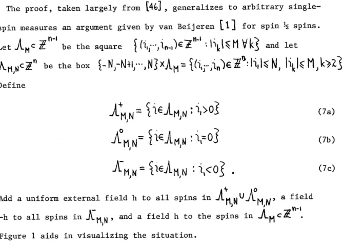
of (it,H,,V) is absolutely continuous with respect to Lebesgue measure in some interval

[-dd)

,d>0,

and that its Radon-Nikodym derivative has finite essential

supremum there. Then, as we see in Figure 1, by cutting off 'V completely

outside some sufficiently small interval [-TT7 c

_[-j

)J,

and properly

reshape

'T7

into Lebesgue measure

(Or [--TTJ

IT

restricted to

L-T)

T].

HatcAed

area=

CrosshatcWd

area

Figure 1

The largest possible T is given by

T=

sitJ)Idd

: A. C5 S

For tel? let bt be the two-point measure

A result of Griffiths

t

18

shows that if (A,$,

,d-[-T)T7

)

(20)

(21)

is a ferro-magnet with arbitrary polynomial Hamiltonian and Lebesgue single-spin measure, then

)Ac .(it). (22) Thus,

with our choice (20) of T,

Thus, with our choice (20) of T,

<o; I~bT/Z>•K:O-Ajy7>

A

6 ý.

A).(23)

We state this inequality as a proposition:

Proposition 2: Let (4,H,-V) be a finite Ising ferromagnet such that the single-spin measure -Y is absolutely continuous with respect to

Lebesgue measure on some interval

[-dd1

,

d>O,

and has essentially

bounded Radon-Nikodym derivative

there. Let T

=

s.Vt

[4d]:zt-e]•0r

I

4

1

B

and let bt be the two-point measure defined by (21). Then for all families A E()(A),

<a,-

;

H.

)f

3

>( <A 4>

(24)

Finally, we remark that Theorem 1 also holds in the case where the spins in the product 0 are replaced by more general functions of the type considered in Proposition 3.1. In addition, the proof of Theorem 1 goes through with minor modifications to give an analogous result for

Chapter III: Gaussian Inequalities Section 1: Introduction

In this short chapter, taken largely from [4E , we use combinatoric methods to prove an inequality bounding expectations of products of many spins by sums of products of simpler expectations. As a special case of a more general result, we show that the higher moments of the Gibbs measure

of a finite Ising ferromagnet (A.,H,b) with spin

½

spins (b=~-S(÷`l( ~- •]) ), a pair Hamiltonian, and zero external field are bounded in terms of the

covariance of L :

Here G is

the set of all partitions 9 of A

into pairs £k,k'

.

Inequality (1) is called a Gaussian inequality because the right-hand side

"-TI

< O

>

is the expectation of

T0 with

respect to a Gaussian

measure on A having mean zero and the same covariance

_o'CN

_,

₃

N~bH)

as the Gibbs measure of (J,H,b). It is closely related to Corollary 11.2.7, and may indeed follow from Theorem 11.2.6, though this is not presently

known. The Griffiths "analog system" method [ 18 (described in Section 11.2) shows that in addition to spin

½

models,(1) holds for ferromagnets (A ,H,v) whose single-spin measure V may be approximated by spin

½

models, including

h= T

4-TJTJ

([18

]i LeLesue

Meaoure

on

E-T)TD)

(2b)

vM·op-a~b)(aoS~~xpa4~b

s)J-/jp(=

s)s

)

cto

([431)

(2c)

38

Inequality (1) was discovered in its present form by Newman

[3O,

though a special case was established much earlier by Khintchine [ 4]. The proof given here is similar in spirit to that of Newman, but conceptually and technically simpler.

In Section 2 we prove the Gaussian (or Khintchine) inequality, comment on the roles played by various hypotheses in it, and mention possible improvements.

Section 2: Proof of Gaussian Inequality

We derive the Gaussian inequality from a more general result. Let us first define admissibility. Fix a finite family A of even cardinality, and use _{to denote complementation in A. A collectionv of even subfamilies} of A is called admissible if and only if every partition ofA into pairs is a refinement of some two-element partition B,B with BEt . For example, an admissible partition of A = 1,2,3,41 is = t,2,

1

41,33,

Theorem l:Let A be an even family of sites in a finite ferromagnetic Ising model (AJ,H,17) with pair Hamiltonian

and single-spin measure-V of the form ii

i •(P+d+"

(la)

Lr(0

=

-T

T

_(1b)

Y•

vo)exp(-aU1

bO-)/Sex

_-¾bsg)s

_•

_>

_(ic)

If a collection- _{of subfamilies of A is admissible, then}

Ko

r>

Z

<~>(2)

•

Proof:

By the "analog system" method

[

18 ]it suffices to prove Theorem 1 for the simplest measure of the form (1), namely

Furthermore, the "ghost spin" method of Griffiths

I

[1], which creates the effect of an external field by coupling to an extra "ghost" spin, permits us to assume the magnetic field hi is zero. As a final simplification, we reduce to the case when the family A is a set (all members distinct). If kl=k₂ are members of A, let

in abusive notation. We may assume without loss of generality that kl ,k2' always lies in B, not B. With this assumption, define

Then ) is admissible with respect to I=A-Jkl,k2 . Since >=(r and

A

A

this reduction procedure allows us to suppose that all members of A are distinct. With these simplifications in hand, we turn to the body of the proof.

We claim that all derivatives with respect to coupling constants J..

of Z

2 (

<~0r -

'~O

)

>)

_{are nonpositive when evaluated at zero coupling,}

and hence throughout the ferromagnetic region J. i 0. It is convenient to represent a differential operator in the coupling constants by a graph P . The vertices of

1

are sites in the model, and for each derivative --. appearing in D we place an edge between vertices

(sites) i and j. Sites with no incident edges are then suppressed. For example, the differential operator a would be represented

by the graph

1

Figure 1.

To simplify the notation, given a family of sites K we write (K] for

Ke•J

I

)

and

1'P[K]

for the action of the derivative associated with

the graph

T

on

JOe-d•bH(&).

Finally,

define the (z reduced) boundary

a of a graph I to be the set of all vertices of

'

having an odd number

of incident edges.

With this notation our claim becomes

T'

3

0

(6)

for all derivative graphs P , and is a consequence of the following three statements.

(1)

T*•(•RA)L

_and

_T*

([]BI[N)

_I

_both

_{vanish unless}

aT=A

(2)

If a*=A

then there exists a subgraph

G

of

and a set

_{Ba~with G=B .}

(3)

G'(1

]lA

-[

'])]=0

soT'(

}[A]-IBB

1)

Since the remaining terms on the left of inequality (6) are manifestly negative, this cancellation verifies the claim.

Statement (1) is obvious, since we are dealing with spin

½

spins.

Statement (2) is a straightforward induction. Since

~T'A

, given a site kE A there exists a site k't A connected with k by some path

g

in' .

Upon removing k and k' from A and I from _ , we see that by repeating the argument we may produce a partition of A into pacirs lk,k'v connected inm by edge-disjoint paths

I

. Since $ is admissible there exists BE• which is a union of some of these pairs; for G we just take the paths

connecting them.

Statement (3) is a simple calculation. Using A for symmetric difference we find

since

t--Iz

Corollary 2: Let A be of Theorem 1, and let

=

an

(

[A]i)=A-

(&G.

[])

(AG.

and

(-c)

G,

) A

t 0

(7)

QED

a family of sites with even cardinality in the model be the set of all partitions of A into pairs. Then

, E TT I<0

(8)

Proof:

This corollary is immediate from successive applications of Theorem 1.

Note that for a family of jointly Gaussian random variables with mean zero, Corollary 2 is an equality. In this sense, it is a best-possible result. However, Corollary 11.2.9, which states that

<ai 0'

K

<

r

(

>

4'-

<0 G-

+<Coi-

0ýoo<a

-

Z <ojýý

makes it clear that Corollary 2 may be improved for nonzero external field. Unfortunately, the proofs of Corollary 11.2.9 and Corollary 2 are dissimilar.

The former uses duplicate variables, while the latter is combinatoric in nature. A combinatoric proof of Corollary 11.2.9 might be valuable, and could lead to a new family of correlation inequalities.

Finally, we remark that some restriction on the Hamiltonian in Theorem 1 is necessary, because Corollary 2 fails for the four-site model (*,H,b), where

(9)

This is because the corollary demands that

but computing explicitly we find

<C;u1Xo o-7*

0

<o4o->

+0$Y3o

$o(c41o

(11)

and

in contradiction to (10).

Chapter IV: Ursell Functions Section 1: Introduction

In this chapter, taken largely from

[411,

we use the method of duplicate variables already exploited in Chapter II to study the Ursell functions

of finite ferromagnetic Ising models with spin 1 spins and pair interactions. Let us recall the definition of Ursell functions. The Ursell function

un(O ,n..,0) of a family

ai3

of n random variables may be defined by

means of a generating function as

Ion

(..(eP[f

.oi1)

(1)

Here is the expectation integral; we assume the necessary expectations are finite. The Ursell function may be defined recursively by

IT

'11PI

FO.)

(2)

Here U.L(jI

I)

is

the set of partitions of

1,' ,,n?. A set P in a partition

Oe1

j"

*

) has elements pa'pb, etc., and IeP denotes the cardinality of P. Finally, u(• ,n ,n) may be defined explicitly by

Combinatorially, the Ursell functions are related to expectations in the

same way that cumulants are related to moments and connected Green's functions (truncated vacuum expectation values) are related to Green's functions

(vacuum expectation values). As examples, we have

Also, if the family qC~ CT 4 has even symmetry (that is, the expectation of the product of an odd number of '>5 is zero), we have

U

0l(

,)

-

a-)

(4d)

In Section 2 we describe and investigate representations involving duplicate variables for the Ursell function of a general family of random variables Jj( . Let 03 , cE O,1, .',n-1- , be a collection of n independent but identically distributed copies of the family •(ji , let W0 be a

primitive nt root of unity, and define

n-I0 o(oO

We shall find that

(6)

a result previously obtained in another way by Cartier

[4

. Thus we

represent an Ursell function as an expectation. In the event that the

family

Qi30

has even

symmetry and n is even we can cut the number of

copies in half.(Of course, if lori has even symmetry and n is odd, un(~j,... )op) vanishes.) Defining

tiL- OI , (7)

•--0

(5)

we find the simplified representation

U'67. ",

-

_{) j}

) =

i E

Rt.n

_tU)

(8)

(The variable t introduced here has no relation to the variable t introduced

in transformation (11.2.1)) We conclude the section by demonstrating a method to produce additional representations.

In Section 3 we use the general results of Section 2 to study the even Ursell functions of finite ferromagnetic Ising models with spin

½

spins, pair interactions, and zero external field. It has been conjectured that these Ursell functions obey the inequality

We have seen that this conjecture is correct for n=2 and n=4

(Theorem 11.2.1; Corollaries 11.2.9, 111.2.2). In a few very simple models

it is known for all n

[40,421,

essentially by explicit calculation. Using

the representation (8) we prove here that in addition to n=2,4 inequality (9) holds for n=6. (We actually establish the stronger result that all the

coefficients

(-i

•

Z

B

tn(ik)...jk)

of

the Maclaurin

expansion of Z un in the couplings Jij are nonnegative for n=2,4,and 6.) Other independent proofs that (9) is valid for n=6 recently have been

given by Percus

[313

and Cartier (unpublished). We use combinatoric methods to derive a reduction formula for Ursell functions with repeated arguments. This allows us to conclude that conjecture (9) holds for arbitrary n

provided the spin arguments of the Ursell function are selected from

at most seven distinct sites. We finish Section 3 by noting some additional inequalities which follow from the methods we have developed. Although our results are derived explicitly for models with spin

½

spins, by the "analog system" method of C183 they extend immediately to the more general single-spin measures (I1.1.2) of the preceding chapter.

Section 4 investigates in more detail the results of Section 3. We establish a graphical notation for the derivatives of lLtU _n with respect

to couplings, and give formulas for the evaluation of these graphs when n=4,6,and 8. The formulas make clear why our method of proof works for n=2,4,6 but is inadequate for higher n. We present partial results showing

that derivatives of Ut, which are sufficiently simple in a graphical sense have the anticipated sign. We conclude with the asymptotic result that if all couplings Jij are nonzero and the inverse temperature P is sufficiently small or sufficiently large, then the conjectured inequalities hold. This result, however, is not uniform in the order n or the system

size.

In Appendix B we describe algorithms for calculating the derivatives of n/ U_n . We tabulate the results of a computer study using these algorithms on derivatives not controlled by the methods of Sections 3 and 4; they all have the expected sign. The study, however, is indicative but not exhaustive. This is because the long running time for the evaluation of even a moderately complex derivative - on the order of an hour - made a thorough study impractical.

Section IV.2: Representations of Ursell Functions

We describe and analyze representations for the Ursell function of a family of random variables aiO , ) lt,nn . These representations employ independent but identically distributed copies of the original family. Let C ý0,1,..,c3 0(E , , be (c+l) such independent copies of the family ¶73@ , each copy having the same joint distributions as 01 . Given a set of coefficients S eC we may define a new family of random

C

variables Isi3 i

.

by si = s ic( . We shall see that up to

a simple factor the family JsiJ has the same Ursell function as the

original family JCT3 . By judicious choice of the transformation coefficients

Sia we may cause all but the leading term in the Ursell function of the family Jsi} to vanish, thereby transforming an Ursell function into an expectation. In the event that the family 0O} has an even symmetry the representation simplifies, the number of copies employed being halved.

To exhibit the proportionality between the Ursell functions of os and sSi we recall that if a family of random variables may be split into

two mutually independent subfamilies, its Ursell function vanishes. ( This is immediate from definition (1.1) because the expectation factors.) Thus,

since only those terms for which ,=2= o = '" survive.

Next we give a specific choice for the transformation coefficients

Si(

such that u (S, ,.'S n) = (S,S 2 .. Sn). Take n copies of the original

family , and for choose , being a primitive nthoot of unity. Thus we have

n-1

SjZ• Co"(

C

(2)

o(=0

We claim that E

(S,

.Sk)

= 0 unless

k o

mod(n).

In establishing this it is convenient to regard the superscripts o( as running through the elements of N. Notice that E

•o~

_Cl '

_..

_{k) is unaltered if we subtract}

(in Zn) the same constant P n from each o( . Thus,

(3)

n-1

unless 6_0

M6od(),

since 7ok= 0 unless

w1odln)

.with thisW0

o=0

choice of variables we have

n

•(SS

"Si.)

(4)

It may happen that the family 0~\3 has even symmetry; that is, the

expectation of any product of an odd number of CT s is zero. In this case a simpler representation involving only 1 copies of the family

_Z

0?

is possible. (We take n even since for n odd by symmetry

un(O

>'')o)=0.)

,

Let

=

T_

,

(5)

where again CO is a primitive nth root of unity. To apply the preceding

argument to show (ti t"'tk) vanishes unless k 2 0 od(h' we note that

the superscripts q essentially may be regarded as elements of

jI/

because the ambiguity in the definition of W(0 '_"'+ k _{is obviated by the even}

symmetry of the family l* . Thus with even symmetry we find

Finally, we remark that if one chooses Si,= W , 6iE4 TF , only those

terms

i

~

(T)~

~~

in

the definition (1.3) of un(S1,..

,Sn)

survive which

satisfy the condition

•i

O

0 Mod(nP

V

Pe~.

By varying the f., different

representations for un(On _, ,' ) may be obtained. For example, the rep-resentations above have f. = 1 V i, and only the leading term survives.

On the other hand, with even symmetry by choosing

1-

I==0 and ;3

=

4

=

2

two terms survive,and we recover the transformation (11.2.1) and the representation (11.2.35) of Chapter II.

Section IV.3: Signs of Ursell Functions for Ising Ferromagnets We employ the representation (2.6) to analyze the Ursell functions u_n of a finite ferromagnetic Ising model (A,H,b) having spin

½

spins

and pair Hamiltonian

with zero external field. Construct for each even n the enlarged model (V•. A, H ,b) consisting of

I

non-interacting copies of the original model (A,H,b): the set of sites V, JL is just the disjoint union of n/z

copies ofA , and if we denote the spin at site i in the C- copy by 0 n/

the Hamiltonian eN is

Extend the definition (2.5) of the variables t. by setting

1 n-1

Thus what we called t. ₁ in (2.5) is ti ₁ here. Note that (n)*

_t

c

-For o(E6)3,5),5 b and 3E6O(I) "-(1 the matrix

l'W

1 is unitary. Thus,

1 in th

t

_i

5 ₍₂₎

and in the t-variables the representation (2.6) becomes

Lt J

Tr

i (3)

where we follow customary usage and write Tr(*) for (.)db. The

derivative of (3) with respect to coupling constants ,J, 1 is

In order to show that all these derivatives have a certain sign when evaluated

at arbitrary J, ,> 0 it suffices to show they all have this sign when the couplings J.. are set to zero, and this is what we do for n=2,4, and 6.

Theorem 1: Let u be the Ursell function of a finite Ising ferromagnet

(J.

,H,b) with

Let Z denote the partition function

e-Odb

of

(.A.,H,b).Then

for n=2,4, and 6

Moreover, if (J ,H,b) is connected, the inequality (5) is strict.

Remark: These inequalities, which as they stand involve factors of Z, may be converted to inequalities involving the spins alone by dividing by Z /

Proof:

a similar way, and the case n=2 is trivial.

We want to show that the sum

2:Z

i'4 tiim •

)

arising from the evaluation of (4) at J=0 is nonnegative. It is actually true that an individual term is nonnegative: Tr( * t ))O. Since this

trace factors over sites, we break it up into a product of traces of the form Tr( I' I . * ), with the common site subscript suppressed. By an argument given in Section 2 in connection with the representations

(2.2) and (2.6), this trace vanishes unless

I,+ "4•4%=0

YON40

.

Assume

this condition is satisfied at all sites. We claim that the function +V1"f' obeys the inequality

(1'

f*i

4

.go.

>(6)

To see this is true, we note that since (tl)* = t5 and (t3)* = t3, pairing

tl s with t5 s and t3s with one another reduces the problem to showing

that (tl)6 > 0 and (t1)3 t3< 0. This may be done by explicit verification

of cases. It now follows immediately that the product over the sites of the terms 1,,'1b is nonnegative and so has nonnegative trace, because the total number of

VIS

appearing with value 3 is even.

The strict positivity may be seen in several ways. One simple one is

to resurrect P=

/kTV

,

which we have set to one to this point.

Note that if a finite ferromagnetic Ising model with spin

½

spins is connected (see Chapter I for definition), then for any function of the spins F( , )

,<

F>

[F(-I,-

R

+. F0.