New Algorithm for Constructing and Computing Scale Invariants of 3D Tchebichef Moments

(1)

HAL Id: inserm-00839754

https://www.hal.inserm.fr/inserm-00839754

Submitted on 1 Jul 2013

HAL is a multi-disciplinary open access

archive for the deposit and dissemination of

sci-entific research documents, whether they are

pub-lished or not. The documents may come from

teaching and research institutions in France or

abroad, or from public or private research centers.

L’archive ouverte pluridisciplinaire HAL, est

destinée au dépôt et à la diffusion de documents

scientifiques de niveau recherche, publiés ou non,

émanant des établissements d’enseignement et de

recherche français ou étrangers, des laboratoires

publics ou privés.

New Algorithm for Constructing and Computing Scale

Invariants of 3D Tchebichef Moments

Haiyong Wu, Jean-Louis Coatrieux, Huazhong Shu

To cite this version:

Haiyong Wu, Jean-Louis Coatrieux, Huazhong Shu. New Algorithm for Constructing and

Comput-ing Scale Invariants of 3D Tchebichef Moments. Mathematical Problems in EngineerComput-ing, Hindawi

Publishing Corporation, 2013, pp.813606. �10.1155/2013/813606�. �inserm-00839754�

(2)

Volume 2013, Article ID 813606,8pages http://dx.doi.org/10.1155/2013/813606

Research Article

New Algorithm for Constructing and Computing Scale

Invariants of 3D Tchebichef Moments

Haiyong Wu,

1

Jean Louis Coatrieux,

1,2,3,4

and Huazhong Shu

1,4

1_{Laboratory of Image Science and Technology, School of Computer Science and Engineering, Southeast University,} Nanjing 210096, China

2_{INSERM, U1099, 35000 Rennes, France}

3_{Laboratoire Traitement du Signal et de l’Image, Université de Rennes I, 35000 Rennes, France} 4_{Centre de Recherche en Information Biomédicale Sino-Français (CRIBs), Nanjing 210096, China}

Correspondence should be addressed to Haiyong Wu; why@njxzc.edu.cn Received 13 December 2012; Accepted 27 March 2013

Academic Editor: Yi-Kuei Lin

Copyright © 2013 Haiyong Wu et al. his is an open access article distributed under the Creative Commons Attribution License, which permits unrestricted use, distribution, and reproduction in any medium, provided the original work is properly cited. Scale invariants of Tchebichef moments are usually achieved by a linear combination of corresponding invariants of geometric moments or via an iterative algorithm to eliminate the scale factor. According to the properties of Tchebichef polynomials, we propose a new approach to construct scale invariants of Tchebichef moments. An algorithm based on matrix multiplication is also provided to eiciently compute the 3D moments and invariants. Several experiments are carried out to validate the efectiveness of our descriptors and algorithm.

1. Introduction

Since the introduction of geometric moment invariants by Hu [1], moments and moment’s functions have been extensively applied in pattern recognition [2,3]. Due to the nonorthogonal kernel function of geometric moments, they sufer from high degree of information redundancy and are sensitive to noise, especially when higher order moments are concerned. Teague [4] introduced orthogonal continuous Legendre and Zernike moments, which can represent the image with minimal information redundancy and can be easily used for image reconstruction. he main drawback of the aforementioned moments is the discretization error, which accumulates with the increasing of moment order [5]. To resolve this problem, discrete orthogonal polynomials have been utilized to construct moments, such as Tchebichef [6], Krawtchouk [7], and Hahn [8]. heir basis functions exactly satisfy the orthogonality, which means they do not require any numerical approximation and spatial domain transformation. It makes them superior to the conven-tional continuous moments in terms of image representation capability.

Recently, the problem of moment invariance has been extensively investigated. For example, the invariants of Leg-endre moments have been achieved through image nor-malization method and indirect method. Chong et al. [9] proposed a direct method to construct the translation and scale Legendre moment invariants. Ong et al. [10] generalized this method to 3D directly. Following this way, Zhu et al. [11] derived translation and scale invariants of Tchebichef moments. However, Khalid pointed out that one weakness of this method is the high computational cost, especially when image size is large and higher order moments are concerned. herefore, this method is suitable only for a set of binary images with small size [12]. Another diiculty of aforementioned scale invariants is how to determinate their parameters, which need to be selected carefully to keep a compromise between numerical stability and complexity.

Inspired by the method proposed by Zhang et al. [13], we propose in this paper an improved approach to construct 3D scale invariants of Tchebichef moments. Instead of normal-izing by lower order moments, scale factors are eliminated by utilizing the orthogonality of coeicients. his method avoids enormous computing caused by iteration. Moreover,

(3)

2 Mathematical Problems in Engineering

we propose an algorithm based on matrix multiplication to eiciently compute the 3D moments and invariants.

he remaining of this paper is organized as follows: in

Section 2, Tchebichef polynomials and derivation of corre-sponding scale invariants are described in detail.Section 3

discusses an eicient way for computing 3D moments and invariants. Experimental results for evaluating the perfor-mance of the proposed descriptors are given inSection 4. Finally, conclusions are provided inSection 5.

2. Improved Scale Invariants of

3D Tchebichef Moments

In this section, the falling factorial is introduced to build a mutual relationship between Tchebichef polynomials and power series. In order to separate the scale factor, Tchebichef polynomials need to be transformed into power series irstly. hen, these separated power series are expressed through Tchebichef polynomials. By this way, moments of scaled image can be expressed as a linear combination of the original moments. We use the Stirling numbers instead of tedious iterations to obtain scale invariants, because the recursive procedure is an inherent deiciency of descriptors reported in [9–11].

2.1. Some Properties of Tchebichef Polynomials. he squared-norm of scaled Tchebichef polynomials is deined as [6]

��(�) = (1 − �)_{√� (�, �)}� � ∑ � = 0 (−�)�(−�)�(1 + �)� (�!)2_{(1 − �)} � , �, � = 0, 1, 2, . . . , � − 1, (1)

where(�)_�is the Pochhammer symbol given by (�)�= � (� + 1) (� + 2) ⋅ ⋅ ⋅ (� + � − 1) ,

� ≥ 1, (�)0= 1,

(2)

and�(�, �) is the squared-norm deined by

� (�, �) = _{(2� + 1) (� − � − 1)!.}(� + �)! (3) he falling factorial⟨�⟩_�is deined as [14]

⟨�⟩�= (−1)�(−�)�= � (� − 1) (� − 2) ⋅ ⋅ ⋅ (� − � + 1) ,

� ≥ 1, ⟨�⟩0= 1.

(4)

Using (4), (1) can be rewritten as ��(�) = � ∑ �=0��⟨�⟩�, (5) where ��= _{√� (�, �)}1 _(�!)(� + �)!(1 − �)2_{(� − �)!(1 − �)}� �. (6) Let�_�(�) = (�₀(�), �₁(�), . . . , �_�(�))�and�_�(�) = (1, ⟨�⟩₁, . . . , ⟨�⟩�)�be two column vectors, where the superscript T

indicates the transposition. Using (5), we have

��(�) = ��(�) , (7)

where�_�=(�_��), 0 ≤ � ≤ � ≤ �, is a lower triangular matrix whose size is(� + 1) × (� + 1). he matrix �_�is invertible because its diagonal elements are not zero; therefore,

��(�) = �−1��(�) = ��(�) , (8)

where�_�= (�_��), 0 ≤ � ≤ � ≤ �. �_�is a lower triangular matrix too, and its elements are given by [15]

��= (−1)�+�√� (�, �) (2� + 1) (�!)

2_{(1 − �)} �

(� + � + 1)! (� − �)!(1 − �)� . (9)

he falling factorial⟨�⟩_�and the power series��can be expanded mutually: ⟨�⟩� = � ∑ �=0�1(�, �) � �_, _�� ₌_∑� �=0�2(�, �) ⟨�⟩�, (10)

where�₁(�, �) is the Stirling number of the irst kind, satisfying the following recurrence relations:

�1(0, 0) = 1, �1(0, �) = �1(�, 0) = 0, � ≥ 1, � ≥ 1,

�1(�, �) = �1(� − 1, � − 1) − (� − 1) �1(� − 1, �) ,

(11) and�₂(�, �) is the Stirling number of the second kind, satis-fying

�2(0, 0) = 1, �2(0, �) = �2(�, 0) = 0, � ≥ 1, � ≥ 1,

�2(�, �) = �2(� − 1, � − 1) + ��2(� − 1, �) .

(12) he relationship between Tchebichef polynomials and power series has been established via the falling factorial, which is the fundamental of our descriptors.

2.2. Scale Invariants of 1D Tchebichef Moments. he 1D Tche-bichef moment of order � for an �-length signal �(�) is deined as �� = �−1 ∑ � = 0��(�) � (�) . (13)

Let�(�) be a scaled version of �(�) with a scale factor 1/�; that is,�(�) = �(�/�); then the Tchebichef moment of order � of �(�) has the form of

�� = �−1 ∑ � = 0��(�) � (�) = � �−1 ∑ � = 0��(��) � (�) . (14)

From (5), (8), and (10), we can see that ��(��) = � ∑ � = 0 � ∑ � = 0 � ∑ � = 0 � ∑ � = 0��1(�, �) � �_� 2(�, �)��(�) . (15)

(4)

Substituting (15) into (14), we have �� = � ∑ � = 0 � ∑ � = 0 � ∑ � = 0 � ∑ � = 0��1(�, �) � �+1_� 2(�, �)��. (16)

Equation (16) shows that the Tchebichef moment of the scaled signal can be expressed as a linear combination of the original ones. Based on this relationship, we derive the following theorem.

heorem 1. _{For a given integer}�, let �� = � ∑ � = 0 � ∑ � = 0 � ∑ � = 0 � ∑ � = 0��1(�, �) Γ −(�+1) � �2(�, �)��, (17)

withΓ_�= �₀�. hen�_��is invariant to image scaling. he proof is given in the appendix.

2.3. Scale Invariants of 3D Tchebichef Moments. he(� + � + �)th Tchebichef moment of a 3D image �(�, �, �) is deined by �� = �−1 ∑ � = 0 �−1 ∑ � = 0 �−1 ∑ � = 0��(�) ��(�)��(�) � (�, �, �) . (18)

Let us assume that the original image� is scaled with fac-tors1/�, 1/�, and 1/�, along direction, direction, and �-direction, respectively. hat is,�(�, �, �) = �(�/�, �/�, �/�). he(� + � + �)th moments of scaled image � are given by

�� = �� −1 ∑ � = 0 �−1 ∑ � = 0 �−1 ∑ � = 0��(��) ��(��)��(��) � (�, �, �) . (19) Similarly to 1D case, we can rewrite (19) as

�� = � ∑ � = 0 � ∑ � = 0 � ∑ � = 0 � ∑ � = 0��1(�, �) � �+1_� 2(�, �)�� ×∑� � = 0 � ∑ � = 0 � ∑ � = 0 � ∑ V= 0 ��1(�, �) ��+1�2(�, �) ��V ×∑� � = 0 � ∑ ℎ = 0 ℎ ∑ � = 0 � ∑ � = 0��1(�, ℎ) � ℎ+1_� 2(ℎ, �) ��V�� . (20) To construct the 3D moment invariants, we need the follow-ing lemma. Lemma 2. _Let Γ�= � � 100 �000� − �10�00, Θ�=� � 010 �000� − �10�00, Λ�= � � 001 �₀₀₀� − �10�00. (21)

hen, one hasΓ_�= �Γ_�,Θ_�= �Θ_�, andΛ_�= �Λ_�.

Proof. Using (6), (9), and (19), we have Γ�= � � 100 �000� = �10�00�000� + ��11�10�000� + ��100� �000� = �10�00+ � (� � 100 �000� + �11�10) . (22)

Taking�₁₀�₀₀+ �₁₁�₁₀ = 0 into account, we have Γ_� = �Γ_�. he other two relationships can be demonstrated in a similar way.

Using (20) and Lemma 2, we can construct the scale invariants of 3D Tchebichef moments, which are described in following theorem.

heorem 3. _{For given integers}�, �, �, let �� = � ∑ � = 0 � ∑ � = 0 � ∑ � = 0 � ∑ � = 0��1(�, �) Γ −(�+1) � �2(�, �)�� × ∑� � = 0 � ∑ � = 0 � ∑ � = 0 � ∑ V= 0 ��1(�, �) Θ−(�+1)� �2(�, �) ��V ×∑� � = 0 � ∑ ℎ = 0 ℎ ∑ � = 0 � ∑ � = 0��1(�, ℎ) Λ −(ℎ+1) � �2(ℎ, �) ��V�� , (23) whereΓ_�,Θ_�, andΛ_�are deined inLemma 2. hen,�� is invariant to image scale.

he proof is similar to that ofheorem 1since the kernel function is separable, and so it is omitted here.

3. Computing 3D Moments and Invariants

To achieve the scale invariance of 3D moments, (23) implies that it needs to compute a 12-level nested loop. Since the structure of (23) is symmetric, we introduce a new algorithm based on matrix multiplication to reduce the number of loops.

3.1. Computing 3D Moments. Let us begin with discussion of the 1D case. Let M= (M₀, M₁, . . . , M_�)Tbe a column vector constituted by the(0 ∼ �)th moments of �(�). From (5), it is well known that

M=[[_[ [ �0 �1 ⋅ ⋅ ⋅ �� ]] ] ] =[[_[ [ �0(1) �0(2) ⋅ ⋅ ⋅ �0(� − 1) �1(1) �1(2) ⋅ ⋅ ⋅ �1(� − 1) ⋅ ⋅ ⋅ ��(1) ��(2) ⋅ ⋅ ⋅ ��(� − 1) ]] ] ] [[ [ [ � (0) � (1) ⋅ ⋅ ⋅ � (� − 1) ]] ] ] . (24)

(5)

Yap et al. [7] proposed a matrix form of moments for a 2D image

� = �1��2�, (25)

where� is an � × � matrix of Tchebichef moments, �₁ = {��(�)}� = �−1, � = �−1� = 0, � = 0 , �2 = {��(�)}� = �−1, � = �−1� = 0, � = 0 , and � =

{�(�, �)}�, � = �−1�, � = 0 .

Exchanging the order of summation, we rewrite (18) as �� = �−1 ∑ � = 0��(�) { �−1 ∑ � = 0 �−1 ∑ � = 0��(�) ��(�)� (�, �, �)} . (26)

By combining (24) with (25), an efective algorithm to calculate (26) can be derived as follows.

Step 1. Computing� 2D images along �-direction by (25), we can get temporary matrices (seeFigure 8), where��_��(�) denotes the element of�th row and �th column in the �th plane of�-direction.

Step 2. Along�-direction, we rearrange the temporary matri-ces obtained inStep 1and get a(� + 1) matrix with size of �×(�+1). hen the required 3D moments are achieved ater they are premultiplied by the kernel function matrices; that is, [[ [ [ �000 ⋅ ⋅ ⋅ �0�0 �001 ⋅ ⋅ ⋅ �0�1 ⋅ ⋅ ⋅ �00� ⋅ ⋅ ⋅ �0�� ]] ] ] =[[_[ [ �0(0) �0(1) ⋅ ⋅ ⋅ �0(� − 1) �1(0) �1(1) ⋅ ⋅ ⋅ �1(� − 1) ⋅ ⋅ ⋅ ��(0) ��(1) ⋅ ⋅ ⋅ ��(� − 1) ]] ] ] ×[[_[[ [ �� 00(0) ⋅ ⋅ ⋅ ��0�(0) �� 00(1) ⋅ ⋅ ⋅ ��0�(1) ⋅ ⋅ ⋅ �� 00(� − 1) ⋅ ⋅ ⋅ ��0�(� − 1) ]] ]] ] , [[ [ [ �100 ⋅ ⋅ ⋅ �1�0 �101 ⋅ ⋅ ⋅ �1�1 ⋅ ⋅ ⋅ �10� ⋅ ⋅ ⋅ �1�� ]] ] ] =[[_[ [ �0(0) �0(1) ⋅ ⋅ ⋅ �0(� − 1) �1(0) �1(1) ⋅ ⋅ ⋅ �1(� − 1) ⋅ ⋅ ⋅ ��(0) ��(1) ⋅ ⋅ ⋅ ��(� − 1) ]] ] ] ×[[_[[ [ �� 10(0) ⋅ ⋅ ⋅ ��1�(0) �� 10(1) ⋅ ⋅ ⋅ ��1�(1) ⋅ ⋅ ⋅ �� 10(� − 1) ⋅ ⋅ ⋅ ��1�(� − 1) ]] ]] ] , .. ., [[ [ [ ��00 ⋅ ⋅ ⋅ ��0 ��01 ⋅ ⋅ ⋅ ��1 ⋅ ⋅ ⋅ ��0� ⋅ ⋅ ⋅ �� ]] ] ] =[[_[ [ �0(0) �0(1) ⋅ ⋅ ⋅ �0(� − 1) �1(0) �1(1) ⋅ ⋅ ⋅ �1(� − 1) ⋅ ⋅ ⋅ ��(0) ��(1) ⋅ ⋅ ⋅ ��(� − 1) ]] ] ] ×[[_[[ [ �� 0(0) ⋅ ⋅ ⋅ �� (0) �� 0(1) ⋅ ⋅ ⋅ �� (1) ⋅ ⋅ ⋅ �� 0(� − 1) ⋅ ⋅ ⋅ �� (� − 1) ]] ]] ] . (27)

he matrix representation is usually considered very efective in sotware packages such as MATLAB. But in

Section 4, our experiment shows that it performs well in C++ too.

3.2. Computing 3D Invariants. Equation (23) has a similar structure to the deinition of 3D moments. Exchanging the order of summation, we can rewrite (23) as

�� = � ∑ � = 0 � ∑ V= 0 � ∑ � = 0�1(�, �) �2(�, V) �3(�, �) � � �V�, (28) where �1(�, �)= � ∑ � = � � ∑ � = � � ∑ � = ��1(�, �) Γ −(�+1) � �2(�, �)��, (29a) �2(�, V) = � ∑ � = V � ∑ � = V � ∑ � = V��1(�, �) Θ −(�+1) � �2(�, �) ��V, (29b) �3(�, �) = � ∑ � = � � ∑ ℎ = � ℎ ∑ � = ��1(�, ℎ) Λ −(ℎ+1) � �2(ℎ, �) ��. (29c)

herefore, the algorithm presented in the previous sub-section can be applied to compute the invariants. Let us denote matrices{�_��}�, � = �_{�, � = 0}, {�₁(�, �)}�, � = �_{�, � = 0}, diag(�_�1, �_�2, . . . , �_��+1), {�2(�, �)}�, � = ��, � = 0, and {��}�, � = ��, � = 0 by C, S1, Δ, S2, and D,

respectively. hey are all lower triangular matrices, and (29a) can be evaluated by a matrix way; that is,Ξ = � ∗ �₁∗ Δ ∗ �2∗ �, where Ξ denotes the matrix {�1(�, �)}�, � = ��, � = 0. he same

procedure will be repeated in computing (29b) and (29c).

4. Experimental Results

In this section, we irst evaluate the eiciency of our comput-ing algorithm, which is compared with geometric moment invariants [16], Legendre invariants [10], and Zhu’s invariants [11]. hen we illustrate the performance of the proposed descriptors based on a 3D MRI image. Classiication abilities of four invariants are tested on character sets inally.

A 3D silhouette image shown in Figure 1 is composed of 128 binary images with size of128 × 128. It is used to evaluate the computational speed of the algorithm described inSection 3.Figure 2shows the computational time required to calculate the invariants of order up to 18. It should be noted that the program is implemented in C++ on a PC with Intel Core 2 Duo P8400 2.4 GHz CPU, 4 GB RAM.

Figure 2implies that our descriptors require less computation time when the order of invariants increases, because we apply the proposed algorithm for computing the Tchebichef moments as well as the invariants. he geometric moments and corresponding invariants are calculated directly through nested loops. For Zhu’s invariants and Legendre invariants, we utilize our method to obtain their 3D moments irstly, and then nested loops are used to compute moment invariants.

(6)

Figure 1: A 3D silhouette. 2 4 6 8 10 12 14 16 18 0.4 0.6 0.8 1 1.2 1.4 1.6 he order of invariants M ea n time ela ps ed (s) Geometric invariants Legendre invariants Zhu’s invariants Proposed invariants

Figure 2: Comparison of mean time elapsed (s).

Since there are no nested loops in our algorithm, the required time increases little with the order growing.

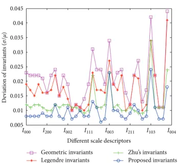
he Volume Library [16] contains regular volume data mainly coming from CT or MRI scanners.Figure 3 shows a 3D MRI head image selected from this library. We resize this head image with the factors of 0.5, 1, 1.5, and 2 along �-axis, �-axis, and �-axis, respectively, which form a test set consisting of 64 images with diferent sizes. In order to measure “invariant” performance of the descriptors, we also adopt the deviation�/�, which was proposed by Chong et al. [9]. Here � and � denote the standard deviation and mean of invariants with the same order, respectively.

Figure 4illustrates the standard deviation of the geometric invariants, Legendre invariants, Zhu’s invariants, and the proposed descriptors with the same order. It shows that the geometric invariants have the worst performance. Since high order of geometric moments has large variation in the dynamic range of values [6], this leads to unstable relative errors. Our descriptors have a slightly lower relative error than Zhu’s invariants and Legendre invariants.

Figure 3: A 3D MRI head image.

0.005 0.01 0.015 0.02 0.025 0.03 0.035 0.04 0.045

Diferent scale descriptors Geometric invariants Legendre invariants Zhu’s invariants Proposed invariants D evia tio n o f in va ri an ts ( �/ �) �000 �200 �002 �111 �003 �211 �103 �004

Figure 4: Standard deviation of lower order invariants for a non-uniformly scaled 3D MRI image.

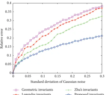
Moments of higher orders are generally considered more sensitive to image noise. To test the robustness of our invariants for degraded images, we add Gaussian noise (with mean� = 0 and variance � varying from 0.01 to 0.3) and salt-and-pepper noise (with diferent noise densities from 0.01 to 0.3) toFigure 1, respectively. We rearrange the scale invariants of an image following the scheme through the path (0, 0, 0) → (1, 0, 0) → (0, 1, 0) → (0, 0, 1) → (2, 0, 0) → (1, 1, 0) → (1, 0, 1) → (0, 2, 0) → (0, 1, 1) → (0, 0, 2) → ⋅ ⋅ ⋅ → (0, 0, �) and so on, to construct an invariant vector ��(�), where � is the maximum order of moment invariants.

In this experiment,� = 4 is chosen; that is, the length of ��(�) equals 35.

he relative error of the invariant vector corresponding to the original image� and the degraded image ̃� is deined as

� (�, ̃�) = ��_{��}− ��̃��

�� ,

(30)

(7)

6 Mathematical Problems in Engineering 0 0.05 0.1 0.15 0.2 0.25 0.3 0 0.05 0.1 0.15 0.2 0.25 0.3 0.35 0.4

Standard deviation of Gaussian noise

Re la ti ve err o r Geometric invariants Legendre invariants Zhu’s invariants Proposed invariants

Figure 5: Relative errors of four descriptors with respect to additive Gaussian noise. 0 0.05 0.1 0.15 0.2 0.25 0.3 0 0.05 0.1 0.15 0.2 0.25

Density of salt-and-pepper noise

Rela ti ve er ro r Geometric invariants Legendre invariants Zhu’s invariants Proposed invariants

Figure 6: Relative error of four descriptors with respect to additive salt-and-pepper noise.

Relative errors caused by Gaussian and salt-and-pepper noise are depicted in Figures5and6, respectively. We can observe that the relative error increases when increasing the noise level, and the proposed descriptors are more robust to noise than the other three competitors.

In the last experiment, we test the classiication ability of our descriptors in both noise-free and noisy conditions. A classiier is required to identify the class of an unknown input object. We utilize the second and third order of invariants to form a feature vector. herefore, the length of the vector equals 16. During the classiication, the feature of an unknown object is compared with the training feature

Figure 7: Original alphanumeric characters as a training set for invariant character recognition.

Table 1: Classiication results.

Noise-free 1% 2% 3% 4%

Geometric invariants 97.16 87.07 81.25 68.04 50.85 Legendre invariants 97.87 89.06 83.95 74.15 56.96 Zhu’s invariants 98.30 90.91 85.94 76.28 57.24 Proposed invariants 98.72 92.61 89.25 80.97 61.36

of a particular class. he Euclidean distance is frequently utilized as the classiication measure, which is deined by

� (��, ��(�)) = ��− ��, (31)

where�_�and�_�(�)are feature vectors of the unknown sample and the� class, respectively. We deine the classiication rule such that an unknown input object will belong to the nearest class. he average classiication accuracy is deined as

� = Number of correctly classiied images

he total number of images × 100%. (32) An original set of alphanumeric characters with size of 64 × 64 × 64 shown inFigure 7is used in this experiment. he reason for such a choice is that the elements in subsets {6, �, �}, {9, �, �}, and {�, �, �, 0, �} may be confused due to the similarity. Every element is scaled with the factors{0.5, 1, 1.5, and 2} along �-, �-, and �-axes, respectively, forming a testing set including 11 classes and 704 images. Additive salt-and-pepper noise with diferent noise densities 0.01, 0.02, 0.03, and 0.04 is added to the test set. he feature vectors based on the proposed invariants, geometric invariants, Legendre invariants, and Zhu’s invariants are used to classify these images. he comparison result is listed inTable 1. We can see that there are few diferences among the four descriptors in noise-free case. However, with the increase of noise density, our method is more robust than the other three.

5. Conclusions

We have presented a new method to derive the scale invari-ance of 3D Tchebichef moments. To reduce the computation time, we have proposed an eicient algorithm based on matrix multiplication for computing both 3D moments and 3D invariants. Experimental results show that our method has better classiication ability, it is more robust to noise than the existing moment-based methods, and it is very efective.

(8)

⌈ ⌊ ⌊ ⌊ �� 00(� − 1) �01� (� − 1) ... ��0�(� − 1) �10� (� − 1) �11� (� − 1) ... ��1�(� − 1) ... ... �� 0(� − 1) ��1� (� − 1) ... �� (� − 1) ⌉ ⌋ ⌋ ⌋ ⌈ ⌊ ⌊ ⌊ ⌊ �� 00(1) �01� (1) ... �0�� (1) �10� (1) �11� (1) ... �1�� (1) ... ��0(1) ��1(1) ... �� (1) ⌉ ⌋ ⌋ ⌋ ⌋ ⌈ ⌊ ⌊ ⌊ ⌊ ��00(0) �01� (0) ... ��0�(0) ��10(0) ��11(0) ... ��1�(0) ... �� 0(0) ��1� (0) ... �� (0) ⌉ ⌋ ⌋ ⌋ ⌋ � Figure 8

Appendix

Proof of

Theorem 1

TakingΓ_�= �Γ_�into account, we have �� = � ∑ � = 0 � ∑ � = 0 � ∑ � = 0 � ∑ � = 0��1(�, �) Γ −(�+1) � �2(�, �)�� = ∑� � = 0 � ∑ � = 0 � ∑ � = 0 � ∑ � = 0��1(�, �) � −(�+1)_Γ−(�+1) � �2(�, �)�� × ∑� � = 0 � ∑ � = 0 � ∑ � = 0 � ∑ � = 0��1(�, �) � �+1_� 2(�, �) ��. (A.1) Exchanging the order of summation, we can rewrite (A.1) as

�� = � ∑ � = 0 � ∑ � = 0��1(�, �) Γ −(�+1) � × ∑� � = 0 � ∑ � = 0 � ∑ � = 0 � ∑ � = 0 � ∑ � = 0�2(�, �)�1(�, �) � �−�_� 2(�, �) �� × ∑� � = ��. (A.2) Since � ∑ � = ��= ��, (A.3)

where�_��is the Kronecker symbol.

Substitution of (A.3) into (A.2) yields ��= � ∑ � = 0 � ∑ � = 0��1(�, �) Γ −(�+1) � × ∑� � = 0 � ∑ � = 0 � ∑ � = 0 � ∑ � = 0�2(�, �)�1(�, �)� �−�_� 2(�, �) ��. (A.4) Again, exchanging the order of� and �, we have

�� = � ∑ � = 0 � ∑ � = 0��1(�, �) Γ −(�+1) � × ∑� � = 0� �−�_∑� � = ��2(�, �)�1(�, �) � ∑ � = 0 � ∑ � = 0�2(�, �) �� . (A.5) Using∑�_{� = �}�₂(�, �) �₁(�, �) = �_��, we obtain ��= � ∑ � = 0 � ∑ � = 0��1(�, �) Γ −(�+1) � � ∑ � = 0 � ∑ � = 0�2(�, �) �� = ��. (A.6)

Conflict of Interest

he authors declare that they have no inancial and personal relationships with other people or organizations that can inappropriately inluence their work. here is no professional or other personal interest of any nature or kind in any product, service, and/or company that could be construed as inluencing the position presented in or the review of this paper.

Acknowledgments

his work was supported by the National Basic Research Program of China under Grant 2011CB707904; the National

(9)

Natural Science Foundation of China under Grants 61073138, 61271312, and 61201344; the Ministry of Education of China under Grant 20110092110023; the Key Laboratory of Com-puter Network and Information Integration (Southeast Uni-versity), Ministry of Education; the Centre de Recherche en Information M´edicale Sino-franc¸ais (CRIBs). hanks are also extended to the anonymous reviewers for their useful comments which help to improve the quality of the paper.

References

[1] M. K. Hu, “Visual pattern recognition by moment invariants,” IRE Transactions on Information heory, vol. 8, no. 2, pp. 179– 187, 1962.

[2] F. L. Alt, “Digital pattern recognition by moments,” Journal of the ACM, vol. 9, no. 2, pp. 240–258, 1962.

[3] S. A. Dudani, K. J. Breeding, and R. B. McGhee, “Aircrat identiication by moment invariants,” IEEE Transactions on Computers, vol. 26, no. 1, pp. 39–46, 1977.

[4] M. R. Teague, “Image analysis via the general theory of moments,” Journal of the Optical Society of America, vol. 70, no. 8, pp. 920–930, 1980.

[5] S. X. Liao and M. Pawlak, “On the accuracy of Zernike moments for image analysis,” IEEE Transactions on Pattern Analysis and Machine Intelligence, vol. 20, no. 12, pp. 1358–1364, 1998. [6] R. Mukundan, S. H. Ong, and P. A. Lee, “Image analysis by

Tchebichef moments,” IEEE Transactions on Image Processing, vol. 10, no. 9, pp. 1357–1364, 2001.

[7] P.-T. Yap, R. Paramesran, and S.-H. Ong, “Image analysis by Krawtchouk moments,” IEEE Transactions on Image Processing, vol. 12, no. 11, pp. 1367–1377, 2003.

[8] P. T. Yap, R. Paramesran, and S. H. Ong, “Image analysis using Hahn moments,” IEEE Transactions on Pattern Analysis and Machine Intelligence, vol. 29, no. 11, pp. 2057–2062, 2007. [9] C. W. Chong, P. Raveendran, and R. Mukundan, “Translation

and scale invariants of Legendre moments,” Pattern Recognition, vol. 37, no. 1, pp. 119–129, 2004.

[10] L. Y. Ong, C. W. Chong, and R. Besar, “Scale invariants of three-dimensional legendre moments,” in Proceedings of the 18th International Conference on Pattern Recognition (ICPR ’06), pp. 141–144, August 2006.

[11] H. Zhu, H. Shu, T. Xia, L. Luo, and J. Louis Coatrieux, “Trans-lation and scale invariants of Tchebichef moments,” Pattern Recognition, vol. 40, no. 9, pp. 2530–2542, 2007.

[12] K. M. Hosny, “Reined translation and scale Legendre moment invariants,” Pattern Recognition Letters, vol. 31, no. 7, pp. 533– 538, 2010.

[13] H. Zhang, H. Shu, G. Coatrieux et al., “Aine Legendre mo-ment invariants for image watermarking robust to geometric distortions,” IEEE Transactions on Image Processing, vol. 20, no. 8, pp. 2189–2199, 2011.

[14] L. Comtet, Advanced Combinatorics: he Art of Finite and Ininite Expansions, D. Reidel Publishing, Dordrecht, he Netherlands, 1974.

[15] H. Shu, H. Zhang, B. Chen, P. Haigron, and L. Luo, “Fast com-putation of Tchebichef moments for binary and grayscale images,” IEEE Transactions on Image Processing, vol. 19, no. 12, pp. 3171–3180, 2010.

(10)

Submit your manuscripts at

http://www.hindawi.com

Operations

Research

Advances in

Hindawi Publishing Corporation

http://www.hindawi.com Volume 2013

Mathematical Problems in Engineering

Abstract and

Applied Analysis

ISRN Applied Mathematics

http://www.hindawi.com Volume 2013 International Journal of

Combinatorics

Journal of Function Spaces and Applications International Journal of Mathematics and Mathematical Sciences

Hindawi Publishing Corporation http://www.hindawi.com Volume 2013

ISRN

Geometry

http://www.hindawi.com Volume 2013 Hindawi Publishing Corporation

Discrete Dynamics in Nature and Society

Advances in

Mathematical Physics

ISRN

Algebra

Probability

and

Statistics

Journal of

ISRN

Mathematical Analysis

Journal of

Applied Mathematics

Sciences

Stochastic Analysis

International Journal of

The Scientiic

World Journal

ISRN

Discrete Mathematics

Hindawi Publishing Corporation http://www.hindawi.com

Differential

Equations

International Journal of