Conversational scene analysis

Conversational Scene Analysis

by

Sumit Basu

S.B.,

Electrical Science and Engineering,

Massachusetts Institute of Technology (1995)

M.Eng., Electrical Engineering and Computer Science,

Massachusetts Institute of Technology (1997)

Submitted to the

Department of Electrical Engineering and Computer Science

in partial fulfillment of the requirements for the degree of

Doctor of Philosophy in Electrical Engineering and Computer Science

at the

MASSACHUSETTS INSTITUTE OF TECHNOLOGY

September 2002

@

Massachusetts Institute of Technology 2002. All rights reserved.

Author ...

...

Department of Electr'cal Engineering and Computer Science

August 30, 2002

Certified by...

...

Alex P. Pentland

Toshiba Professor of Media Arts and Sciences

_ T§plsis.upervisor

Accepted by...

...

...

Arthur C. Smith

Chairman, Department Committee on Graduate Students

BARKER

OF TECHNOLOGY

Conversational Scene Analysis

by

Sumit Basu

Submitted to the Department of Electrical Engineering and Computer Science on August 30, 2002, in partial fulfillment of the

requirements for the degree of

Doctor of Philosophy in Electrical Engineering and Computer Science

Abstract

In this thesis, we develop computational tools for analyzing conversations based on nonverbal auditory cues. We develop a notion of conversations as being made up of a variety of scenes: in each scene, either one speaker is holding the floor or both are speaking at equal levels. Our goal is to find conversations, find the scenes within them, determine what is happening inside the scenes, and then use the scene structure to characterize entire conversations.

We begin by developing a series of mid-level feature detectors, including a joint voicing and speech detection method that is extremely robust to noise and micro-phone distance. Leveraging the results of this powerful mechanism, we develop a probabilistic pitch tracking mechanism, methods for estimating speaking rate and energy, and means to segment the stream into multiple speakers, all in significant noise conditions. These features gives us the ability to sense the interactions and characterize the style of each speaker's behavior.

We then turn to the domain of conversations. We first show how we can very accurately detect conversations from independent or dependent auditory streams with measures derived from our mid-level features. We then move to developing methods to accurately classify and segment a conversation into scenes. We also show preliminary results on characterizing the varying nature of the speakers' behavior during these regions. Finally, we design features to describe entire conversations from the scene structure, and show how we can describe and browse through conversation types in this way.

Thesis Supervisor: Alex P. Pentland

Acknowledgments

There are so many people who have contributed to this endeavor in so many ways, it would be impossible to list them all. I apologize for any omissions, and I hope you know that you are in my heart and mind even if not on this page.

Of those I do mention, I would first and foremost like to thank Sandy for all of

his guidance, support, and inspiration over all of these years. Sandy, you've taught me the importance of imagination and creativity in the pursuit of science, and about the courage it takes to try something really different. That spirit is something I will always carry with me.

The rest of my committee comes next, for all of the effort and thought they have put in to help with this process. First, Jim Rehg, of the College of Computing at Georgia Tech, who has been discussing this topic with me for quite some time. You've been a great friend and mentor, Jim, and I appreciate everything you've done for me. Leslie Pack Kaelbling, of the MIT AI Lab - you put in more time and effort than I ever would have expected, giving me detailed and insightful comments at all levels of the work. And finally, Trevor Darrell, also of the Al Lab. As always, Trevor, you shot

straight from the hip and gave me some really solid feedback on the work - precisely

why I wanted you on board. To my entire committee: all of your help, insight, and feedback are so very much appreciated.

Someone who could never fit into just one category is Irfan Essa, a research scien-tist in the group when I came in and now a tenured professor at Georgia Tech. Irfan, you have been mentor, collaborator, and friend to me: you showed me how to read technical papers, how to write technical papers, and helped me get my first major publication. More recently, you've been an incredible help getting me ready for the

"real" world. Where would I be without you?

As Sandy has often said, "there's only one group of people you go to grad school with." I think I've been exceptionally lucky to have been here with the smartest and kindest set of people I could have hoped for. First among the Pentlanditos, of course, are Brian and Tanzeem, my officemates and best friends, who have been an unparalleled source of learning and joy. We've spent so many years together learning about pattern recognition and human behavior, both in a technical and a philosoph-ical sense, that I wonder how I will navigate the world without you. Vikram, a more recent addition, has been a wonderful friend and colleague as well. Jacob, though he spent only a year here, is the closest friend I've ever had, and I hope we can continue telecommunicating for many years to come. Judy, Karen, and Liz have been wonder-ful to have around, both as friends and as skilled office managers. Then there's Deb, Ali, Chris, Nathan, Drew, Bernt, Nuria, Yuri, Tony, Tom, Peter, Kris, Ben, Paul, Francois, and so many others. You know who you are, and thank you for being there.

and reassurances over the years have been a welcome source of solace. There are an endless number of deadlines in graduate school, and with your help I've (finally) managed to get through them all.

Then there are the many wonderful people who have kept the wheels of this great institute turning, the unsung heroes of MIT: Will, Chi, and all of the others at Nec-Sys; Kevin, Matt, Julie, Henry, and the rest of the Facilities crew; and Deb, Pat, Carol, and others in our custodial staff whose friendly hellos have brought smiles to so many dreary winter days.

Outside the academic walls, there are many more friends who have helped in one way or another: Mark, the best of my many roommates and a great friend in difficult times; Aaron and Mike, from back in the Infinite Monkey days, who introduced me to the concept of a social life; and more recently Kumalisa, who sometimes managed to pull me from my work-addicted shell to hit a Somerville party or two. Without

a doubt, I must include The Band: Stepha, Anindita, Aditi, and Tracie - listening

to our jam session tapes I realize that those Sunday afternoons were among the best times I've ever had in Cambridge.

My family - Baba, Ma, Didi Bhi, and more recently Zach - there is so much you have done for me. Without you, I could never have come this far, and I always thank you for everything you've done and continue to do. You may be far away, but I feel your support when I need it most.

Almost last but certainly not least, to Kailin, Stepha, and Jo: each in your own way, you have taught me something very important about love, and I will always remember you for that.

Finally, to everyone who has been with me in this long process, thank you for believing in me.

Contents

2.1.1 Features . . . . 30

2.1.2 Training . . . . 35

2.1.3 Performance . . . . 36

2.1.4 Applications . . . . 47

2.2 Probabilistic Pitch Tracking . . . . 49

2.2.1 The Model . . . . 50

2.2.2 Features . . . . 50

2.2.3 Performance . . . . 52

2.3 Speaking Rate Estimation . . . . 54

2.4 Energy Estimation . . . . 57

2.5 Moving On . . . . 58

3 Speaker Segmentation 59 3.1 Energy-Based Segmentation . . . . 60

3.1.2 Energy Segmentation in Real-World Scenarios with One and

Two Microphones . . . . 66

3.2 DOA-Based Segmentation . . . . 67

3.2.1 Computing the DOA . . . . 68

3.2.2 DOA Segmentation with Two Microphones . . . . 70

4 Finding Conversations 73 4.1 Finding Conversations from Separate Streams . . . . 74

4.2 Finding Conversations in Mixed Streams . . . . 80

4.3 Applications . . . . 85

5 Conversational Scenes 86 5.1 Identifying Scenes: Roles and Boundaries . . . . 88

5.2 Predicting Scene Changes . . . . 90

5.3 Scene-Based Features . . . . 92

6 Conversation Types 95 6.1 Features . .. .... ... . . . .. . ... . . . . 95

6.2 Describing Conversation Types . . . . 97

6.3 Browsing Conversations By Type . . . . 101

List of Figures

2-1 The human speech production system. . . . . 22

2-2 Spectrogram of a speech signal sampled at 16kHz with a close-talking

m icrophone. . . . . 23

2-3 Spectrogram of a speech signal sampled at 8kHz with a close-talking

m icrophone. . . . . 24

2-4 Graphical model for the linked HMM of Saul and Jordan. . . . . 26

2-5 The clique structure for the moralized graph for the linked HMM. . . 27

2-6 The clique structure and resulting junction tree for a four-timestep

linked H M M . . . . . 28

2-7 Autocorrelation results for a voiced and an unvoiced frame. . . . . 30

2-8 Spectrogram and normalized autocorrelogram for telephone speech

show-ing a low-power periodic noise signal. . . . . 31

2-9 Spectrogram and our new noisy autocorrelogram for telephone speech

showing a low-power periodic noise signal. . . . . 32

2-10 FFT magnitude for a voiced and an unvoiced frame . . . . 34

2-11 Performance of the linked HMM model on telephone speech. . . . . . 36

2-12 Comparison of an ordinary HMM versus our linked HMM model on a

chunk of noisy data. . . . . 38

2-13 Comparison of the voicing segmentation in various noise conditions

us-ing our method against our implementation of the Ahmadi and Spanias

algorithm . . . . 40

2-14 Speech and voice segmentation performance by our model with an SSNR of -14 dB. . . . . 42

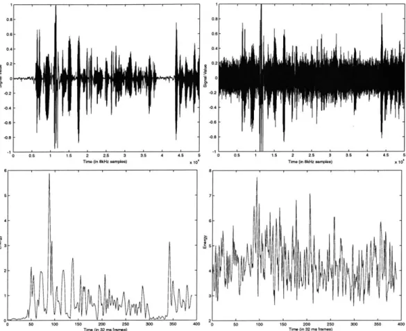
2-15 Speech signals and corresponding frame-based energy for an SSNR of

20dB and -14dB... ... 43

2-16 Performance of the speech segmentation in various noise conditions. . 44

2-17 Performance of the voicing and speech segmentation with distance from

the m icrophone. . . . . 45

2-18 The "sociometer," a portable audio/accelerometer/IR tag recorder,

de-veloped by Tanzeem Choudhury, with the housing designed by Brian C larkson. . . . . 46

2-19 The "smart headphones" application. . . . . 48 2-20 The normalized autocorrelation (left) and FFT (right) for a voiced frame. 51

2-21 Performance of the pitch tracking algorithm in the autocorrelogram. . 52

2-22 Weighted Gross Pitch Error (WGPE) for our model vs. Ahmadi and

Spanias vs. SSNR. . . . . 53

2-23 Gross Pitch Error (GPE) for our model vs. SSNR (dB) . . . . . 55

2-24 Estimated articulation rate, in voiced segments per second, for a

para-graph read at varying lengths. . . . . 56

2-25 Raw energy and regularized energy an SSNR of 20dB and -13dB. . . 58

3-1 Speaker segmentation performance with two microphones where the

signals are mixed at a 4:1 ratio and with varying amounts of noise. . 62

3-2 ROC curves for speaker segmentation performance with two

micro-phones for two noise conditions. . . . . 62

3-3 The raw per-frame energy ratio for part of our test sequence at an

SSNR of -14.7 dB. . . . . 63

3-4 The speaker segmentation produced by using raw energy for speaker 1

and speaker 2 at an SSNR of -14.7 dB . . . . 64

3-5 The speaker segmentation produced by using our regularized energy

3-6 ROC curves for speaker segmentation performance with our method and with raw energy using two sociometers where the speakers are

about five feet apart. . . . . 67

3-7 ROC curves for speaker segmentation performance with our method

and with raw energy using the energy from only one sociometer. . . . 68

3-8 The microphone geometry for the DOA-based segmentation experiments. 70

3-9 The peaks of the normalized cross-correlation over time. . . . . 71

3-10 Comparison of ROCs for DOA-based speaker segmentation using our

method without and with energy normalization. . . . . 72

4-1 Values of our alignment measure for various ranges of offset k over a

two-minute segment for a telephone conversation from the callhome

database. ... ... 75

4-2 Voicing segmentations for both speakers when perfectly aligned. . . . 76

4-3 ROC curves for detecting conversations in varying SSNR conditions,

tested over four hours of speech from eight different speakers. . . . . . 77

4-4 ROC curves for detecting conversations with different segment lengths. 78

4-5 ROC curves for conversation detection at different skip sizes. . . . . . 79

4-6 Values of our alignment measure for various ranges of offset k over

one-minute segments (3750 frames) for the sociometer data. . . . . . 80

4-7 Voicing segmentations from the sociometer data for both speakers when

perfectly aligned. . . . . 81

4-8 ROC curves for detecting conversations with different segment lengths. 83

4-9 ROC curves for conversation detection at different skip sizes. . . . . . 84

5-1 Voicing, speech, and pitch features for both speakers from an

eight-second segment of a callhome conversation. . . . . 87

5-2 Plots of the voicing fraction for each speaker in 500 frame (8 second)

blocks. . . . . 89

5-3 Results of scene segmentation for conversation EN 4807. . . . . 90

5-5 The ROC curves for the prediction of scene changes for 1000-frame

blocks. . . . . 91

5-6 The log likelihood of a scene change given the current features, plotted

along with the actual scene boundaries. . . . . 93

6-1 Results of scene segmentation and dominance histogram for two

con-versations, EN 4705 and EN 4721. . . . . 96

6-2 A scatterplot of all 29 conversations. . . . . 99

6-3 The result of clustering the conversations with a mixture of three

Gaus-sians. . . . . 100

6-4 Results of scene segmentation for conversation EN 4677, a low

domi-nance, short scene length conversation. . . . . 101

6-5 Results of scene segmentation for conversation EN 4569, a low-dominance,

long scene length conversation . . . . 102

6-6 Results of scene segmentation for conversation EN 4666, with high

List of Tables

2.1 Performance of voicing/speech segmentation on outdoor data. .... 47

2.2 Comparison of Gross Pitch Error (GPE) for various pitch tracking

algorithms on clean speech. . . . . 54

2.3 Speaking gap lengths for two sequences of the same text but spoken at

different speeds. . . . . 56

4.1 Probability table for vi (whether speaker one is in a voiced segment)

and v2 from the callhome data when the two signals are perfectly

aligned (k = 0). . . . . 76

4.2 Probability table for v, (whether speaker one is in a voiced segment)

and v2 from the callhome data when the two signals are not aligned

(k = 40000). . . . . 76

4.3 _{Probability table for vi (whether speaker one is in a voiced segment)}

and v2 from sociometer data when the two signals are aligned. . . . . 81

5.1 Scene Labeling Performance for the HMM. . . . . 89

5.2 Speaker two's variations across different conversational partners in two

scenes where she is holding the floor. . . . . 94

5.3 Speaker two's variations across different conversational partners in two

Chapter 1

Introduction

The process of human communication involves so much more than words. Even in the voice alone, we use a variety of factors to shape the meaning of what we say

- pitch, energy, speaking rate, and more. Other information is conveyed with our

gaze direction, the motion of our lips, and more. The traditional view has been to

consider these as "icing" on the linguistic cake - channels of additional information

that augment the core meaning contained in the words. Consider the possibility, though, that things may work in the other direction. Indeed, it may be these other channels which form the substrate for language, giving us an audio-visual context to help interpret the words that come along with it. For instance, we can watch people speaking to each other in a different language and understand much of what is going on without understanding any of the words. Presumably, then, by using these other signals alone we can gain some understanding of what is going on in a conversation.

This is the idea behind what we call "conversational scene analysis" as a parallel to

the well-established field of Auditory Scene Analysis (ASA) [5]. In the ASA problem,

the goal is to take an arbitrary audio signal and break it down into the various

auditory events that make up the scene - for instance, the honking of a car horn,

wind rustling by, a church bell. In Conversational Scene Analysis (CSA), we use a variety of input signals but restrict ourselves to the domain of conversations, in the hopes that we can make a much deeper analysis.

movie, a given conversation is made up of a number of scenes. In each scene, there are actors, each of whom is performing a variety of actions (typically utterances for

the purposes of our analysis). Furthermore, the roles that these actors play with

respect to each other vary from scene to scene: in a given scene, person A may be leading the conversation, while in another, A and B may be rapidly exchanging quips. In fact, it is these changes in role that will determine the scene boundaries.

The goal of this work is to develop computational means for conversational scene analysis, which breaks down into a number of tasks. First, we want to find where scenes exists, and whether a given pair of people are having a conversation. Next, we would like to find the scene boundaries, and even predict a change of scene. We would also like to characterize the roles the actors are playing, and find out who, if anyone, is holding the floor. We would like to find out the characteristics of the individual speakers in their scene, i.e., how they're saying what they're saying. Finally, we wish to characterize the overall conversation type based on its composition of scenes.

Why is this worth doing? There are a number of compelling reasons for this work

that imply a broad range of future applications. First, there is the spectre of the vast tracts of conversational audio-visual data already collected around the world, with more being added every day: meetings, classrooms, interviews, home movies, and more. There is an ever-growing need of effective ways to analyze, summarize, browse, and search through these massive stores of data. This requires something far more powerful than a fast-forward button: it is important to be able to examine and search this data at multiple scales, as our proposed ontology of actors, scenes, and conversation types would allow us to do.

Another motivation is the huge number of surveillance systems installed in stores, banks, playgrounds, etc. For the most part, the security people on the other end of these cameras are switching amongst a large number of video feeds. In most cases, the audio is not even a part of these systems for two reasons. First, it is assumed that the only way to use it would be to listen to the content, which could be a huge privacy risk, and second, because it would just be too much information - you can watch 10 monitors at once, but you can't listen to 10 audio streams and make sense of them.

With a mechanism to analyze conversational scenes, these security guards could get summary information about the conversations in each feed: on a playground, is an unknown individual trying to start conversations with several children? In an airport, are two or more individuals talking to each other repeatedly with their cellphones? In a store, is a customer giving a lecture to a salesperson? All of these situations can

be easily resolved with human intervention - if they can be caught in time.

Surveillance is not always a matter of being watched by someone else - sometimes

we want to have a record of our own interactions. The higher level analyses devel-oped here will result in a powerful feedback tool for individuals to reflect on their

conversations. There may be aspects of our style that we never notice - perhaps we

always dominate the conversation, never letting the other person get a word in edge-wise, or perhaps we are curt with certain people and chatty with others. While these differences in style may be obvious to third party observers, they are often difficult for us to notice, and sometimes socially unacceptable for others to tell us. Thinking further ahead, a real-time mechanism for analyzing the scene could give us immediate feedback about our ongoing conversations.

The personal monitoring vein extends to our fourth area, applications in health and wellness. Clinicians have long noted that depression, mania, fatigue, and stress are reflected in patients' speaking styles: their pitch, energy, and speaking rate all change under different psychological conditions. With the analysis techniques we will develop here, we can quantify these style parameters. This is quite different

from attempting to recognize emotions - we are merely characterizing how a person's

characteristics are changing with respect to his norm. Though this will not result in a litmus test for depression, it could be a very useful tool for the patient and the doctor to see how they vary from day to day and how certain behaviors/drugs are affecting their state of mind.

A final motivation for this work is in the development of socially aware

conver-sational agents and user interfaces. If we finally do achieve the vision of the robot butler, for instance, it would be nice if it could understand enough about our in-teractions to interrupt only at appropriate times. In a more current scenario, your

car could be constantly analyzing the conversational scenes you are involved in on your cellphone and in the car. Coupled with the wealth of current research in auto-matic traffic analysis, this could become an important tool for accident prevention. If you are holding the floor in a conversation or firing back and forth while entering a complicated intersection, the car could forcibly interrupt the conversation with a warning message, reconnecting you once the difficult driving scenario had passed. To

be even more concrete, any interface which needs to ask for your attention - your

in-stant messenger application, your cellphone, your PDA - could all benefit from being

conversationally aware.

This is still but a sampling of the possible reasons and applications for this work: furthermore, the more refined our techniques become, the more varied and interesting the application areas will be.

1.1

Our Approach

The area of conversational scene analysis is broad, and we will certainly not exhaust its possibilities in this work. However, we will make significant gains in each of the tasks we have described above. We now present the reader with a brief roadmap of how we will approach these tasks and the technologies involved. Note that for this study, we will be focusing exclusively on the auditory domain. Though we have spent significant efforts on obtaining conversation-oriented features from the visual domainin our past work, particularly in terms of head [3] and lip [4] tracking, we have yet to integrate this work into our analysis of conversations.

We will begin our work with the critical step of mid-level feature extraction. We first develop a robust, energy-independent method for extracting the voiced segments of speech and identifying groupings of these segments into speech regions using a multi-layer HMM architeture. These speech regions are the individual utterances or pieces thereof. The novelty of this method is that it exploits the changing dynamics of the voicing transitions between speech and non-speech regions. As we will show, this approach gives us excellent generalization with respect to noise, distance from

micro-phone, and indoor/outdoor environments. We then use the results of this mechanism to develop several other features. Speaking rate and normalized voicing energy are simple extensions. We then go on to develop a probabilistic pitch tracking method that uses the voicing decisions, resulting in a robust tracking method that can be completely trained from data.

At this point, we will already have developed the methods necessary for finding and describing the utterances of the individual actors in the conversation scene. We then begin our work on the conversational setting by briefly examining the problem of speaker separation, in which we attempt to segment the speech streams that are coming from different speakers. We look at this in two cases: in the first version, there are two microphones and two speakers; in the second, there is only one microphone. The features available to us are energy, energy ratios, and the direction of arrival estimate. The challenge here is to use the right dynamics in integrating these noisy features, and we show how our voicing segmentation provides a natural and effective solution.

The next task is to find and segment the conversational scenes. We start this with an investigation of how to determine that two people are involved in an interaction. We construct a simple measure of the dynamics of the interaction pattern, and find a powerful result that lets us very reliably determine the answer with only two-minute samples of speech. We then develop a set of block-based features for this higher level of analysis that characterize the occurences in the scene over a several second window. We use some of these features in an HMM that can identify and segment three kinds of states: speaker one holds the floor, speaker two holds the floor, or both are parlaying on equal footing. While the features themselves are noisy, the dynamics of the exchanges are strong and allow us to find the scenes and their boundaries reliably. We also show how we can predict these scene boundaries just

as they are beginning - though we see many false alarms as well, the latter give us

interesting information about possible changeover times. Once we have found the scene boundaries, we show how we can integrate features over the course of the scene to describe additional characteristics of it.

Finally, we develop two summary statistics for an entire conversation, i.e., a col-lection of scenes, and show how we can use the resulting histograms to describe conversation types. This highest level of description gives us an interesting bird's eye view of the interaction, and could prove to be a powerful feature for browsing very long-scale interactions.

This course of work will not cover all possible aspect of CSA, but it begins the path to an important new area. We will thus conclude with some ideas about specific directions that we hope to take this work in the years to come.

1.2

Data Sources

For the mid-level features through the conversation finding work, we will use data from a variety of sources: some of it from desktop microphones, some from condenser microphones, and some from body-mounted electret microphones - we will describe the details of these situations as they occur in our experiments. For the remainder of those experiments and for the entirety of the scene finding and characteriziation work, our primary source of data will be the LDC Callhome English database.

This database, collected by the LDC (Linguistic Data Consoritium) at the Univer-sity of Pennsylvania, consists of 63 conversations over international telephone lines. It is freely available to member institutions of the LDC and on a fee-basis to non-members. Native English speakers were recruited to call friends or family members overseas who were also native English speakers. The subjects agreed to completely release the contents of their conversation for research purposes: in return, they were able to have the international phone call free of charge and were compensated $10 for their time. The data is split into two channels, one for each speaker, each sampled at 8 kHZ with 8-bit mulaw encoding. There is a varying degree of noise due to the variance in quality of international telephone lines, sometimes appearing as constant static and sometimes as bursty segments of periodic noise, as we will describe later. Since the calls are all between friends and family members, the interactions are quite natural and represent a wide variety of interaction styles. These are precisely the

kinds of variations we are trying to analyze, and thus this is an ideal data source for our experiments.

1.3

Previous Work

As this project covers a wide array of technical areas, the list of related work is large. However, there has been little coordination of these areas into our manner of analysis, as we will see below. This section will give an overview of the work done in the related areas, while details of the respective techniques will be illuminated as necessary in the technical descriptions of later chapters.

In terms of the low-level auditory features, there has been a variety of work in doing related tasks. A majority of it has dealt only with the case of close-talking mi-crophones, as this has been the primary case of interest to the speech community. For our purposes, though, we require robustness both to noise and microphone distance. There has been prior work in finding voicing segments and tracking pitch in noisy con-ditions, and we will show how our new method significantly outperforms these results in terms of robustness and smoothness. Our application of the linked HMM to this problem is novel, and allows us to take advantage of the dynamics of speech produc-tion. It also gives us simultaneous decoding of the voicing and speech segmentation, with each helping the other's performance. Furthermore, as our features are indepen-dent from signal energy levels, our technique works in a wide variety of conditions without any retuning. We also present algorithms for probabilistic pitch tracking, speaking rate estimation, and speaking energy, all based on our segmentation and robust to significant environmental noise.

Speaker segmentation has also received some attention from the speech commu-nity, but in ways that are not ideal for our problem. The speaker identification methods (see [9] for a review) are effective only when there are 15-30 second

con-tiguous segments of speech to work over. The direction-of-arrival based methods

using multiple microphones are similarly effective when there are relatively station-ary sources, but have difficulty in distinguishing short segments from noise in the

cross-correlation and use artificial dynamic constraints to smooth over these changes. Since we are interested in capturing the sudden changes that occur in conversation, it is necessary for us to attempt something different. We show how we can leverage the results of our voicing-speech model to integrate over the noisy features of energy and phase (direction of arrival), resulting in performance that far exceeds that of the raw sigals.

As for the conversation detection and alignment results, we know of little other work in this area. While there has been some work on detecting conversations for a

PC user based on head pose and direction of arrival [23], we are working on a quite

different task: detecting whether two streams are part of the same conversation. To our knowledge, this is the first attempt to work on such a task, and our results are surprisingly strong. We show how we can pick out a conversational pair from amongst thousands of possibilities with very high accuracy and very low false alarm rates using only two minutes of speech. This has obvious applications in security, and we feel it is a major contribution to the speech processing community.

This brings us to our work on conversations and conversational scenes. While we are not the first to look at conversations, we are the first to look at their higher level structure in these terms. There has been a long history of work in linguistics and more recently in speech processing to determine discourse events using intonational cues (see the work of Heeman et al. [13] and of Hirschberg and Nakatani [14]). This work is at a much lower level of detail than we are considering here - their goal is to determine the role of particular utterances in the context of a dialogue; e.g., is new information being introduced? Is this answering a previous question? Our interest, on the other hand, is in finding the structure of the interaction: who is running the show, how are the individual actors behaving, and what overall type of interaction are they having?

The main other work in this final area is on multimedia and meeting analysis. The BBN "Rough'n'Ready" system, for instance, attempts to segment news streams into stories based on the transcription results of a speech recognition system [22]. While their results are very impressive, they are for quite a different task than ours.

Their goals involve tracking changes in the content of the dialogue, while we are more interested in the nature of the interaction. They are not able and not (yet) interested in analyzing conversational scenes. Hirschberg and Nakatani have also attacked this problem, seeking to use intonational cues to signal shifts in topic [15] with modest results. While this an interesting avenue, it differs from our notion of conversational scenes, which has more to do with the flow of interaction. We expect that the shifts in speaker dominance we seek will signify changes in topic, but we do not pursue this hypothesis in this work.

The other significant work on conversations comes from groups working on meet-ing analysis, among the most successful of which has been Alex Waibel's "Meetmeet-ing Browser" system [32]. While their overall goal is to help in browsing multimedia data of conversations, their path has been quite different from ours. Their primary focus has been on enhancing speech recognition in this difficult scenario and using the re-sults for automatic summarization. More recently, they have begun some preliminary work on speech act classification (e.g., was this a question, statement, etc?). They do not seem interested as of yet in the overall structure of the interaction, though to us it seems this could be a very powerful mechanism to aid in browsing conversations.

With this background, we are ready to embark on our study of conversational scene analysis. What follows covers a broad range of material, and we will make every attempt to refer to the appropriate literature when explaining our models and methods. We do expect a basic familiarity with signal processing and graphical models. If the reader feels they would like more background in these, we would heartily recommend the following: for graphical models, Jordan and Bishop's new book An Introduction to Graphical Models [17] is an excellent guide for novices and experts alike; for speech processing, Oppenheim and Schafer's classic text

Chapter 2

Auditory Features

There are many features in the auditory domain that are potentially useful for con-versational scene analysis, but we choose to focus on a few: when there is speech information, what energy and pitch it is spoken with, and how fast or slowly it is being spoken. Our choice comes from a long history of results championing these fea-tures in psycholinguistics, for instance the work of Scherer et al. in 1971 [30]. Scherer and his colleagues showed that pitch, amplitude, and rate of articulation were suffi-cient for listeners to be able to judge the emotional content of speech. While we are not focusing on emotions, we strongly believe that they are a parallel dimension to

the information we seek - i.e., if there is enough information to judge the emotional

content, there should be enough to judge the conversational interactions. Beyond this, the literature tells us little about which computational features to use, as our task of conversational scene analysis is still new.

By the end of this chapter, we will deal with each of these features in turn. We

must begin, though, at the beginning, by finding when there is even speech to be processed.

2.1

Speech and Voicing Detection

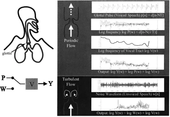
To understand the problem of speech and voicing detection, we must first examine the process of speech production. Figure 2-1 shows a simplified model of what occurs

glottis

Figure 2-1: The human speech production system. The lungs push air through the glottis to create either a periodic pulse, forcing it to flap open and closed, or just enough to hold it open in a turbulent flow. The resulting periodic or flat spectrum is then shaped by the vocal tract transfer function V(w).

during speech production, adapted from [25]. Speech can be broken up into two kinds of sounds: voiced and unvoiced. The voiced sounds are those that have a pitch, which we can think of loosely as the vowel sounds. The unvoiced sounds are everything else

- bursts from the lips like /p/, fricatives like /s/ or /sh/, and so on. During the voiced

segments, the lungs build up air pressure against the glottis, which at a certain point pops open to let out a pulse of air and then flaps shut again. This happens at a fixed period and results in an (almost) impulse train p[n, whose Fourier transform P[w] is thus also an (almost) impulse train with a period that is the pitch of the signal. This impulse train then travels through the vocal tract, which filters the sound with V[w] in the frequency domain, resulting in the combined output Y[w], which is the vocal tract filter's envelope multiplied by an impulse train, i.e.,

Y[w] = V[w] * P[w].

This is where the expressive power of our vocal instrument comes in: humans have a great deal of flexibility in how they can manipulate the vocal tract to produce a variety of different resonances, referred to as formants. The result is the full range of vowels and then some. In the unvoiced case, the lungs put out just enough pressure to push the glottis open and keep it open, as shown in the panel to the lower right. Once again, the sound is shaped by the configuration of the vocal tract, including

the position of the tongue and teeth. This results in sounds like

/s/

remaining cases of plosives, such as /p/ and /t/, result from pressure buildup and

release at other place in the vocal tract - the lips for /p/ and the tongue and palate

for /t/. The common element of all of these cases is that the resulting sound is not periodic. 250 7 200 4. t L150--oiced 100 silence 50

&

Time (in 32 ms frames)

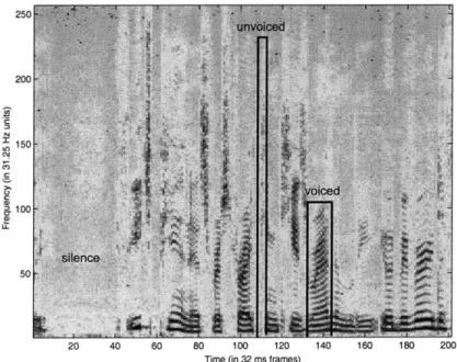
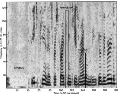
Figure 2-2: Spectrogram of a speech signal sampled at 16kHz with a close-talking mi-crophone. Note the banded nature of the voiced sounds and the clear high-frequency signature of unvoiced sounds.

Figure 2-2 shows the spectrogram of a speech signal sampled at 16 kHz (8 kHz Nyquist cutoff), with FFT's taken over 32ms windows with an overlap of 16ms be-tween windows. There are number of things to note in this image. First of all, in the voiced regions, we see a strong banded structure. This results from the product of the impulse train in frequency from the glottis P[w] multiplying the vocal tract transfer function V[w]. The bands correspond to the peaks of the impulse train. Since the pitch is in general continuous within a voiced region due to human limitations, these bands are continuous as well. Notice also how much longer the voiced regions are with respect to the unvoiced regions. In the unvoiced regions themselves, we see that the energy is strongly biased towards the high frequencies. It appears, however, that the energy of the unvoiced regions is almost as strong as that of the voiced regions. This somewhat misleading effect comes from two factors: first, this data was taken with a "close-talking microphone," the typical sort of headset microphone used for nearly all speech recognition work, and second, the signal has been "preemphasized," i.e., high-pass filtered, to increase the visibility of the unvoiced regions.

120 unv. Pe4 100 2 N80-Y 60 0 40-silence 20 20 40 60 80 100 120 140 160 180 200

Time (in 32 ms frames)

Figure 2-3: Spectrogram of a speech signal sampled at 8kHz with a close-talking microphone. Note that unvoiced sounds are now much less visible.

When we now look at the same piece of the signal sampled at 8kHz (figure 2-3), we now have half the frequency range to work with (4 kHz cutoff). As a result, it is much more difficult to distinguish the unvoiced components from silence. This problem only becomes worse when we move from close-talking microphones to

far-field mics - whereas the power of the periodic signals carries well over distance and

noise, the noise-like unvoiced signals are quickly lost. At even a few feet away from a microphone, many unvoiced speech sounds are nearly invisible.

Our goal is to robustly identify the voiced and unvoiced regions, as well as to group them into chunks of speech to separate them from silence regions. Furthermore, we want to do this in a way that is robust to low sampling rates, far-field microphones, and ambient noise. Clearly, to work in such broad conditions, we cannot depend on the visibility of the unvoiced regions. There has been a variety of work on trying to find the boundaries of speech, a task known in the speech community as "endpoint detection." Most of the earlier work on this topic has been very simplistic as the speech recognition community tends to depend on a close-talking, noise-free microphone situation. More recently, there has been some interest in robustness to noise, due to the advent of cellular phones and hands-free headsets. For instance, there is the work of Junqua et al. [18] which presents a number of adaptive energy-based techniques, the work of Huang and Yang [16], which uses a spectral entropy measure to pick out voiced regions, and later the work of Wu and Lin [34], which extends the work of Junqua et. al by looking at multiple bands and using a neural network to learn the appropriate thresholds. Recently, there is also the work of Ahmadi and Spanias [1], in which a combination of energy and cepstral peaks are used to identify voiced frames, the noisy results of which are smoothed with median filtering. The basic approach of these methods is to find features for the detection of voiced segments (i.e., vowels) and then to group them together into utterances. We found this compelling, but noted that many of the features suggested by the authors above could be easily fooled by environmental noises, especially those depending on energy.

We thus set out to develop a new method for voicing and speech detection which was different from the previous work in two ways. First, we wanted to make our

low-level features independent of energy, in order to be truly robust to different mi-crophone and noise conditions. Second, we wished to take advantage of the multi-scale

dynamics of the voiced and unvoiced segments. Looking again at the spectrograms,

there is a clear pattern that distinguishes the speech regions from silence. It is not in the low-level features, certainly - the unvoiced regions often look precisely like the silence regions. In speech regions, though, we see that voicing state is transitioning rapidly between voiced (state value 1) and unvoiced/silence (state value 0), whereas in the non-speech regions, the signal simply stays in the unvoiced state. The dynam-ics of the transitions, then, are different for the speech and non-speech regions. In probabilistic terms, we can represent this as follows:

P(V = 1iV 1-1 = 1, St = 1) # P(V = 1|Vt_1 = 1, St = 0) (2.2) This is clearly more than the simple HMM can model, for in it the current state can depend only on the previous state, not on an additional parent as well. We must turn instead to the more general world of dynamic Bayesian nets and use the "linked HMM" model proposed by Saul and Jordan [29]. The graphical model for the linked HMM is shown in figure 2-4. The lowest level states are the continous observations from our features, the next level up (V) are the voicing states, and the highest level (St) are the speech states.

eSt Is;

Figure 2-4: Graphical model for the linked HMM of Saul and Jordan.

This model gives us precisely the dependencies we needed from equation 2.2. Note that as in the simple HMM, excepting the initial timestep 0, all of the states in each layer have tied parameters, i.e.,

P(V =_ ijV _1 = J, St = k ) = P(Vt+1 i|Vt = J, St+1 = k ) ( 2.3)

P( St = i|st-1 = A = P( St+1 = ist = A 24

P(Ot = x|St = i) = P(Ot+1= xSt+1 = i) (2.5)

(2.6)

In a rough sense, the states of the lower level, V, can then model the voicing state like a simple HMM, while the value of the higher level St will change the transition matrices used by that HMM. This is in fact the same model used by the vision community for modeling multi-level dynamics, there referred to as switching linear dynamics systems (as in [26]). Our case is nominally different in that both hidden layers are discrete, but the philosophy is the same. If we can afford exact inference on this model, this can be very powerful indeed: if there are some places where the low-level observations P(OtlVt) give good evidence for voicing, the higher level state will be biased towards being in a speech state. Since the speech state will have much slower dynamics than the voicing state, this will in turn bias other nearby frames to be seen as voiced, as the probability of voicing under the speech state will be much higher than in the non-speech state. We will see this phenomenon later on in the results.

S ,' t S

Figure 2-5: The clique structure for the moralized graph for the linked HMM.

In our case, inference and thus learning are fairly easy, as both of our sets of hidden states are discrete and binary. The clique structure for the moralized, triangulated

graph of the model is shown in figure 2-5. The maximal clique size is three, with all binary states, so the maximum table size is 2' = 8. This is quite tractable, even though we will have an average of two of these cliques per timestep. The junction tree resulting from these cliques is shown for a four-timestep linked HMM in figure 2-6.

It is easy to see by inspection that this tree satisfies the junction tree property [17,

i.e., that any set of nodes contained in both cliques A and B are also contained in all cliques between A and B in the clique graph. Doing inference on this tree is analagous to the HMM except for an additional clique for each timestep (cliques 3,

5, etc.). To flesh out this analogy, we use node 9 as the root of the tree and collect

evidence from the observations and propagate them to the root (the forward pass); then propagate the results back to the individual nodes (backward pass). Scaling is achieved by simply normalizing the marginals to be proper probability distributions; the product of the normalizing constants is then the log likelihood of the data given

the model. This is an exact parallel to a -

#

12 i1 ., 18 1 4 - 1 7 -t 2 5 8 10 M 13- 6

7---~~)

Figure 2-6: The clique structure and resulting junction tree for a four-timestep linked HMM. To prevent clutter, the nodes are not shown and the cliques have been spaced

apart between timesteps. The root of the tree is node 9.

primary effort in inference will involve marginalizing two-by-two-by-two tables onto two-by-two tables, then using these to update two-by-two-by-two potentials. The

number of operations per timestep 0(t) is then

0(t)

=

[Ns,

where N,,1 is the number of states in the lower hidden layer and N,,2 is the number

of states in the upper hidden layer. The first term is for computing the likelihoods of each state from the features, while the second two are for updating the two 3-cliques belonging to each timestep. The factor of two is for doing the forward and backward passes of the junction tree algorithm. Since both our hidden layers have binary states, this results in 36 operations per timestep.

For a simple HMM, the order of operations would be

0(t) = 2 [Ns,1 + N . (2.8)

With a binary voiced/unvoiced state, this would require only 12 operations per timestep; with another binary HMM on top of this for the speech/non-speech de-cision the total would be 24 operations per timestep. We will show later, though, that such a model would not be as effective as the full linked HMM.

On the other hand, we could fully represent the linked HMM model with a

four-state HMM, representing each combination of voicing and speech four-states as a

sep-arate state. For instance, state 1 would be [speech=0,voice=0], state 2 would be [speech=0,voice=1], and so on. We could then tie the observation models for the voiced and unvoiced states (for states [speech=O,voice=0] and [speech=1,voice=1]), resulting in the same 2[2 + 42] or 36 operations per frame that we had for the linked HMM.

While 36 operations per frame versus 24 is a significant difference, it certainly does not make our model intractable: it is because of our small state size that we are saved from an explosion in the number of operations. We can thus apply the standard junction tree algorithm for inference without any need for approximations.

2.1.1

Features

We are using three features for the observations: the non-initial maximum of the normalized "noisy" autocorrelation, the number of autocorrelation peaks, and the

normalized spectral entropy. These are all computed on a per-frame basis - in our

case, we are always working with 8 kHz speech, with a framesize of 256 samples (32 milliseconds) and an overlap of 128 samples (16 milliseconds) between frames.

Noisy Autocorrelation

The standard short-time normalized autocorrelation of the signal s[n] of length N is defined as follows:

a[k] = nk (2.9)

(X:N-s[n 2),!(E=0n=k sn2)1

We define the set of autocorrelation peaks as the set of points greater than zero that are the maxima between the nearest zero-crossings, discounting the initial peak at zero (a[O] is guaranteed to be 1 by the definition). Given this definition, we see a small number of strong peaks for voiced frames because of their periodic component, as seen in figure 2-7. Unvoiced frames, on the other hand, are more random in nature, and thus result

maximum peak

in a large value and

number of small peaks (see figure). We thus use both the the number of peaks as our first two features.

Figure 2-7: Autocorrelation results for a voiced (left) and an unvoiced (right) frame. 1 0.8 S0.6 0 4--0.2 S40 60L so 4; 1 20 Offset (WampIes) 0.8 0.6 0.4 -0.2 -0.4 -0.8 _{40 60 8D 100 120} Ofmst (SamPles) 140 140

There is one significant problem to the standard normalized autocorrelation,

though - very small-valued and noisy periodic signals will still result in strong peaks.

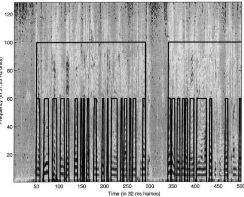
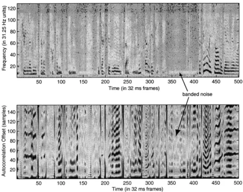
This is a necessary consequence of the normalization process. As much of the data we are analyzing comes from the LDC callhome database, which is composed entirely of international telephone calls, we see many forms of channel noise that have low energy but are still periodic. Furthermore, they have a fairly noisy structure for each period. An example is shown in figure 2-8 below. In the non-speech regions, we see a very light band of periodic energy at a low frequency, but in the autocorrelogram, we see rather strong correpsonding peaks, which could make the resulting features very attractive to the voiced model.

120 100 LO 4 80 60 40 2 20 LiL 50 100 150 200 250 300 350 \ 400 450

Time (in 32 ms frames)

banded noise

50 100 150 200 250 300 350 400 450 500 Time (in 32 ms frames)

Figure 2-8: Spectrogram (top) and normalized autocorrelogram (bottom) for tele-phone speech showing a low-power periodic noise signal. Note the light spectral band in the non-speech regions and the strong resulting autocorrelation peaks.

500 140 E 120 100 o 80 C 0 CCC 60 CO 8 0_S20

5120 N100 c 80--60 I E?20-50 100 150 200 250 300 350 400 450 500

Time (in 32 ms frames)

140 E a120 100 09 60A 40 /W 20 4 50 100 150 200 250 300 350 400 450 500

Time (in 32 ms frames)

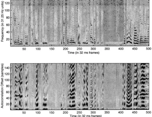
Figure 2-9: Spectrogram (above) and our new noisy autocorrelogram (below) for tele-phone speech showing a low-power periodic noise signal. Note how the autocorrelation peaks in the voiced regions are unaffected while the peaks in the non-speech regions have practically disappeared (compare to standard autocorrelogram in figure 2-8).

We could deal with this by simply cutting out frames that were below a certain energy, but this would make us very sensitive to the energy of the signal, and would result in a "hard" cutoff for a frame to be considered as voiced. This would lead us to a significant loss in robustness to varying noise conditions. We instead devised a much softer solution, which is to add a very low-power Gaussian noise signal to each frame before taking the autocorrelation. In the regions of the signal that have a strong periodic component, this has practically no effect on the autocorrelation. In lower power regions, though, it greatly disrupts the structure of a low-power, periodic noise source. In figure 2-9, we see the result of this procedure. The lower the signal power, the greater the effect will be on the autocorrelation, and thus we have a soft rejection of low power periodic components. To estimate the amount of noise to use, we use a two-pass approach - we first run the linked-HMM to get a rough segmentation of voicing and use the resulting non-speech regions to estimate the signal variance during silence. We then add a Gaussian noise signal of this variance to the entire signal and run the segmentation again.

Spectral Entropy

Another key feature distinguishing voiced frames from unvoiced is the nature of the FFT magnitudes. Voiced frames have a series of very strong peaks resulting from the pitch period's Fourier transform P[w] multiplying the spectral envelope V[w]. This results in the banded regions we have seen in the spectrograms and in a highly structured set of peaks as seen in the first panel of figure 2-10. In unvoiced frames, as seen in the right panel, we see a fairly noisy spectrum, be it silence (with low magnitudes) or a plosive sound (higher magnitudes). We thus expect the entropy of a distribution taking this form to be relatively high. This leads us the notion of spectral entropy, as introduced by Huang and Yang [16].

To compute the spectral entropy, we first normalize P[w] to make it into a proper distribution.

_P[w ]

p[w] - P[W (2.10)

9 8 - 76 -4

3i

2:-0.5

FIequency (in 31.25 Hz units) Frequency (in 31.25 Hz units)

Figure 2-10: FFT magnitude for a voiced (left) and an unvoiced (right) frame. The spectral entropy for the first frame is 3.41; the second has an entropy of 4.72.

Normalizing in this way makes this feature invariant to the signal energy, as by Parseval's relation we are normalizing out the energy of the signal. We can then compute the entropy of the resulting distribution:

Hs = - p[w] log p[w]. (2.11)

In figure 2-10, H, is 3.41 for the voiced frame and 4.72 for the unvoiced frame

-as we would expect, the entropy for the flat unvoiced distribution is much higher. Of course, there is some variation in the range of entropy values for various signals, so we maintain a windowed mean and variance for this quantity and then normalize the raw H, values by them.

We can take this one step further and compute the relative spectral entropy with respect to the mean spectrum. This can be very useful in situations where there is a constant voicing source, such as a loud fan or a wind blowing across a microphone aperture. The relative spectral entropy is simply the KL divergence between the current spectrum and the local mean spectrum, computed over the neighboring 500 frames:

where m[w] is the mean spectrum. The performance gain from using the relative entropy is minimal for our synthetic noise environments, as the additive noise has a flat spectrum. In outdoor conditions, though, it makes a significant difference, as we will show in our experiments.

2.1.2

Training

With our features selected, we are now ready to parametrize and train the model. We choose to model the observations with single Gaussians having diagonal covariances. It would be a simple extension to use mixtures of Gaussians here, but since the features appear well separated we expected this would not be necessary. Furthermore, reducing the number of parameters in the model greatly reduces the amount of training data necessary to train the model.

We first unroll the model to a fixed sequence length (as in figure 2-6) of 500 timesteps. This is not necessary in principle, as our scaling procedure allows us to deal with chains of arbitrary length, but this allows us to get a more reliable estimate for the parameters of the initial nodes P(vo) and P(so).

Because we can do exact inference on our model, the Expectation-Maximization or EM algorithm [8] is an obvious candidate for learning the parameters. The basic idea is to infer the distribution over the unlabeled hidden nodes (the expectation step) and then maximize the likelihood of the model by setting the parameters to the expectations of their values over this distribution. The tied parameters do not complicate this procedure significantly - it simply means that we accumulate the distributions over each set of nodes sharing the same set of parameters, again as with the HMM [27]. Furthermore, for our training data, the hidden nodes are fully labeled, as the voicing and speech state are labeled for every frame. As a result, the application of EM is trivial. However, we could easily train the model on additional, unlabeled data by using EM in its full form.

We trained the model using several minutes of speech data from two speakers in the callhome database (8000 frames of 8 kHz, 8-bit mulaw data) with speech and voicing states labeled in each frame. Since all states were labeled, it was only necessary to

run EM for one complete iteration.

2.1.3

Performance

To now use the model on a chunk of data, we first unroll it to an appropriate size. We then enter the evidence into the observed nodes, but instead of doing inference, or "sum-product," on the junction tree, we now use the "max-product" algorithm,

propagating the maximum of each marginal configuration instead of the sum [20].

This is a generalization of the Viterbi algorithm for HMMs, and finds the posterior mode of the distribution over hidden states given the observations. In other words, the sequence produced by the max-product algorithm is the one that has the highest likelihood of having produced the observations we entered.

1o19

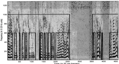
120-~80

Figure 2-11: Performance of the model on telephone speech. The upper line (at 100) shows the inferred speech state and the lower line (at 60) shows the voicing state.

A first example of our results on telephone speech is shown in figure 2-11. As we had hoped, the model has correctly segmented the many voiced regions, as well as identifying the speech and non-speech regions. While this is encouraging, we wish to see the detailed performance of the model under noise and distance from microphone. Before we do this, though, we would like to point out the major advantages of this model over a simple HMM for detecting voiced/unvoiced states. First of all, we are