HAL Id: hal-00710434
https://hal.archives-ouvertes.fr/hal-00710434
Submitted on 20 Jun 2012HAL is a multi-disciplinary open access archive for the deposit and dissemination of sci-entific research documents, whether they are pub-lished or not. The documents may come from teaching and research institutions in France or abroad, or from public or private research centers.
L’archive ouverte pluridisciplinaire HAL, est destinée au dépôt et à la diffusion de documents scientifiques de niveau recherche, publiés ou non, émanant des établissements d’enseignement et de recherche français ou étrangers, des laboratoires publics ou privés.
Ground referencing GRACE satellite estimates of
groundwater storage changes in the California Central
Valley, USA
B. R. Scanlon, L. Longuevergne, D. Long
To cite this version:
B. R. Scanlon, L. Longuevergne, D. Long. Ground referencing GRACE satellite estimates of ground-water storage changes in the California Central Valley, USA. Water Resources Research, American Geophysical Union, 2012, 48, pp.04520. �10.1029/2011WR011312�. �hal-00710434�
Ground Referencing GRACE Satellite Estimates of Groundwater Storage Changes in the 1
California Central Valley, US 2
3 4
Scanlon, B.R. 1, Longuevergne, L.2 and Long, D.2 5
6 7
1Bureau of Economic Geology, Jackson School of Geosciences, University of Texas at Austin,
8
Austin, Texas 78758, United States 9
2
Géosciences Rennes - UMR CNRS 6118, Université de Rennes 1, 35042 Rennes Cedex, 10
France 11
Abstract 13
There is increasing interest in using GRACE (Gravity Recovery and Climate Experiment) 14
satellite data to remotely monitor groundwater storage variations; however, comparisons with 15
ground-based well data are limited but necessary to validate satellite data processing, 16
especially when the study area is close to or below the GRACE footprint. The Central Valley is a 17
heavily irrigated region with large-scale groundwater depletion during droughts. Here we 18
compare updated estimates of groundwater storage changes in the California Central Valley 19
using GRACE satellites with storage changes from groundwater level data. A new processing 20
approach was applied that optimally uses available GRACE and water balance component data 21
to extract changes in groundwater storage. GRACE satellites show that groundwater depletion 22
totaled ~31.0±3.0 km3 for GRGS (Groupe de Recherche de Geodesie Spatiale) satellite data 23
during the drought from Oct 2006 through Mar 2010. Groundwater storage changes from 24
GRACE agreed with those from well data for the overlap period (Apr 2006 through Sep 2009) 25
(27 km3 for both). General correspondence between GRACE and groundwater level data 26
validates the methodology and increases confidence in use of GRACE satellites to monitor 27
groundwater storage changes. 28
Introduction 29
Water scarcity is a critical issue globally with an estimated 1.1 billion people lacking access 30
to safe drinking water globally (UN Development Program, 2006). Groundwater is increasingly 31
being used for drinking water and serves an estimated 1.5 – 2.8 billion people globally and up to 32
98% of rural populations (Morris et al., 2003). There has been a rising trend in groundwater use 33
for irrigation since the 1940s and 1950s and groundwater now accounts for ~40% of irrigation 34
water globally (Siebert and Döll, 2010). Increasing reliance on groundwater for drinking water 35
and irrigation is attributed to ubiquity of groundwater resources, ease of development with 36
minimal capital costs, generally good water quality because of filtering during recharge, and 37
greater resilience to drought relative to surface water (Giordano, 2009). The importance of 38
groundwater to water resources should continue to increase with projected reductions in 39
reliability of surface water and soil moisture associated with climate extremes related to climate 40
change (Kundzewicz and Döll, 2009). 41
Groundwater is often referred to as the invisible resource and our understanding of the 42
dynamics of groundwater resources is generally much less than that of surface water. 43
Monitoring networks for groundwater are more limited than those of surface water. Even when 44
monitoring networks are available, access to data is often restricted. Because of the general 45
lack of monitoring data, there has been great interest in use of remote sensing to monitor 46
changes in groundwater storage, specifically in use of GRACE satellites. GRACE consists of 47
two satellites that track each other at a distance of ~220 km and are ~450 km above the land 48
surface. A rule of thumb for estimating GRACE footprint is to use the elevation of the satellites 49
(450 × 450 km = ~ 200,000 km2 basin area). Measurements of the distance between the 50
satellites to within micron scale resolution are used to derive a global map of changes in the 51
Earth’s gravity field at 10-day to monthly intervals. Gravity variations at monthly to annual 52
timescales may be interpreted as changes in water distribution on the continents after correction 53
for impacts of tidal, atmospheric, and oceanic contributions (Bettadpur, 2007; Bruinsma et al., 54
2010). 55
GRACE data provide vertically integrated estimates of changes in total water storage 56
(TWS), which include changes in snow water equivalent storage (SWES), surface water 57
reservoir storage (RESS), soil moisture storage (SMS), and groundwater storage (GWS). Using 58
a priori monitoring or model-based estimates of SWES, RESS, and SMS, changes in GWS can 59
be calculated as a residual from the disaggregation equation: GWS= TWSSWES - 60
RESS - SMS. 61
GRACE satellites provide continuous monitoring of TWS changes globally. GRACE has 62
been used to monitor GWS changes in global hotspots of depletion (Wada et al., 2010) in NW 63
India (Rodell et al., 2009; Tiwari et al., 2009), US High Plains (Strassberg et al., 2007; 64
Longuevergne et al., 2010), and in the California Central Valley (Famiglietti et al., 2011). 65
However, with the exception of the High Plains, where detailed groundwater level monitoring 66
has been conducted since the 1980s in ~ 9000 wells annually (McGuire, 2009), GRACE-based 67
estimates of GWS have not been compared with ground-based data in NW India or in the 68
Central Valley. Other studies that have compared GRACE data with groundwater level 69
monitoring data have generally focused on seasonal signals rather than long-term trends and 70
groundwater level data have generally been limited to ≤100 wells (Yeh et al., 2006; Moiwo et al., 71
2009; Rodell et al., 2007). 72
GRACE satellites provide a spatially filtered image of real TWS that needs to be processed 73
to produce information on changes in TWS over a space-limited area or basin (Swenson and 74
Wahr, 2002; Klees et al., 2007; Longuevergne et al., 2010). A large number of processing steps 75
and uncertainties in other water balance components used to estimate changes in GWS from 76
TWS make it imperative to compare GRACE GWS changes with ground-based data to assess 77
their validity, especially when the size of the area of interest is close to or below GRACE 78
footprint (~200,000 km²) (Yeh et al., 2006). Ground-based estimates of GWS changes are 79
generally derived from water table or potentiometric surface fluctuations and require information 80
on aquifer storage coefficients to translate water level fluctuations to water storage (Domenico 81
and Schwartz, 1998). 82
The primary objective of this study was to compare GRACE-based estimates of GWS 83
changes in the Central Valley of California with ground-based estimates from water-level data 84
from wells to assess reliability of GRACE-based estimates of groundwater depletion. Secondary 85
objectives include use of an updated processing approach for GRACE data that considers 86
spatial variability in water balance components and should reduce uncertainties in GWS and 87
evaluation of different temporal filters for estimation of long-term trends in storage. for GRACE 88
data The area of the Central Valley (52,000 km2) is below the limit of GRACE footprint 89
(~200,000 km2); however, large mass changes in the aquifer as a result of irrigation pumpage 90
allow storage changes to be detected by GRACE. The Central Valley is an extremely important 91
region for agricultural productivity in California and in the US with an economic value of ~ 20 92
billion dollars in 2007 (NASS, 2007; http://www.nass.usda.gov/, accessed in 2010). Because 93
this region plays a large role in table food production in the US it is critical to understand the 94
dynamics of the groundwater system which is essential for irrigated agriculture, particularly in 95
the Tulare Basin in the south. Previous groundwater modeling shows large-scale depletion 96
during droughts (Faunt, 2009); therefore, the recent drought from ~ 2006 – 2009 should provide 97
a large signal for GRACE analysis. This study expands on the recent analysis of GRACE data 98
for the Central Valley described in Famiglietti et al. (2011) by comparing results from GRACE-99
based estimates of GWS changes with those from groundwater level data and using a different 100 processing approach 101 Methods 102 GRACE Data 103
Water storage changes were estimated for the Sacramento and San Joaquin River Basins 104
(154,000 km2 area), which include the Central Valley (52,000 km2 area) (Fig. 1). GRACE data 105
from CSR (Center for Space Research, Univ. of Texas at Austin)and GRGS analysis centers 106
were used because they represent two different processing strategies: one of the least 107
constrained solutions, CSR RL04 (Bettadpur, 2007) and one of the most constrained, GRGS 108
RL02 (Bruinsma et al., 2010). Comparison of these two products allows estimation of the 109
confidence in GRACE-derived water storage changes. CSR provides data at monthly intervals 110
and GRGS at 10 day intervals. The GRACE processing approach was updated in this study 111
relative to the regular processing approach applied in most studies. The following sections 112
describe the regular processing approach which provides context for the updated approach. 113
Regular GRACE Processing 114
The regular processing approach estimates changes in TWS from GRACE data by filtering 115
the data, applying corrections for bias and leakage (Swenson et al., 2002, Klees et al., 2007, 116
Longuevergne et al., 2010) and solving the disaggregation equation to calculate changes in 117
GWS as shown in Fig. 2. This processing is described in detail in Auxiliary Material (Section 1). 118
Changes in TWS are estimated from GRACE data by recombining spherical harmonics up 119
to degree 50 (truncation to degree 50) for GRGS and to degree 60 for CSR. Further filtering was 120
applied to CSR data to remove north-south stripes (Swenson and Wahr, 2006) and to reduce 121
high frequency noise (300 km Gaussian smoother). No further filtering beyond truncation at 122
degree 50 was applied to GRGS data because there are no north-south stripes and the 123
regularization process used on GRGS precludes the need for additional filtering. In the 124
following, filtering will refer to both truncation and filtering. 125
Because filtering removes TWS signal at small spatial scales, in addition to high frequency 126
noise, the amplitude of the TWS signal has to be restored. Most studies calculate a rescaling or 127
multiplicative factor to restore the signal amplitude by applying the same filtering as applied to 128
GRACE data to a synthetic mass distribution and calculating the ratio between filtered and 129
unfiltered data. Applying filtering to a synthetic mass distribution is sometimes referred to as 130
“forward modeling” and generates a mass distribution similar to what GRACE sees. Ideally the 131
synthetic mass distribution should match the actual mass distribution as closely as possible. For 132
TWS, this mass distribution should include all components of the water budget. The synthetic 133
mass distribution is generally derived from Global Land Data Assimilation System (GLDAS) land 134
surface models (LSMs), such as CLM, MOSAIC, NOAH, and VIC. Output from the LSMs is 135
generally used as a proxy for the true water mass distribution. The reliability of LSM outputs 136
depends on the ability of the LSM to approximate the true water mass distribution in the system. 137
LSMs are simplifications of the natural system with limited resolution and most simulate snow 138
and soil moisture storage but generally do not include surface water or groundwater storage. 139
Runoff is simulated but is not routed, and cold processes are not simulated accurately 140
(especially glaciated areas). Water redistribution from groundwater to soils through irrigation is 141
also not simulated in most LSMs. The signal restoration process uses spatial variability from 142
LSMs which may or may not be realistic and could lead to biased estimates in TWS 143
(Longuevergne et al., 2010). Once the TWS signal is restored, the various water balance 144
components, including SWES, RESS, and SMS basin averages, are then subtracted from TWS 145
to calculate GWS as a residual (Fig. 2). Therefore, this regular processing approach does not 146
consider spatial variability of masses in a basin and uses a rescaling factor based on a priori 147
LSM masses that ignore GWS. 148
Updated GRACE Processing 149
GRACE processing was updated in this study to provide more reliable estimates of GWS 150
changes with optimal use of available information. The new processing approach differs from 151
the regular approach in calculating GWS from TWS using filtered data at GRACE resolution 152
before any rescaling is applied (Fig. 2). In this updated approach, GRACE data were 153
recombined and filtered to provide filtered TWS as previously described. The various water 154
balance components (SWES, SMS, and RESS) were then filtered in the same way as GRACE 155
data, i.e. projection of model grids on spherical harmonics, recombination to maximum degree 156
50 for comparison with GRGS data or degree 60 for comparison with CSR data and application 157
of a 300 km Gaussian filter for comparison with CSR data. Gridded SWES and SMS data and 158
point RESS data were used, allowing spatial variability in these different storage components to 159
be incorporated in the processing, in contrast to the regular processing approach which uses 160
basin means. Restoring the amplitude of the filtered GWS signal only requires bias correction 161
(simple rescaling) and no leakage correction (no external groundwater masses leaking into the 162
area of interest) because GWS changes are assumed to be concentrated inside the aquifer; 163
therefore, errors associated with leakage corrections should be minimized. Bias correction was 164
done using a multiplicative factor that was calculated from the ratio of unfiltered to filtered GWS 165
changes from output from the USGS Central Valley hydrologic model. This is important because 166
GWS changes are highly variable spatially, i.e. ~ 10 times greater in the Tulare Basin in the 167
south than elsewhere in the Central Valley (Faunt, 2009). This updated processing approach 168
minimizes reliance on a-priori information and allows GRACE to be used as independent 169
observational data as much as possible. However, this updated approach requires knowledge of 170
changes in SWES, SMS, and RESS inside and outside the basin and the quality of the GWS 171
changes still depends on the quality of the models for these water balance components. 172
Computation of GWS is independent of the TWS calculation at basin scale. 173
Spatial distribution of water masses may differ among storage components and may have 174
different signatures at GRACE resolution (i.e. filtered). For example, SMS is more or less 175
distributed uniformly over the area of interest; however, SWE is concentrated in the mountains, 176
generally at the edge of the basins, while GWS may be focused in on one part of the basin. The 177
importance of considering spatial variability in mass variations within the different storage 178
components on GRACE GWS changes is shown by comparing the different multiplicative 179
factors for converting filtered storages to true storages calculated separately for each 180
component of the water budget. The equivalent multiplicative factor to restore the GRACE 181
signal for GRGS (CSR) varies by up to 15% depending on spatial variability in water mass 182
distribution (2.69 for GRGS (4.94 for CSR)) multiplicative factor for SWES, i.e. unfiltered SWES 183
divided by filtered SWES, 2.30 (4.29) for RESS, 2.58 (4.74) for SMS, and 2.37 (4.28) for GWS). 184
The more concentrated the mass distribution, the lower the multiplicative factor. Therefore, use 185
of a single multiplicative factor applied to TWS in the regular processing approach ignores 186
spatial variability in water storage in each of the components and increases propagation of 187
uncertainties in GRACE GWS estimates. 188
Water Storage Components and Uncertainties 189
The following describes each of the water storage components and estimation of 190
uncertainties. Changes in TWS over the Central Valley river basins were estimated from CSR 191
and GRGS data as described previously and also in more detail in Auxiliary Material (Section 1). 192
TWS was not used directly to calculate GWS but was only estimated to evaluate temporal 193
variability in TWS in the system. Uncertainties in TWS changes were estimated from GRACE 194
measurement uncertainties derived from residuals over the Pacific Ocean at the same latitude 195
as the Sacramento and San Joaquin River Basins (Chen et al. 2009) with a magnitude 18 mm 196
for GRGS and 22 mm for CSR. While GRACE is corrected from Glacial Isostatic Adjustment 197
(GIA) using the ICE5G PGR model from Paulson et al. (2007), impacts of GIA in the Central 198
Valley are minimal. 199
Uncertainties in GWS were estimated from propagating errors in SWE, RESS, and SMS 200
from LSMs into GWS changes, resulting in 10 d (for GRGS) and monthly (for CSR) errors in 201
GWS with a magnitude of 55 mm for GRGS and 67 mm for CSR. As the rescaling or 202
multiplicative factor has a direct impact on the amplitude of GWS changes, we also computed 203
an error estimate on the bias correction for GWS. Sources of uncertainty in the multiplicative 204
factor are twofold: (1) numerical calculation in the integration process, estimated to be ≤1% 205
when integrating on a 0.25 degree grid (Longuevergne et al., 2010), and (2) uncertainty in mass 206
distribution within the area of interest. For the latter uncertainty, the multiplicative factor was 207
calculated with different realistic mass distributions: USGS Central Valley hydrologic model, 208
considering simulated mass depletion in the different subbasins during the previous droughts 209
and well analysis (see later), considering spatial variability in water level variations, variability in 210
specific yield, or multiplication of both. Variability among computed multiplicative factors is ~ 211
6%. 212
Water storage changes from snow cover were based on snow data assimilation system 213
(SNODAS). Because SNODAS assimilates ground-based snow water equivalent (SWE) 214
estimates in California (Barret, 2003), it is considered the most reliable model for this study. As 215
SNODAS output is only available after October 2003, the time series was supplemented with 216
SWE output from the National Land Data Assimilation System (NLDAS) MOSAIC land surface 217
model, LSM rescaled with SNODAS data. The scaling factor was calculated by comparing 218
standard deviations from SNODAS and NLDAS MOSAIC SWE for overlapping times. 219
Uncertainties in SWES were estimated from variability between SNODAS and scaled NLDAS 220
MOSAIC model. Calculated monthly uncertainties in SWES are 28 mm based on differences 221
between the models; however, calculated uncertainties do not include potential model bias. 222
Variations in surface water reservoir storage were estimated from changes in water storage 223
in the 26 largest reservoirs in the Sacramento-San Joaquin basins (California Department of 224
Water Resources (http://cdec.water.ca.gov/) (Auxiliary Material, Section 2, Table S1). Because 225
information on uncertainties in reservoir storage volumes is not available (only uncertainties in 226
water level changes of ~3 mm from California Department of Water Resources), a conservative 227
estimate of 10% reservoir volume error was assumed. To estimate changes in soil moisture 228
storage, output from GLDAS LSMs (MOSAIC and VIC at 1° resolution and NOAH at 0.25° 229
resolution) and NLDAS (MOSAIC at 0.125° resolution) were averaged. Uncertainties in SMS 230
were estimated from variability among the LSMs (~ 3 mm/yr). Kato et al. (2007) showed that the 231
variability among GLDAS models is greater than variability among forcing datasets and that the 232
root mean square (RMS) error of SMS from the LSMs can be used as a conservative estimate 233
of SMS uncertainty. 234
Trends in each of the water budget components were calculated to estimate storage 235
depletion in response to the drought. Various temporal filters were applied to assess their 236
impact on calculated water storage changes. Some suggest that the raw data should be used to 237
estimate trends; however, most studies apply a temporal filter to remove seasonal fluctuations 238
and high frequency noise to estimate long-term trends. One filtering approach was to remove 239
seasonal components of the data series using a six-term harmonic series (sine and cosine 240
periodic waves with annual, semiannual, and 3-month periods). A centered 12 month moving 241
average was also applied. A fourth order Butterworth low-pass filter was finally tested. Trends in 242
water storage changes and associated standard errors were estimated using weighted linear 243
least squares regression, considering the inverse of squared errors in the weighting process. 244
Groundwater Level Data 245
Groundwater data were obtained from the California Department of Water Resources 246
(www.water.ca.gov/waterdatalibrary) to estimate GWS changes for comparison with GRACE-247
based estimates (Fig. 1). The Central Valley includes a shallow unconfined aquifer and deeper 248
confined aquifers (Faunt, 2009). The unconfined aquifer provides water through drainable 249
porosity related to water table decline times aquifer storage coefficient, termed specific yield. In 250
contrast, the confined aquifer provides water through compressibility of water and the skeletal 251
matrix and the aquifer storage coefficients are orders of magnitude less than those in the 252
unconfined aquifer. In this analysis we focused on water storage changes in the unconfined 253
aquifer because they are generally greater than those in the confined aquifer and many wells 254
penetrate both aquifers, increasing hydraulic connectivity between the unconfined and confined 255
systems (Faunt, 2009). Changes in GWS were computed from water-level time series from 256
wells using the Karhunen-Loève transform which extracts the temporal signal in the regional 257
groundwater behavior from a set of well observations with local representativity [Longuevergne 258
et al., 2007]. Other terms used to describe KLT analysis in different fields include singular value 259
decomposition (SVD) and empirical orthogonal functions (EOFs). Linear interpolation was used 260
to recompute seasonal variations because KLT requires monitoring data for the same dates. 261
The first three eigenvectors were considered which account for ~ 80% of the total variance. 262
Kriging was used for analysis of spatial variability in water level data. 263
To evaluate results of the KLT well analysis, we compared GWS changes from well data 264
with storage changes estimated from a groundwater model of the Central Valley that simulated 265
flow from 1962 – 2003 (Faunt, 2009). While this comparison is not a true test of the KLT well 266
analysis approach because the water level data were used in the groundwater model 267
calibration, the Central Valley hydrologic model provides a much more comprehensive 268
description of the groundwater system and this comparison provides a check on the well 269
analysis technique. While data from 2,256 wells are available, this analysis requires temporally 270
continuous data; therefore, only 670 wells were used from 1982 through 2010. Selected wells 271
are generally sampled twice a year, during high and low water times, allowing general 272
reconstruction of seasonal variations. Mean groundwater level changes over the aquifer were 273
then computed using kriging and GWS changes were derived considering distributed specific 274
yield data from Faunt (2009). A 10% uncertainty in specific yield data was also included 275
because there are no published estimates on uncertainties in specific yield. Relative errors from 276
the two sources of uncertainties were added up (10% specific yield, 2% kriging). 277
Results and Discussion
279
Changes in precipitation are one of the primary drivers of water storage variations. 280
Precipitation anomalies from 2002 through 2010 ranged from -11 to -69 mm during 2002 281
through 2004 but were high (surplus) during 2005 (227 mm) and 2006 (110 mm) (Fig. 3). 282
Negative precipitation anomalies (deficit) were recorded during the drought with the lowest 283
values in 2007 (-259 mm) with lesser deficits in 2008 (-155 mm) and 2009 (-81 mm). The 284
drought ended in 2010 with a positive precipitation anomaly of 290 mm. 285
Monthly TWS changes from GRGS and CSR TWS are highly correlated (r2=0.93) and 286
amplitude ratios are close to one, even after removal of seasonal variations (Fig. 3). Moreover, 287
the difference between CSR and GRGS TWS time series (~26 mm) is slightly larger but very 288
similar to estimated monthly RMS errors (18 mm for GRGS and 22 mm for CSR). Similarity in 289
TWS changes from GRGS and CSR increases confidence in GRACE output from different 290
processing centers. TWS changes are highest in spring (Feb/Mar) and lowest in fall (Sept/Oct) 291
with amplitudes ranging from 15 to 30 km3 at different times. TWS changes were relatively 292
uniform during 2002 to 2004 and increased by ~15 km3 (Apr 2004 – Mar 2006, GRGS and CSR) 293
in response to increased precipitation. Depletion in TWS during the drought was greatest during 294
the beginning of the drought, when precipitation was lowest in 2007 (-259 mm). The drought has 295
been documented to persist during water years 2007 through 2009 (i.e. Oct 2006 through Sept 296
2009) (Jones, 2010). The maximum depletion in TWS occurred from Jan 2006 through Jul 2009 297
and ranged from 39.0±2.5 km3 (CSR) to 40.8±0.9 km3 (GRGS) based on a Butterworth filter to 298
remove seasonal signals and high frequency noise. Different filters were evaluated; however, 299
errors in the Butterworth filter were among the lowest (Auxiliary Material, Section 3, Fig. S1). 300
The largest reductions in snow water equivalent and soil moisture storage occurred during 301
winter of 2006 – 2007 because this was the driest period of the drought (Fig. 4). The snowpack 302
reservoir decreased markedly during the winter of 2006 – 2007 but increased after that resulting 303
in essentially zero overall change in storage during the drought. Surface water reservoir storage 304
from the 26 largest reservoirs decreased by 7.3±0.6 km3 from Oct 2006 through Sep 2009. The 305
largest reductions in simulated SMS from the various LSMs also occurred during the first year of 306
the drought with recovery after that time. Simulated changes in SMS may not be highly reliable 307
because the LSMs do not simulate redistribution of water from the aquifer to the soil zone from 308
irrigation. 309
GRACE Estimates of GWS Changes and Comparison with Groundwater Level Data 311
While the GWS change signal varies around that of TWS (standard deviation TWS [CSR & 312
GRGS] 20 km3, GWS CSR 21 km3; GWS GRGS 13 km3), uncertainties in GWS changes are 313
about a factor of three higher than those in TWS (RMS errors: CSR: GWS 10.2 km3; TWS 3.3 314
km3; GRGS GWS 8.4 km3; TWS 2.8 km3). The following discussion focuses on GWS changes 315
from GRGS data because they are less noisy than those from CSR data (Fig. 5; Auxiliary 316
Material, Section 4, Fig. S3). The temporally filtered GWS data show that GWS increased 317
slightly from Apr 2004 through Mar 2006 (2.7±0.5 km3) when precipitation was high. However, 318
GWS decreased sharply during the drought by 31.0±3.0 km3 from Oct 2006 through March 2010 319
(Table 1). Use of raw data resulted in depletion of only 5.1 km3, showing the importance of 320
temporally filtering the data to remove seasonal signals and high frequency noise. The 321
Butterworth and centered 12 month moving average filters provided similar results whereas the 322
seasonal sine/cosine function did not smooth the data and resulted in the largest errors (±5 km3) 323
(Auxiliary Material, Section 3, Fig. S2). Mean GWS depletions from this study are 16% 324
(27.7±5.2 km3 CSR) and 44% (34.4±3.2 km3 GRGS) higher than that based on analysis by 325
Famiglietti et al. (2011) for CSR (23.9±5.8 km3) for the same time period (Apr 2006 through Mar 326
2010). Therefore GWS depletions during the drought in this study are within the error bars for 327
CSR data and slightly higher for GRGS data relative to the estimate from Famiglietti et al. 328
(2011). 329
Although there is a seasonal component to the GRACE based GWS changes (~30 mm) for 330
GRGS, ~47 mm for CSR, which is below the 10 d to monthly error estimate (GRGS 55 mm; 331
CSR 67 mm), it is not considered reliable because it is the residual of seasonal fluctuations in 332
other water balance components, including SWES, RESS, and SMS, and reflects uncertainties 333
in seasonal storage changes in these components with associated phase lags that can result in 334
large differences after subtraction. 335
GWS changes were also calculated from well data by converting water level changes to 336
water volumes using spatially distributed specific yield (Fig. 6). Typical well hydrographs for the 337
different basins indicate minimal water level declines in the north and all declines focused in the 338
Tulare Basin in the south (Fig. 1). GWS changes using KLT for time series analysis and kriging 339
for spatial variability in this study compared favorably with simulated GWS changes from the 340
Central Valley hydrologic model for the overlap period of the groundwater model (r2 = 0.98; Fig. 341
7). Well analysis for the 1987 – 1992 drought yielded a GWS decline of 8.2 km3/yr, similar to the
342
simulated GWS decline from the model of 8.2 km3/yr. This comparison gives confidence in the 343
KLT/kriging approach used to analyze the well data. Although the Central Valley model also 344
used the well data for calibration, the model represents a much more comprehensive evaluation 345
of the groundwater system. 346
To compare GWS changes from the well data with those from the GRACE data, 347
groundwater depletion from the well data was forward modeled to determine what GRACE can 348
see (Auxiliary Material, Section 5, Fig. S4). The same spatial filtering was applied to the well 349
data as is applied to GRACE products (Fig. 2). Although there is 10 times more depletion in the 350
Tulare Basin in the southern part of the Central Valley, it is not possible to determine this at 351
GRACE resolution (Figs. S4a and S4b). The GWS anomaly is spread above the CV aquifer, 352
shifted towards the south. Spatial trends in GWS depletion from CSR and GRGS data (Figs. 353
S4c and S4d) generally correspond to the modeled impact of depletion on groundwater (Figs. 354
S4a and b), with equivalent amplitude and position. In addition to using standard errors in trend 355
estimates of GWS from GRACE and well data, we also estimated the GWS signal in the oceans 356
for the same area as the Central Valley. The signal in the ocean should be zero if all 357
background models for mass disaggregation were perfect (oceanic & atmospheric model in 358
GRACE processing, SWES, SMS, and RESS for GWS extraction); therefore, nonzero values 359
suggest errors in GWS of ~ 30% of groundwater depletion after integration over an area as 360
large as the Central Valley river basins. These error estimates may be more reliable than the 361
standard errors in trends and in multiplicative factors, which probably underestimate total error. 362
While the main negative GWS anomaly is located above the Central Valley aquifer, it is shifted 363
towards the mountains for both GRGS and CSR solutions. The north-south trending anomaly, 364
along the mountain range, suggests that snow water equivalent was not properly corrected for 365
when extracting the GWS contribution. 366
Because the well data only extend to December 2009, GWS changes from the well data 367
were compared with GRACE-based estimates for the period Apr 2006 through Sep 2009 to 368
avoid problems with filtering toward the end of the data record (Table 1). Groundwater depletion 369
from the well data is the same as that from GRACE GRGS data (both ~27 km3) for the 3.5 yr 370
period (Table 1). These comparisons indicate that the GRACE based estimates of GWS 371
changes are generally consistent with those from well data. 372
Reduction in GWS from GRACE during the recent drought (8.9 km3/yr) is similar to GWS 373
reductions from previous droughts from the Central Valley hydrologic model (1976 – 1977; 12.3 374
km3/yr; 1987 – 1992; 8.2 km3/yr). Although precipitation during the recent drought was not as 375
low as the 1976 – 1977 drought or the length of the recent drought was much shorter than the 376
six year drought from 1987 – 1992, the impact of the recent drought on GWS was as large or 377
larger than that of previous droughts because surface water diversions from north to south were 378
reduced to 10% by the third year of the drought to protect the endangered delta smelt species in 379
response to the Central Valley Improvement Act of 1992 (California Dept. of Water Resources, 380
2010). Reductions in surface water diversions resulted in large increases in groundwater 381
pumpage and amplified the impact of the drought on GWS changes. 382
Future Work 383
There are many areas of potential future work that would improve application of GRACE 384
data for monitoring water storage changes in the Central Valley region. Updating the Central 385
Valley hydrologic model to include the time period evaluated by GRACE would provide another 386
estimate of GWS changes for comparison with GRACE-based estimates. This work is currently 387
being conducted by the U.S. Geological Survey (Faunt, pers. comm. 2011). Improving the 388
ground-based well monitoring network would greatly enhance estimates of GWS changes from 389
this dataset. Basic information on wells, such as length and depth of screened intervals and 390
whether wells penetrate only unconfined aquifers or unconfined/confined aquifers would be very 391
helpful. Additional information on storage coefficients for converting water level data to water 392
volumes is extremely important in this type of analysis. Expanding the well network, particularly 393
in the Tulare Basin in the south, where most of the depletion has occurred, and including more 394
continuous monitoring of water levels would provide improved information for estimating GWS 395
changes. Information on soil moisture currently relies on output from LSMs; however, these 396
models do not simulate irrigation. Developing a ground-based network of soil moisture sensors 397
would be very beneficial for application to GRACE studies and would also provide a comparison 398
of output from LSMs. Because LSMs play an integral role in GRACE processing, reliable water 399
storage change estimates from GRACE depends on accurate LSMs. Improving LSMs to 400
simulate soil moisture, groundwater, and irrigation is very important for applications of GRACE 401
to groundwater depletion studies related to irrigated agriculture. The study of Famiglietti et al. 402
(2011) used unconstrained CSR GRACE data whereas this study also used constrained or 403
regularized GRGS GRACE data. The next GRACE CSR release will include some type of 404
regularization or constraint (Save et al., 2010); therefore, filtering beyond truncation may no 405
longer be required and spatial resolution may be improved. 406
Conclusions 407
While the area of the CV aquifer is less than the GRACE footprint (~ 200,000 km2), 408
extensive groundwater depletion caused by irrigation results in a large signal that can be 409
detected by GRACE. A new processing approach was applied to GRACE data that calculates 410
changes in GWS from TWS by subtracting SWES, RESS, and SMS using filtered data at 411
GRACE spatial resolution minimizing uncertainties associated with LSMs for bias and leakage 412
corrections. Moreover, this method takes into account the specific spatial distribution of each 413
water storage component (including SWES, SMS, and RESS) resulting in different signatures 414
on GRACE. In the case of the Central Valley, availability of high-resolution validated models 415
(SNODAS, NLDAS) and accurate ground measurements for surface water storage reservoirs, 416
greatly improved the ability to resolve GWS changes for this relatively small basin. 417
TWS changes from GRGS and CSR processing centers were similar (r2 = 0.93). Reductions 418
in TWS during the drought ranged from 39.0±2.5 km3 (CSR) to 40.8±0.9 km3 (GRGS) 419
(Butterworth filter) (Jan 2006 through July 2009). SWES and SMS decreased markedly in the 420
early phase of the drought (2006 – 2007) but partially recovered after that resulting in overall 421
negligible to low water storage changes. Reservoir storage decreased continuously during the 422
drought by 7.3±0.6 km3 (Oct 2006 through Sep 2009). 423
Analysis of GWS changes focused on GRGS data because CSR data are noisier. GWS 424
declined by 31.0±3.0 km3 based on maximum depletion from Oct 2006 through Mar 2010. 425
Annual decline rates (8.9 km3/yr) are consistent with typical decline rates from previous 426
droughts (1976 – 1977; 12.3 km3/yr; 1987 – 1992; 8.2 km3/yr). GRACE based estimates of 427
groundwater depletion during the drought are similar to those from well data based on the 428
uppermost unconfined aquifer for the overlap period (Apr 06 – Jul 09; both 27 km3). The general
429
consistency of GWS changes from GRACE and ground-based estimates increases confidence 430
in application of GRACE for monitoring groundwater depletion. 431
Acknowledgments 432
This study was funded by NASA Grant NNXO8AJ84G. We would also like to acknowledge 433
additional support from the Jackson School of Geosciences, University of Texas at Austin. The 434
authors benefited greatly from discussions with Dr. Clark Wilson (Jackson School of 435
Geosciences) and Dr. Claudia Faunt (USGS). 436
437 438
References
439
Barret, A. (2003), National Operational Hydrologic Remote Sensing Center SNOw Data 440
Assimilation System (SNODAS) Products at NSIDC., NSIDC Special Report 11. Boulder, 441
CO, USA: National Snow and Ice Data Center. Digital media. 442
Bettadpur, S. (2007), Level-2 Gravity Field Product User Handbook, GRACE 327-734, The 443
GRACE Project, Center for Space Research, University of Texas at Austin. 444
Bruinsma, S., J. M. Lemoine, R. Biancale, and N. Vales (2010), CNES/GRGS 10-day gravity 445
field models (release 2) and their evaluation, Advances in Space Research, 45(4), 587-601. 446
Chen, J. L., C. R. Wilson, B. D. Tapley, Z. L. Yang, and G. Y. Niu (2009), 2005 drought event in 447
the Amazon River basin as measured by GRACE and estimated by climate models, Journal 448
of Geophysical Research-Solid Earth, 114. 449
Daly, C., D. R. Conklin, and M. H. Unsworth (2010), Local atmospheric decoupling in complex 450
topography alters climate change impacts, International Journal of Climatology, 30(12), 451
1857-1864. 452
Domenico, P. A., and F. W. Schwartz (1998), Physical and Chemical Hydrogeology Second 453
Edition, Wiley. — Good book for consultants, it has many real-world examples and covers 454
additional topics (e.g. heat flow, multi-phase and unsaturated flow). . 455
Famiglietti, J. S., M. Lo, S. L. Ho, J. Bethune, K. J. Anderson, T. H. Syed, S. C. Swenson, C. R. 456
de Linage, and M. Rodell (2011), Satellites measure recent rates of groundwater depletion 457
in California's Central Valley, Geophysical Research Letters, 38. 458
Faunt, C. C. (Ed.) (2009), Groundwater availability of the Central Valley Aquifer, California; US 459
Geological Survey Prof. Paper 1766, 173 p. 460
Giordano, M. (2009), Global groundwater? Issues and solutions, Annual Review of Environment 461
and Resources, 34, 153-178. 462
Jones, J. (2010), California's drought of 2007-2009: An overview, California Department of 463
Water Resources, 116 p. 464
Kato, H., M. Rodell, F. Beyrich, H. Cleugh, E. van Gorsel, H. Z. Liu, and T. P. Meyers (2007), 465
Sensitivity of land surface simulations to model physics, land characteristics, and forcings, at 466
four CEOP sites, Journal of the Meteorological Society of Japan, 85A, 187-204. 467
Klees, R., X. Liu, T. Wittwer, B. C. Gunter, E. A. Revtova, R. Tenzer, P. Ditmar, H. C. 468
Winsemius, and H. H. G. Savenije (2008), A comparison of global and regional GRACE 469
models for land hydrology, Surveys in Geophysics, 29(4-5), 335-359. 470
Kundzewicz, Z. W., and P. Döll (2009), Will groundwater ease freshwater stress under climate 471
change?, Hydrological Sciences Journal-Journal Des Sciences Hydrologiques, 54(4), 665-472
675. 473
Leblanc, M. J., P. Tregoning, G. Ramillien, S. O. Tweed, and A. Fakes (2009), Basin‐scale, 474
integrated observations of the early 21st century multiyear drought in southeast Australia, 475
Water Resour. Res., 45, W04408, doi:10.1029/2008WR007333. 476
Longuevergne, L., N. Florsch, and P. Elsass (2007), Extracting coherent regional information 477
from local measurements with Karhunen-Loeve transform: Case study of an alluvial aquifer 478
(Rhine valley, France and Germany), Water Resources Research, 43(4). 479
Longuevergne, L., B. R. Scanlon, and C. R. Wilson (2010), GRACE Hydrological estimates for 480
small basins: Evaluating processing approaches on the High Plains Aquifer, USA, Water 481
Resources Research, 46. 482
McGuire, V. L. (2009), Water level changes in the High Plains Aquifer, Predevelopment to 2007, 483
2005-06, and 2006-2007, Scientific Investigations Report 2009-5019, variably paginated. 484
Moiwo, J. P., Y. H. Yang, H. L. Li, S. M. Han, and Y. K. Hu (2009), Comparison of GRACE with 485
in situ hydrological measurement data shows storage depletion in Hai River basin, Northern 486
China, Water Sa, 35(5), 663-670. 487
Morris, B. L., A. R. L. Lawrence, P. J. C. Chilton, B. Adams, R. C. Calow, and B. A. Klinck 488
(2003), Groundwater and its Susceptibility to Degradation: A Global Assessment of hte 489
Problema nd Options for Management Early Warning and Assessmnet Report Series, RS. 490
03-3, United Nations Environemt Programme, Nairobi, Kenya, 126 p. 491
Paulson, A., S. J. Zhong, and J. Wahr (2007), Inference of mantle viscosity from GRACE and 492
relative sea level data, Geophysical Journal International, 171(2), 497-508. 493
Rodell, M., I. Velicogna, and J. S. Famiglietti (2009), Satellite-based estimates of groundwater 494
depletion in India, Nature, 460(7258), 999-U980. 495
Rodell, M., J. L. Chen, H. Kato, J. S. Famiglietti, J. Nigro, and C. R. Wilson (2007), Estimating 496
groundwater storage changes in the Mississippi River basin (USA) using GRACE, 497
Hydrogeology Journal, 15(1), 159-166. 498
Rodell, M., et al. (2004), The global land data assimilation system, Bull. Am. Meteor. Soc., 499
85(3), 381-394. 500
Save, H. V., S. V. Bettadpur, and P. B. Nagel (2010), Use of background de-aliasing models 501
and error correlations to improve the regularized gravity solutions from GRACE, Abstract 502
G51C-0682 presented at 2010 Fall Meeting, AGU, San Francisco, Calif., 13-17 Dec. 503
Siebert, S., and P. Doll (2010), Quantifying blue and green virtual water contents in global crop 504
production as well as potential production losses without irrigation, Journal of Hydrology, 505
384(3-4), 198-217. 506
Strassberg, G., B. R. Scanlon, and M. Rodell (2007), Comparison of seasonal terrestrial water 507
storage variations from GRACE with groundwater-level measurements from the High Plains 508
Aquifer (USA), Geophysical Research Letters, 34(14), 5. 509
Swenson, S., and J. Wahr (2002), Methods for inferring regional surface-mass anomalies from 510
Gravity Recovery and Climate Experiment (GRACE) measurements of time-variable gravity, 511
Journal of Geophysical Research-Solid Earth, 107(B9). 512
Swenson, S. and J. Wahr (2006). Post-processing removal of correlated errors in GRACE data, 513
Geophys. Res. Lett., 33, L08 402, doi: 10.1029/2005GL025285 514
Tiwari, V. M., J. Wahr, and S. Swenson (2009), Dwindling groundwater resources in northern 515
India, from satellite gravity observations, Geophysical Research Letters, 36. 516
UN Development Program (2006), Beyond scarcity: Power, poverty and the global water crisis, 517
United Nations Human Development Report, 422 p. 518
Wada, Y., L. P. H. van Beek, C. M. van Kempen, J. Reckman, S. Vasak, and M. F. P. Bierkens 519
(2010), Global depletion of groundwater resources, Geophysical Research Letters, 37. 520
Yeh, P. J. F., S. C. Swenson, J. S. Famiglietti, and M. Rodell (2006), Remote sensing of 521
groundwater storage changes in Illinois using the Gravity Recovery and Climate Experiment 522
(GRACE), Water Resources Research, 42(12). 523
525
526
Figure 1. Central Valley aquifer subdivided into Sacramento, Delta, Eastside, San Joaquin, and 527
Tulare basins and enclosed in the Sacramento River Basin in the north and San Joaquin River 528
Basin in the south. Distribution of monitoring wells (~2,300 wells) is also shown. Well data were 529
obtained from the California Department of Water Resources. Typical well hydrographs are 530
shown for the Sacramento, San Joaquin, and Tulare basins. Note large groundwater depletion 531
typical of the Tulare Basin. 532
534
Figure 2: Synthesis of regular and updated method for processing GRACE data to extract 535
changes in GWS. Subscript F represents spatial filtering, applied equivalently to GRACE and 536
water budget data (SWES, SMS, and RESS), i.e. truncation to degree 50 (GRGS) and degree 537
60 (CSR), removal of north-south stripes (for GRACE data only), and 300 km Gaussian filtering 538
(CSR). Regular processing involves filtering GRACE data to estimate TWS, rescaling TWS 539
using bias and leakage correction based on LSMs, and subtraction of changes in SWES, SMS, 540
and RESS to calculate changes in GWS. Updated processing calculates changes in GWS from 541
TWS using filtered models and data at GRACE resolution and rescaling GWSF to GWS using
542
bias correction, no leakage correction required. The updated approach also uses spatial 543
variability of SWES, SMS, and RESS within the area of interest rather than mean values as in 544
the regular approach. Bolded text refers to available data from GRACE or models. 545
547
Figure 3. Total water storage (TWS) change anomaly (in km3 and mm of water) from CSR 548
monthly data and GRGS 10 d data for the Sacramento and San Joaquin River Basins. Shaded 549
areas represent monthly errors. Estimation of TWS is described in Auxiliary Material (Section 1). 550
A Butterworth filter was applied to the GRGS data to remove the seasonal signal and high 551
frequency noise. The depletion trend during the drought is shown (40.8 km3 from January 2006 552
through July, 2009). The precipitation anomaly is based on gridded data from PRISM (Daly et 553 al., 2009). 554 555 556 557
558
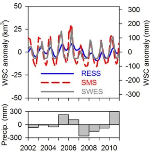
Figure 4. Surface water reservoir storage (RESS), snow water equivalent storage (SWES), and 559
soil moisture storage (SMS) change anomalies for the Sacramento and San Joaquin River 560
basins. Note large reduction in water storages in response to the 2006 through 2009 drought, 561
particularly in the first year of the drought. The precipitation anomaly is based on gridded data 562
from PRISM (Daly et al., 2009). 563
565
566
Figure 5. Groundwater storage (GWS) change anomaly from GRGS data and monthly changes 567
GWS from well data from the upper unconfined aquifer. GWS change anomalies for CSR and 568
GRGS data are shown in Auxiliary Material, Section 4, Fig. S3. A Butterworth filter for removal 569
of seasonal trends and high frequency noise is shown. Application of other filters is shown in 570
Auxiliary Material, Section 3, Fig. S2. Depletion during the drought (31.0±3.0 km3) is shown from 571
Oct. 2006 through March 2010. The precipitation anomaly is based on gridded data from PRISM 572
(Daly et al., 2009). 573
574
Figure 6 . Variations in specific yield from Faunt (2009). 575
576 577
578
Figure 7. Comparison of GWS changes from well analysis relative to simulated GWS changes 579
from the Central Valley hydrologic model (CVHM; Faunt, 2009). Drought periods are shaded 580
(1976 – 1977; 1987 – 1992; and 2006 – 2009). 581
Table 1. Trends in groundwater storage (GWS) changes during the drought in mm/yr, km3/yr, 583
and in total km3 for the different time periods shown based on GRGS and CSR GRACE data 584
and well data (920 wells from the monitoring network). Depletion trends for different time 585
periods and associated standard errors were estimated using weighted linear least squares 586
regression, considering the inverse of squared errors (monthly for CSR and 10 d for GRGS) in 587
the weighting process. Oct 1 2006 through Mar 31, 2010 represents the maximum depletion of 588
GWS during the drought (Fig. ). Trends from Apr 1 2006 – Mar 31 2010 were calculated for 589
comparison with depletion estimates from Famiglietti et al. (2011). Trends from Apr 1 2006 – 590
Sep 30 2009 were calculated to compare depletion estimates from GRACE with those from 591
analysis of 920 wells (Fig. 5). Results from application of different filters to remove seasonal 592
fluctuations and high frequency noise are provided, including Butterworth, centered 12 month 593
moving average (MA), a six-term harmonic series (sine and cosine periodic waves with annual, 594
semiannual, and 3-month periods) (Seas.), and no temporal filter (trend from raw data). 595
Time Interval Model Filter Trend (mm/a) Error (mm/a) Trend (km3/a) Error (km3/a) Volume (km3) Error (km3) Oct 1, 2006 to Mar 31, 2010 GRGS Butterworth 57.6 5.5 8.9 0.8 31.0 3.0 Moving average 58.1 5.6 8.9 0.9 31.3 3.0 Seasonal 57.8 9.2 8.9 1.4 31.2 5.0 None 9.4 - 1.4 - 5.1 - Apr 1, 2006 to Mar 31, 2010 GRGS Butterworth 55.9 5.3 8.6 0.8 34.4 3.3 CSR Butterworth 44.9 8.5 6.9 1.3 27.7 5.2 Apr 1, 2006 to Sep 30, 2009 GRGS Butterworth 49.9 4.8 7.7 0.7 26.9 2.6 Wells Butterworth 49.7 0.5 7.7 0.1 26.8 0.3 596 597