Development of a Three-Dimensional Camera Based on
Subsampled Optical Coherence Tomography (OCT)
by
Meena Siddiqui
M.S. Electrical Engineering and Computer Science, MIT (2013)
B.S., Bioengineering, UC-San Diego (2009)
Submitted to the Harvard-MIT Division of Health Sciences & Technology
in partial fulfillment of the requirements for the degree of
Doctor of Philosophy in Medical Engineering and Medical Physics
at the
MASSACHUSETTS INSTITUTE OF TECHNOLOGY
September 2015
I
@
Massachusetts Institute of Technology 2015. All rights reserved.
Author...
Certified
c 'CD C C~~ C, co Vn ~jR*
Signature redacted
HarvarV-MIT Dvision of Health Sciences & Technology August 28, 2015
by
Signature redacted
Benjamin J. Vakoc, PhD
Associate Professor of Dermatology and Health Sciences & Technology
Siqnature redacted
Thesis Supervisor
Accepted by...
.
...
Emery N. Brown MD, PhD
Director,
arvard-MIT Program in Health Sciences & Technology
Professor of Computational Neuroscience and Health Sciences & Technology
MITLibraries
77 Massachusetts Avenue Cambridge, MA 02139 http://Iibraries.mit.edu/ask
DISCLAIMER NOTICE
Due to the condition of the original material, there are unavoidable flaws in this reproduction. We have made every effort possible to provide you with the best copy available.
Thank you.
The images contained in this document are of the best quality available.
Development of a Three-Dimensional Camera Based on
Subsampled Optical Coherence Tomography (OCT)
by
Meena Siddiqui
Submitted to the Harvard-MIT Division of Health Sciences & Technology on August 28, 2015, in partial fulfillment of the
requirements for the degree of
Doctor of Philosophy in Medical Engineering and Medical Physics
Abstract
Optical coherence tomography (OCT) allows label-free, three-dimensional imaging of tis-sue structure. Current implementations of OCT can either image over long depth ranges at slow imaging speeds, or over limited depth ranges at high speeds. Here, we describe a new OCT paradigm that supports simultaneous high speed and long depth range imaging through subsampling bandwidth compression. We show that this requires replacing the conventional wavelength-swept OCT laser source with a wavelength-stepped laser. First we validated this concept by modifying a slow, conventional wavelength-swept source with an intra-cavity Fabry-Perot etalon to provide a wavelength-stepped output. Using this source in an existing OCT system, we show that we can passively compress signals across a large depth range into a limited RF bandwidth. Next, to demonstrate high-speed op-tical domain subsampled imaging, we developed a novel wavelength-stepped laser source based on intra-cavity pulse compression/stretching; this source provided an A-line rate of ~19 MHz. We then built a polarization-based quadrature interferometer to remove imaging artifacts induced by subsampling and comple-conjugate ambiguity. A calibration and error compensation method was developed to fully remove residual artifacts in the image. We combined the high speed laser and the interferometer to demonstrate the first OCT camera-like imaging across several centimeters of depth range. The optically subsampled OCT technology developed in this work may offer a new three-dimensional camera platform for endoscopic and intraoperative imaging applications.
Thesis Supervisor: Benjamin J. Vakoc, PhD
Acknowledgments
This thesis has been possible due to immeasurable support from my supervisor Dr. Ben-jamin J. VAKOC. I am truly grateful for his mentorship and for the opportunity to work with him and learn from him. I also appreciate his patience with me as I explored a new field. I would like to thank Dr. Elfar ADALSTEINSSON for serving as the chair of my committee. His guidance and support was extremely valuable in navigating the final years of my PhD. I am inspired by his immense knowledge and I will remember his valuable advice for the rest of my career. My thanks also goes to Dr. Guillermo J. TEARNEY for serving as my committee member and thesis reader. His vast insight on OCT technology and his clinical perspective were invaluable during the final stages of this work. And finally, a sincere thanks to Dr. Anantha CHANDRAKASAN who oversaw the production of my MS thesis in the EECS Department.
I am grateful for the company and help from my fellow lab mates and colleagues over the years. I would like to acknowledge Dr. Serhat TOZBURUN for his contributions to the high-speed dispersion-based laser. A special thank you to my colleague and friend Dr. Norman LIPPOK for his mentorship in the last year of my PhD, and for being a willing volunteer for imaging. Thanks to Ahhyun Stephanie NAM and Dr. Ellen Ziyi ZHANG
for enduring the full duration of the thesis with me, and for many stimulating discussions. I have also had many insightful conversations and lunches with: Dr. Nishant MOHAN, Dr. Isabel CHICO-CALERO, Hongying TANG, and Jonathan WELT, Petronella BODO, and Ashley FLIBOTTE.
This journey would not have been the same without my friends and the many hikes, climbing excursions, ski trips, picnics, get-togethers, gym days, and endless adventures we've had. They were an integral part of my PhD life and my happiness/well-being. A special thank you to Dr. Alexander J. NICHOLS for his support and kindness, and for introducing me to the east coast winters.
Above all I would like to thank my family for their unconditional love and support. I am grateful to have my siblings, Hadia SIDDIQUI, Harris A. SIDDIQUI, Edrees M. SIDDIQUI, and Faria M. SIDDIQUI. I have shared so many happy moments with them, and with my little niece, Sophia BADIHI. Thanks to my aunt, Mina M. Sara, for al-ways thinking of me and sending care packages. And finally, with my deepest love and gratitude, I thank my parents Hafizullah K. SIDDIQUI and Soraya SIDDIQUI for always believing in me.
I would like to acknowledge the following organizations for their generous support: National Science Foundation - Graduate Research Fellowships Program (NSF-GRFP) Harvard-MIT Health Sciences & Technology and NIH - SHBT Training Grant
Wellman Center for Photomedicine - Graduate Scholarship Thanassis and Marina Martinos - Medical Imaging Scholarship
6
-Contents
1 Introduction
1.1 Applications of OCT . . . . 1.2 Practical limitations of OCT . . . . 1.2.1 Long-Range Imaging . . . . 1.2.2 High-Speed Imaging . . . .
1.2.3 Acquisition Bandwidth Limitation .
1.3 Thesis Organization . . . . 11 11 14 15 17 18 20
2 Fundamental Concepts in OCT 23
2.1 Monochromatic interference ... ... 23
2.2 Time-domain OCT (TD-OCT) . . . 26
2.2.1 Correlation functions . . . 26
2.2.2 Gaussian sources . . . 29
2.2.3 Low-coherence interferometry . . . 30
2.3 Fourier-Domain OCT . . . 33
2.3.1 Swept-source OCT (SS-OCT) . . . 36
2.3.2 Sensitivity advantage over TD-OCT . . . 38
2.3.3 Balanced Detection . . . 42
2.4 Practical considerations and limitations of FD-OCT . . . 43
2.4.1 Coherence Length . . . 45
2.4.2 Discrete sampling with acquisition card . . . 46
2.4.3 Complex-conjugate ambiguity . . . 49
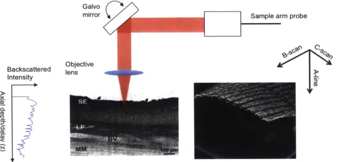
2.5 Transverse scanning and microscopy . . . 51
3 Theory of Discrete Optical Sampling
3.1 Sparsity in Extended Depth Range OCT . . . .
3.2 Bandpass Sampling . . . .
3.2.1 Electrical-Domain Subsampling . . . .
3.2.2 Optical-Domain Subsampling . . . .
3.3 Subsampled OCT imaging parameters . . . .
3.4 Complex-conjugate ambiguity in subsampled OCT.
55 55 57 58 60 64 68
4 Experimental Validation of Subsampling in a Slow-Speed System
4.1 Relevant W ork . . .. .. .. . .. .... . .. . . . .
4.1.1 Polygon-based wavelength-swept laser ... 4.2 Fabry-Perot comb filter ...
4.3 Laser construction and performance . . . . 4.3.1 Coherence length . . . . 4.3.2 Chirp and nonlinear tuning . . . . 4.4 Interferometer and acquisition . . . . 4.5 Experimental validation of circular wrapping . . . ...
4.5.1 Signal loss due to higher order harmonics . . . . 4.6 Experimental validation of imaging . . . . 4.6.1 Im age Processing . . . . 4.6.2 Finger and phantom imaging . . . . 5 Novel High-Speed Subsampled Laser
5.1 Relevant work . . . .
5.2 Laser operating principle . . . .
5.2.1 Dispersion compensation . . . .
5.3 Practical considerations . . . . 5.3.1 Intensity modulator pulse synchronization . . . .
5.3.2 Polarization-mode dispersion . . . . 5.4 Laser Perform ance . . . . 5.4.1 Subsampled operation . . . . 5.4.2 Continuously-swept operation . . . . 5.4.3 Coherence length measurements . . . . 5.4.4 Future laser modifications . . . .
71 . . . . 71 . . . . 72 74 . . . . 76 . . . . 77 . . . . 77 . . . . 79 . . . . 82 . . . . 84 . . . . 86 . . . . 87 . . . . 89 93 . . . . 93 . . . . 94 . . . . 97 . . . . 100 . . . . 100 . . . . 100 . . . . 100 . . . . 100 . . . . 103 . . . . 104 . . . . 107
6 High-Extinction Complex-Conjugate Ambiguity Removal 6.1 Introduction . . . . 6.2 Experimental system design . . . . 6.2.1 Polarization-based demodulation circuit . . . . 6.2.2 OCT system . . . . 6.3 Mathematical framework describing errors and error-correction optical quadrature demodulation circuits . . . . 6.4 Calibrating the optical demodulation circuit . . . . 6.4.1 Coherent fringe averaging . . . . 6.4.2 Correcting only spectral errors . . . . 6.4.3 Correcting both spectral and RF errors . . . . 6.5 Stability analysis . . . . 6.6 Im aging . . . .. . . . . 6.7 Discussion . . . . 109 109 111 111 113 in passive . . . 114 . . . 116 . . . 117 . . . 118 . . . 120 . . . 123 . . . 125 . . . 126 8
7 3D Camera Imaging 129
7.1 Hardware system integration . . . 129
7.1.1 Acquisition configuration . . . 130
7.1.2 Microscope . . . 132
7.2 Performance characterization . . . 133
7.2.1 Coherent averaging . . . 135
7.3 Image processing . . . 136
7.3.1 Complex conjugate demodulation in subsampled imaging . . . 136
7.3.2 Dispersion removal . . . 139
7.4 Imaging . . . 141
Chapter 1
Introduction
1.1
Applications of OCT
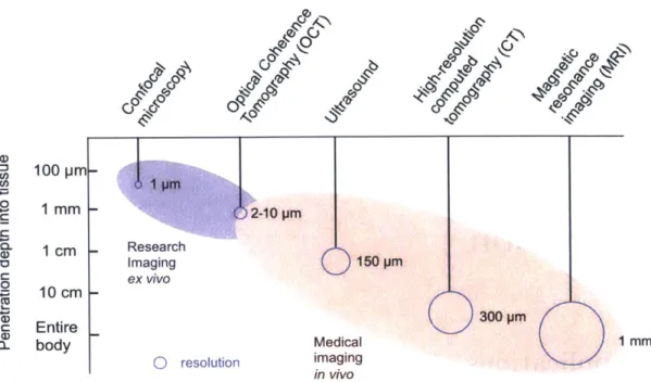
Optical coherence tomography (OCT) is a high-resolution, three-dimensional imaging modality that uses infrared light to probe depths within tissues [15, 441. For many appli-cations, OCT is advantageous because it offers a resolution and penetration depth that is not achievable by other modalities. Figure 1-1 shows a comparison of various imag-ing techniques. Confocal microscopy provides the highest resolution, however it is used primarily as a research tool because of its limited penetration into tissue and because of the challenges associated with implementing it clinically. On the other hand, technologies like ultrasound, CT, and MRI have low spatial resolutions in standard clinical practice and cannot visualize the microstructure of tissues. With a resolution on the order of a few pm, and a penetration depth on the order of 1-2 mm in highly scattering tissues (i.e. skin, GI tissue), OCT offers a new medical diagnostic and disease monitoring technique. The contrast in OCT is provided by intrinsic variations in tissue scattering based on inho-mogeneous optical index of refraction and therefore does not require exogenous contrast agents. This enables non-invasive three-dimensional visualization of tissue morphology as well as depth-resolved functional imaging. OCT is often compared to histology because it is on a similar size-scale and in fact one of the original goals of this technology was to perform optical biopsy
1451.
1o 00-Q-0p mm 1 cm - Research Imaging U 150 PM ex vivo 0 10 cm 300 pm c Entire 0- body Medical 1mm b resolution imaging in vivo
Figure 1-1: A schematic comparison of OCT and other imaging modalities based on resolution, penetration depth, and clinical utility.
The earliest time-domain OCT systems (TD-OCT) focused on applications in
ophthal-mology [15]. In 1993, the first in vivo tomograms of the human optic disc and macula
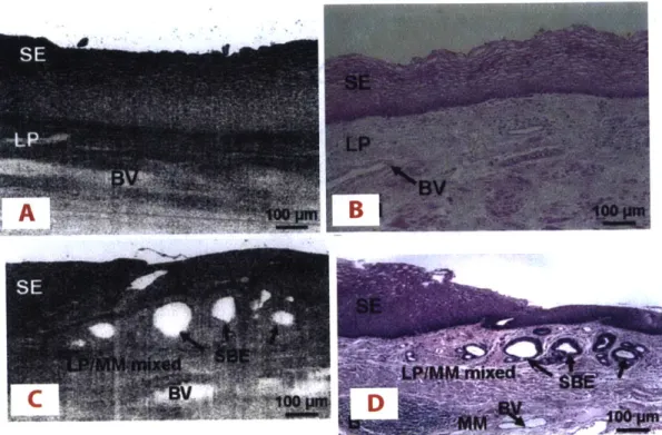
were demonstrated [411. With extensive research effort over the following decade, longer wavelengths and higher power lasers gave rise to imaging of optically scattering and non-transparent tissues [4]. Ex vivo investigation of OCT was conducted in a variety of organ systems including cartilage, gastrointestinal tissues, upper respiratory tract, and and uro-logic tissues [4,19,36,37,44,45]. All of these studies showed that OCT has strong clinical potential for a wide range of diseases and organ systems. In epithelial cancers, for in-stance, disruption of cellular organization beneath the surface of the tissue can provide indicators of dysplasia. Figure 1-2A is an OCT image of a segment of normal human esophagus, with Figure 1-2B showing the corresponding histology. In this health tissue, the organized structure of the tissue layers is apparent in the OCT image, and this or-ganization is disrupted in the case of sub-squamous Barrett's epithelium as shown in the
Figure 1-2: Representative OCT images of human esophagus and corresponding histology.
A & B) Normal esophagus with squamous epithelium (SE), lamina propria (LP), and
mus-cularis mucosa (MM) are clearly visible on the OCT image. C & D) Barrett's esophagus with disrupted architecture and multiple subsquamous Barrett's epithelial (SBE) glands beneath the SE are visible on both histology and OCT image
[7].
OCT and histology images of panel C and D
17].
Evidently, this technology can have ahuge impact on the standard-of-care for disease screening, monitoring, and treatment.
In recent years, advancements in functional OCT have further broadened the potential for OCT to make a clinical impact. Angiographic OCT, for example, has been used to visualize flow in many systems including retina vasculature, skin vasculature, and tumor models
[24,51,62].
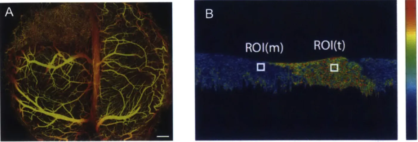
There have been several algorithms used to perform angiographic OCT including Doppler methods and speckle decorrelation methods 127]. Figure 1-3A shows an image of a tumor micro-vasculature in a mouse brain imaged with a Doppler OCT al-gorithm. Polarization-sensitive OCT (PS-OCT) is another functional OCT method that adds contrast for tissue composition. It detects the depth-dependent changes in thepo-Figure 1-3: A) OCT angiography projection of vasculature in a mouse brain with a glioblastoma tumor (Scale: 500 pm)
1511.
B) OCT generated birefringence map of chicken muscle (ROI(m)) and tendon (ROI(t)). Colorbar: 0-2 deg/pm [611.larization state of light through a sample; Figure 1-3B is an example of a PS-OCT image showing the local birefringence of tendon/muscle junction [61].
1.2
Practical limitations of OCT
Since OCT is based on fiber optics, it can be incorporated into many existing in vivo imaging modules, i.e. endoscopes. Initially, however, clinical imaging was only performed on external organ systems that were easy to access such as the skin, oral cavity, and eye. With the introduction of catheter-based fiber optic probes around 1997, imaging of internal organs first became possible
[451.
These initial systems were limited in their utility due to a combination of small imaging fields, motion artifacts, and difficulty meeting geometric constraints in the organs. The potential of in vivo imaging drove research efforts in following years to focus on: 1) longer imaging ranges that reduce sensitivity roll-off due to organ geometry[33],
and 2) higher speed laser sources that enable real-time image rendering and minimize motion artifacts [17,28, 421. Although some improvements have been made in these areas individually, it is the combination of high-speed and long-range imaging that enables wide-field, camera-like imaging with OCT.Sd&VbW Famaimod SW Balm ale ca P W C
Figure 1-4: Top: A balloon catheter centration mechanism that allows for circumferential imaging of the esophagus. Botton: Physical implementation of the balloon probe [521.
1.2.1
Long-Range Imaging
The first generation TD-OCT systems relied on a translating reference arm for depth scanning. However TD-OCT was impractical for clinical imaging because of slow imaging speeds and low sensitivity. Consequently, motion artifacts were severe and imaging could only reliably be performed on small volumes
[15,
19, 361. The introduction of Fourier-domain OCT (FD-OCT) obviated the need for a translating reference arm and instead relied on the laser source for imaging speed. In these systems, however, the coherence length, or length over which light in a sample arm is well correlated with light in a reference arm became a relevant parameter in determining the imaging range [46,59].
Until some recent advances in swept laser technology, the limited coherence length of OCT lasers required tight control of the distance between the imaging probe and the tissue surface.If the tissue was located more than a few millimeters from its ideal location, the OCT
system rapidly lost its sensitivity and the tissue could not be imaged. For this reason, existing clinical applications of OCT use careful engineering to meet this low depth range criteria. In endoscopic OCT, for example, the smooth and tubular nature of the organ
(b) duodenum
Figure 1-5: (a) Endoscopic OCT image of esophagus obtained with a balloon catheter.
G = gland, MM = muscularis mucosa; (b) Analogous image of the duodenum where
comprehensive imaging is difficult because of villi and uneven surfaces
[401.
allows imaging through a balloon-centration catheter, which arranges the tissue within the coherence length with millimeter-level accuracy (Figure 1-4)
[52].
Organs with more complex geometries, or clinical applications that require wide-field imaging cannot be accommodated. For instance, because tissue along the intestines are have irregular crypts and varying diameters at different sections, balloon catheterization is not as effective in centering the imaging probe. Figure 1-5b shows a cross-section of the duodenum that is imaged with the same balloon catheter as in the esophagus. The left side of the duodenum has fallen beyond the imaging range of the system and these re-gions are potentially missed during screening of disease. If the imaging probe is moved to visualize the left region of the duodenum, the right edge is out of the field-of-view (FOV). This example demonstrates the difficulty of achieving comprehensive imaging without longer imaging ranges. Until now, the limited capability to acquire long-range signals has slowed efforts to explore long range laser sources, however some recent lasers have demon-strated multi-cm scale coherence lengths
[33,391.
As more sources are demonstrated with these capabilities, new clinical and industrial applications of OCT based on simultaneous high-speed and multi-cm depth ranges can be envisioned.16
B
Figure 1-6: A) A longitudinal cross-sectional image of a tissue with arrows pointing to location of motion artifacts. B) A three-dimensional rendering of the esophagus image
showing severe motion artificts in the left section 152].
1.2.2
High-Speed Imaging
High-speed imaging is important for minimizing motion artifacts during the imaging ses-sion, as well as for real-time image rendering. Most tissues in the body do not remain stable for prolonged periods of time, and are subject to various motions, whether from breathing, heart beating, peristalsis, or other biological functions. Significant motion of the tissue relative to the imaging probe within this time induces artifacts in the image that are difficult to remove in the processing stage Figure 1-6a). To minimize these ar-tifacts, tissue must be immobilized for the duration of the imaging session; while this is straightforward in external tissues, it poses a larger challenge in internal organs. In the esophagus, the aforementioned balloon catheter provides limits motion during the imaging procedure, however, some motion is unavoidable even in these applications (Fig-ure 1-6b) [52]. Furthermore, stabilization via a balloon catheter cannot be applied to many other internal organs, and as such motion artifacts are prohibitively large.
In OCT, the A-line rate (given in Hz) is the number of axial scans that can be
Table 1.1: Approximate OCT Imaging Times for Various Volumes A-line Rate 1cm x 1cm x 2mm 5cm x 5cm x 2mm 1 kHz 1.1 hours 27 hours 100 kHz 6 mins 2.7 hours 1 MHz 4 s 1.7 mins 10 MHz 0.4s 10 s 20 MHz 0.2 s 5 s
and thus less motion can occur during that interval. Table 1.1 provides some exemplary values for the time it takes to acquire a 1cm x 1cm x 2mm or a 5cm x 5cm x 2mm volume with different A-line rates. Realistically, in vivo imaging should be performed in a fraction of a second since cardiac motion occurs on the order of once per second. In 2004, swept-wavelength OCT imaging was demonstrated at 10 kHz A-line rates [57]. Since then, multiple new swept-wavelength technologies have been developed and laser speeds have increased to the order of MHz [17,31]. With this increase in speed, in vivo imaging is becoming easier and more informative.
1.2.3
Acquisition Bandwidth Limitation
In standard Fourier-domain OCT (FD-OCT), the frequency of the signal you must ac-quire scales linearly with how far away you tissue is from your imaging probe. It also scales linearly with how fast you image, thus when the requirements of high-speed are combined with those of extended depth range imaging, current acquisition electronics are unable to accommodate the resulting signal bandwidth. Figure 1-7 is a schematic of the physical depth space (top) and the corresponding RF space that maps the OCT signal (bottom). In this example, assuming a 20 MHz Aline rate (high-speed laser), a tissue ap-proximately spanning the physical space of 3.7 mm - 4.3 mm results in an RF bandwidth approximately spanning 9.75 GHz - 10.25 GHz. This RF signal is well beyond what we
are able to acquire with modern digitizers and because of this we are currently limited by the acquisition bandwidth this limits the depth range over which we can image our tissue.
mm 2mm 4mm mm 8MM depth OCT b~ co (D 0 0 GHz I 5 GHz 10 GHz RF Bandwidth
Figure 1-7: Top: A schematic of tissue placed at a 4 mm depth away from the imaging probe. Bottom: The corresponding tissue signal in the RF bandwidth based on simulated tissue signal spanning a 1 GHz range. The grey shaded area is not acquirable by current
acquisition electronics.
15 GHz 20 GHz
Tissue Attenuated tissue Air/saline
In this work, we demonstrate a method to dramatically reduce the acquisition band-width required for extended depth range imaging, thereby enabling high-speed and long depth range OCT with current acquisition electronics. Notice in Figure 1-7 that although the tissue signal occupies a high RF frequency space, the bandwidth of the tissue signal occupies a small region of the total RF bandwidth. This is because the penetration depth of light into tissue (referring to how far into the tissue light travels) is much smaller than the depth range of imaging. This penetration depth depends on the wavelength of the light, the output power of the light source, the sensitivity of the imaging system, and the scattering of the tissue. Typically for highly scattering tissues such as skin or esophagus, penetration depths are ~2-3 mm. In this work we take advantage of the sparsity in the RF space to compress the tissue signal into a lower baseband frequency. Our approach is based on modifying the optical sampling approach in OCT so that wavelengths are dis-cretely instead of continuously sampled. With this subsampling method, the acquisition bandwidth is no longer limiting the depth range, and we can acquire tissues along the entire coherence length of the source.
1.3
Thesis Organization
The goal of this work is to create a new platform technology that enables three-dimensional camera-like imaging with OCT. This requires fundamental changes to the laser, interfer-ometer, and signal processing, so that long-range, high-speed, and wide-field imaging can be performed with minimized acquisition bandwidths. Chapter 2 describes the funda-mental background of OCT and section 2.4 focuses salient concepts that were utilized extensively in this work. Chapter 3 introduces the theory behind incorporating optical subsampling into OCT, and makes the connection between subsampling parameters and standard imaging parameters. Chapter 4 describes our proof-of-concept set-up and our experience with the first subsampled imaging system. Chapter 5 describes the design and performance of our novel high-speed dispersion-based subsampled laser. Chapter 6 describes how we removed complex-conjugate artifacts in our images by developing a
new method of high-extinction quadrature interferometry. In Chapter 7, we integrate the subsampling concept, our novel dispersion-based laser, and our novel quadrature interfer-ometer to acquire unprecedented wide-field images with our camera-like OCT system.
Chapter 2
Fundamental Concepts in OCT
The fundamental structure of OCT systems consists of three major components: a light source, an interferometer, and a data acquisition/processing unit. At the core of OCT theory is the concept of light interferometry. This chapter begins by introducing the concept of interferometry in the context of time-domain OCT (TD-OCT). The evolution of OCT into the Fourier-domain is then described as well as some prevailing concepts that this work builds upon.
2.1
Monochromatic interference
Although monochromatic plane waves are never found in nature, they provides a good model for studying phenomenon like light interference. In OCT, the Michelson interfer-ometer is employed as an essential tool to indirectly measure backscattered light from different depths within a sample. The light is otherwise traveling too fast for photode-tectors to acquire. A common schematic of this interferometer is shown in Figure 2-1.
I
Light that is generated from a laser source enters the beam splitter (BS) and is divided into the reference arm and the sample arm. The light that is backreflected from each arm recombines at the beam splitter and the interference of these two beams is received
by a photodetector. Assuming that the monochromatic source has a wavenumber k0,
reference E Z ER ZR AZ=Z -Zs BS laser D --- ---E= ER + E PetorI
Figure 2-1: A schematic of a simple Michelson interferometer where the single-pass
refer-ence arm distance is ZR and the sample arm is zs.
zs respectively, the complex electric field amplitude of the light in the reference arm is
R(z) EReikozR and in the sample arm Es(z) = Esejkozs. When the light recombines
at the beam splitter the total electric field is the superposition of these electric fields (following the linearity of the Helmholtz equation) [13]:
ET(z) = ERe 2jkZR + Es .2kozs (2.1) The factor of 2 results from the double-pass travel in each arm of the interferometer. For simplicity, the amplitude changes and phase delays induced by the components in the optical beam path are ignored. Because photodetectors detect the irradiance (energy per unit area per unit time) rather the the electric field, the interference is expressed in terms of average intensity
[131,
I =(_E z2
(2.2)
= IR + Is + 2 IKIs cos(2k, A z)) 24
where
()T
denotes time average over time T, which is chosen to be much longer than an optical period. AZz = z- zS refers to the optical path difference between the sample and the reference arm as shown in Figure 2-1. Thus the intensity of the total electric field at the detector is a sum of time-independent and depth-independent DC terms and an interference term that sinusoidally varies with path length differences. The latter term forms the basis of backscattered light detection in OCT.This equation makes sense intuitively because varying the optical path difference Az causes the sample and reference arm waves to alternatively constructively and destruc-tively interfere with each other. The average intensity does not vary with time, and this is also true for stationary polychromatic waves as we will see later [5,131. Note that in this
case of monochromatic light, the wavenumber can equivalently be expressed as ko = o and the time it takes for the light to travel a distance ZR is given by tR = ZRa and simi-larly for the sample arm, ts = zsg. When considering low-coherence light, the properties
of the material through which light propagates becomes important in determining the dispersion relation. Hence,
TC
Az = (2.3)
where r tR - ts represents the time difference of travel between the two reflectors. Thus the intensity can also be expressed as
[5],
I IR+ Is + 2IR 1
S cos(2w0 T)) (2.4)
This provides a more convenient representation when describing polychromatic or low coherence waves in following sections. Interestingly the DC terms also represent an in-terference, however because it is the interference of reference and sample arm light with itself, it is always constructively interfering because Az = r = 0.
If the reference mirror were scanned back and forth in time, Az(t), then the interfer-ence oscillations can be detected with a photodetector, which converts the irradiance to
an analog current based on the following:
14,51,
idet(T(t))= p[ PR + PS + 2 PRPS cos(2wr (t))] (2.5)
where p = q is the responsivity of the detector
(units
Amperes/Watt), r is the quan-tum efficiency of the detector, q is the quanquan-tum electric charge (1.6 x 10- 19C), and hVis the photon energy. PR and Ps are the powers detected by each reflector in the sam-ple/reference arm and are proportional to IR and Is multiplied by the receiving area of the photodetector. Notice that the amplitude of the signal is proportional to the product of the magnitude of the reference and sample electric fields, implying that a weak backscat-tered field from the sample can be amplified by mixing with a strong reference field. In this hypothetical monochromatic case, the interference oscillations will be observed for infinitely wide path differences (Figure 2-2a), which has limited utility in OCT since we are interested in measuring intensity at a particular location in the sample field. This is why broadband light sources that produce low-coherent light are used.
2.2
Time-domain OCT (TD-OCT)
2.2.1
Correlation functions
Low-coherence or broadband polychromatic light cannot be assumed to be a time-independent deterministic complex function; a randomness is introduced, which gives the wave function a dependence on time and position and requires statistical methods to describe. First, we can think of polychromatic light as a superposition of monochromatic waves. Since the wave equations are homogeneous linear partial differential equations, any linear combina-tion of a solucombina-tion is also a solucombina-tion. The complex wave equacombina-tion can thus be expressed as a Fourier integral,
E(z, t)
j
Eo(z, w)eil3zeiwtdw (2.6)(b)
-M
Infinite coherence length
-- + +-- AIFWHM
At
Finite coherence length
Figure 2-2: (a) Interference fringe resulting from a source with infinitely long coherence length. (b) Interference fringe resulting from a source with a short coherence length.
where -w and +w are the lower and upper limits of the spectral bandwidth, Aw, and # is the propagation constant defined as:
(w) = n(w)- =k(w) (2.7)
In the case of monochromatic light, there was only one frequency, wO so that O(w) = nr(wo)w0/c = k,. This more general representation accounts for propagation through
dis-persive materials where the index of refraction is frequency-dependent.
As before, the intensity of light is given by the absolute square of the complex wave function, however, for broadband light E(z, t) is a function of time as well, (E(z, t) 2). Its instantaneous intensity is random and the average intensity must be taken
[13,34]:
I(z) - ( E(z, t)I2) (2.8)
where (-) represents the ensemble average over many realization of the random function. Assuming that the partially coherent waves in OCT are stationary, meaning that the average intensity is constant over time, this intensity becomes a function of position only,
1(z). Referring again to the Michelsoni interferometer of Figure 2-1, if a reference arm has
depth of ZR and a sample arm depth of zS, the mutual coherence or correlation function is given by:
g(zR, zs, 7) = (_E*(zR, t)E(zs, t + T)) (2.9)
where r = (ZR - ZS)/C is the double-pass time delay. Since we are evaluating this function at a fixed ZR and zS the simplified correlation function is written as:
gRS(T) = (E (t)Es(t + T)) (2.10)
where gRR(T) = (ER(t)*ER(t + T)) is the case of autocorrelation, which in the case of T = 0 reduces to intensity IR and similarly Is for the sample arm. After normalizing
gRs(T) we arrive at the complex degree of coherence or normalized correlation function:
~RS(T) = 9RS RT gRs(T)
V gRR (0) gss() V"I (2.11)
Recall from Eqn. 2.8 that we have assumed a stationary wave, and since we are evaluating at a particular depth, we have dropped the z-dependence for convenience. Notice that
Jgj(-r)j is the normalized shape of the correlation function and does not account for the
magnitude of intensity of light in the system
[34].
Instead the magnitude of intensity coming from the source, and the fraction of it that reflects back from the reference and sample arms are combined in the terms IR and Is.In the case of autocorrelation of deterministic and monochromatic light, jj(T) = exp(iwor)
so that gi (r)j, the degree of correlation = 1 for all T. However if light is not monochro-matic, gii(T) I drops to a value of 1/e at a delay, Tc or the coherence time. The coherence time is related to the coherence length through the relation:
Ale = -c (2.12)
n
In OCT, this length is a very important characteristic as it directly relates to the axial resolution of the imaging system [10, 34]. In the next section we will establish that the
coherence length relates to the spectral bandwidth and shape of the light source.
2.2.2
Gaussian sources
We established the intuition that monochromatic light is always perfectly correlated, thus
r, = oc. Hence we can imagine that the more polychromatic our light becomes, the
faster it becomes uncorrelated and r, is smaller (portrayed in Figure 2-2b). The Weiner-Khinchin theorem formally establishes this relationship, saying that the autocorrelation of a stationary random process is related to the power spectral density, S(w) through a Fourier transform relationship:
S(W) = g(T)e-wdr (2.13)
S(w) is the average power per unit area per frequency (W/cm2-Hz), or average intensity
per frequency. This implies that the wider the source bandwidth (most commonly defined
by its full-width-half-maximum, FWHM, value), the narrower the autocorrelation. And
the shape of g(r) is determined by the shape of the power spectral density. In OCT, ideal broadband sources have Gaussian shaped power spectrum,
1 (P - WO) 2
S(
- wo)x exp[- (2.14)or 27 2o.2
where I S(w - wo) is the normalized shape of the spectrum. The source FWHM bandwidth is given by w = 2a/ 2 1n2. This yields a correlation function that is also has a Gaussian shape:
1
r
() exp(- ) (2.15)
o7, V2 -7 2a;
where I (T)j is the shape of the correlation function and a, is the standard deviation of Gaussian envelope. The FWHM of
|(T)
I as a function of coherence time of the light source is given bym,
= 2ou/2 1n2. Using that oxax = 1 we arrive at a relationshipbetween coherence time and spectral width Tc = 2 "2 for Gaussian sources. The axial resolution, 6z, of double-pass light path through the sample is !Al,, leading to the axial
resolution expression:
41n2 c _21n2 A22.6
6z n Aw 0 (2.16)
irn AA
where A0 is the center wavelength, AA is the spectral bandwidth and n is the refractive index of the sample [4]. Therefore, it is clear that in order to have high axial resolutions,
OCT sources must have high spectral bandwidths. It is noteworthy that sometimes the
power spectral density function has more of a rectangular shape, and in this case the axial resolution can be calculated by 6z = A2/(2nAA)
f5,10,341.
2.2.3
Low-coherence interferometry
Interference with single sample reflector
As in the monochromatic case, we derive the intensity of the interference of two partially coherence waves:
I(T) =(ER(t ) + Es(t + T)12) (2.17)
IR + Is + 2VIRIS gRS(T)j Cos(pRS(r))
where p(T) = arg{Rs(T) -- aRS(T) - wr and where again w, is the center frequency of the spectrum and aRS(T) is a phase shift that is independent of frequency. Notice that the intensity is directly related to the correlation function, g(T), and the normalized
correla-tion funccorrela-tion, g(T), and the interferogram is a harmonic funccorrela-tion with a frequency that is proportional to the center frequency of the optical broadband spectrum. If qRs(T)I = 1
for all T we have the case of monochromatic light and we arrive at Eqn. 2.4. If gSRs(T)I = 0
we have completely incoherent light, and if 0 < J Rs() 1 < 1 the light is partially coherent and IgRs(T) itself represents the degree ofaoherence. As stated before, the r which causes
IRs(-r) ; 1/e is the coherence time, T, and is proportional to the OCT axial resolution
Interference with multiple sample reflectors
The interference equation in Eqn. 2.17 was derived with the assumption that there was one reflector in the sample arm, however in tissue there are multiple backscattering positions
zi with time delays ri = (zi - ZR)/c. Each reflector results in a cross-correlation with the reference arm light, as well as a self-correlation from different depths within the sample. In
this multiple backscatter case, we can rewrite the intensity as I(T) = (|ER(t)
+f_+o
E (t+Tj) dril2), where Ej is the wave back-reflected from the sample position zi. The sample
arm light is represented as a continuous sum of backreflected field of light arising from different depths within the sample arm, hence the integral ranging from oc. Following
Eqn. 2.17 we can write the intensity of the interference as a function of time delay:
I(T) = (ER(t) E t + E (t + -)Ej *(t + T2)) dcr
+ f(E(t +Ti)Ej(t + -j)*) + (Ej(t + T)*Ej(t +Tj)) drdT, (2.18)
+ f (ER(t)Ei(t + T )*) ( ER(t)*Ei(t + Ti)) dr
As in the case of a single reflector, the first term accounts for the interference of reference arm with itself and contributes a DC term. The second accounts for the sum of all self-interferences within the the sample reflectors, which arise from the same delay, T within the sample and also only contributes a DC term. The third term refers to the interference of sample reflectors arising from different depths within the sample, only for the case where Tj -Z
mj.
And the last term, of greatest interest in OCT, represents the interference of the sample reflectors with the reference arm light. The meaning of this equation becomes more clear when it is cast in terms of the normalized correlation function, g r):I(r) = gRR(T = 0) + j ii(r = 0) dT,
+ R{gj(w = ri - Tj)} dridrj (2.19)
+ 2 iR{gi(T = i) d-ri
Note that T = Tr - Tj = (zi - zj)/c and represents the time delay between two sample reflectors while ri = (zi - ZR)/c and r = (zj - zR)/c represent delays between sample and
sum of sample and reference autocorrelations, intra-sample cross-correlations, and sample-reference cross-correlations. As in Eqn. 2.17 we will write the final intensity function in terms of the normalized correlation function:
I(T) = IR - Ii di
+
11
123 i - 7j) I cos[aij - wO(T - T )] drid-rj (2.20)+ 2 VIi IR |47i r COS [~iR I - wori ] dri
Here again we see that the cross-correlation functions are modulated by a carrier wave that has a frequency proportional to the center frequency of the light source, w0, and a frequency-independent phase term that is a function of optical path delay, ai (Tr - r) and
aiR(Ti). Recall that the amplitude of the normalized correlation represents the degree of
coherence and 4(ri)I > 1/e only when T < r. This means that an interferogram is only
present at a small depth location equivalent to Al, as per Eqn. 2.12. The rate at which
(-ri)|
Idrops to zero is determined by the shape of the spectral density function S(w) in Eqn. 2.13. In TD-OCT, it is the amplitude of the last term that is proportional to the sample reflectivity at a certain depth location within the sample; lock-in detection at thecarrier wave modulation frequency are frequently used to obtain the reflectivity envelope
of the last term. The reference mirror is translated in order to detect different depths within the sample and create a backscatter map at each point in the sample. Notice that the intra-sample cross-correlation term did not exist as long as we were only considering a single reflector within the sample. However, because of the low backscattering intensity from the sample their interferometric gain, hJj, is often negligible compared to the heterodyne gain, /i=R, of the sample-reference interferogram. Additionally, in TD-OCT there is only a small range where (Tr) I = 0 so the sum of intra-sample cross-correlation
contributions to the third term are smaller, hence this term is often ignored. Assuming a Gaussian source, and assuming that the reference mirror is moved at Tr(t), the detector
current for TD-OCT can be represented as:
idet[ri(t)] oc 2 p -1g(Fi(t)) V/PRPs cos(2wTi(t)) (2.21)
where again p is the responsively of the detector (Ampere/Watt) and PR and Ps are optical powers reflected from the reference and sample (respectively) onto the photodetector.
2.3
Fourier-Domain OCT
The transition from time-domain OCT to Fourier domain (FD-OCT) followed closely from the development of optical frequency domain reflectometry (OFDR). This major techno-logical advancement for OCT imaging gave way to improved detection sensitivity, as well as increased imaging speeds as a translating reference mirror was no longer required [57]. In the frequency domain, full sample depth structure is encoded as a depth-dependent modulation of the broadband light. This follows again from the Weiner-Khinchin Theo-rem (Eqn. 2.13) because it says that the depth profile can be obtained from the Fourier transform of the power spectral density function without the need of changing the optical path length in the reference arm. If we start with the Fourier transform pair:
giR(T) = SiR(w)eir dw (2.22)
and apply it to Eqn. 2.19, express the cross-spectral density as SiR(w) = SiR(w)I
exp[i(aiR(w)-wr)], with aiR(w) W T arg {9iR(W)}, we arrive at the intensity as a function of fre-quency. Although this function is intrinsically complex, we measure only the real part
and thus express it as:
f+00 +00 + O [
I(w) =ISRR(w)l +] S (w)I di
+
I
I
Si (w)Icos
(ai-
w(Ti - T))J dTi dTj+ 2 0SiR(w) cos [(aiR - wi) dTi
(2.23) 33
where again, ri = (zi - zR)/c. Unlike in Eqn. 2.20, where the interferogram had a
modulation that was proportional to the center frequency of the light source, wO, now the interferogram modulation is a function of optical path delay, Tr. Information from all depths are contained within this intensity function, hence the reference arm does not need to be translated. This serves an improvement in sensitivity as we will see later in section 2.3.2. The depth information in the time-domain can be obtained by taking the inverse Fourier transform of Eqn. 2.23,
I(T) F1{I(w)} =gR(0) + gii(0) di
+
f{[Tgij[T+
(Ti - Ti)] +gij[T - (TZ - T3i)] dTidT (2.24)+ 2 {YiR(T - Ti) + giR(T - Ti) dri
This expression is analogous to Eqn. 2.20 in TD-OCT. The first two terms correspond to the unmodulated DC intensities resulting from the reference arm reflection and the sum of back-reflected intensity from all scattering sites within the sample. The third term is the undesired intra-sample cross-correlation contribution; note that in TD-OCT this only resulted from sample scatterers within the coherence time, Tc, however now this term can contain intra-sample cross-correlations from the entire sample depth. Only the sample-reference cross-correlation term in the fourth term contains information about the backscattering coefficient and the sample structure. The correlation function is centered
about the variable r and has a value g(TTry)l ; 1/e only when r tril < . In TD-OCT
the correlation function was always assumed to be centered about zero delay (T = 0) and
the reference arm was moved to scan the sample depth. Now the intensity function in-herently contains information about all depths (within a certain sensitivity roll-off as we will see in section 2.4.1). Also, the intensity signal is symmetric about the zero delay, hence two scatterers located at zi ZR - Az and zi = ZR + Az will result in the same frequency modulation. To avoid this, the sample can be placed such that the surface and entire penetration depth lies on one side of the zero delay. Alternative ways to avoid this
overlap are discussed in Section 2.4.3, and is a major consideration in subsampled imaging.
For convenience, the sample-reference cross-correlation term is often written as a con-volution,
IiR( ()) - SR(W)- IiR (7) - (T) I 0iR (T)' (2.25)
where IS(w)I is the shape of the source spectrum, I'(T)I is the shape of the correlation function (this does not have a dependence on the reflectivities). We have defined
SiR(w)'
as the interference modulation of the spectrum scaled by the sample and reference reflected intensities (IR and Is). And similarly iR(T)' is the Fourier transform ofSiR(W)'
and represents the location and intensity of the reflector at each depth within the sample.I+00
SiR(w)' - VfIRIi - cos(wTi) dTj -2
- (2.26)
giR(T)
j
'RIi [6iR(T + Ti) + 6iR(T - Ti)] dTIR and Is are reference/sample reflectivities, 6
iR is the Dirac delta function, and 0 denotes the convolution. Eqn. 2.25 highlights that the in the time-domain, the signal of a single sample reflector is a delta function with a shift proportional to optical path delay, Ti, an amplitude proportional to the the sample/reference reflectivities, and an axial resolution proportional to the envelope of the correlation function, similar to TD-OCT as was shown in Section 2.2.2.
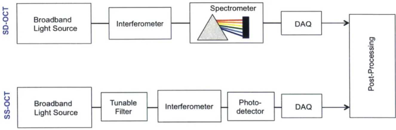
The signal described by Eqn. 2.23 can be obtained either by spectral-domain OCT
(SD-OCT) or by swept-source OCT (SS-(SD-OCT), as depicted in Figure 2-3. The first technique
is to use a continuous wave (cw) broadband light source and detect the spectral compo-nents of the power spectral density function by separating the optical frequencies with a spectrometer at the interferometer output. This technique is termed spectral-domain
OCT (SD-OCT). Another technique is to use a tunable laser with a narrowband linewidth,
where the center wavelength is swept with time over a broadband range (i.e. spanning
I-- Spectrometer
o Broadband Itreoee A
Light Source Interferometer
I--C.).
o Broadband TnbePoo
BrLight Source Filter Interferometer detecr DAQ
Figure 2-3: Schematic of swept-source (SS-OCT) and spectral-domin (SD-OCT) imple-mentations of FD-OCT.
100nm centered at 1550 nm). This is termed swept-source OCT (SS-OCT) and the ad-vantage of it is that the interferogram can be obtained with a single photodetector. The subsampling concept we have introduced in this thesis applies to both SS-OCT and
SD-OCT setups, however, we focused primarily on SS-SD-OCT.
2.3.1
Swept-source OCT (SS-OCT)
In SS-OCT the spectral interferogram is captured sequentially by recording the signal with a single detector while tuning the frequency of a narrowband laser. The detector current can be written as,
idet[W(t)] = P (W(t)) PR, + P I W(t)) IJ+0Pi dri
+ p 5(w(t))
j/fFP
3 -cos[w(t)2(Tr - Tj))] dTidTr (2.27)+ 2p I (w(t)) / PR-i - cos[w(t)2r] dc1T
where again p is the responsivity of the detector and the factor of 2 in the modulation results from the double-path travel of light in the Michelson interferometer. In the simplest case of linear tuning, where w(t) is varied linearly in time with a constant slope a' - dw
(units Hz/s) then w(t) = w0
+
a't where w is the lowest frequency in the spectral profile.Again, the last term is the sample-reference cross-correlation.
idet[w(t)] oc 2pjS(w(t)) P P -cos[2wri + 2Tia't] dTj (2.28)
The frequency of the detector current is directly proportional to the tuning slope and the optical path delay,
2Tri'
fdet = (2.29)
27r
The tuning rate is often expressed in terms of the "A-line rate" (expressed as fA) and
a' = (2.30)
Duty cycle
where /w is the FWHM spectral bandwidth of the source as we referenced in section 2.2.2 for Gaussian sources. Sometimes the duty cycle of swept-sources are not 100% so the Aline rate must be divided by the duty cycle to achieve an "effective A-line rate". The frequency can be rewritten in terms of this rate:
2TrAw -(fA) 2AzAw -(fA) 2AzAA -(fA)
27 (Duty cycle) 27c (Duty cycle) A2(Duty cycle)
where A A is the FWHM spectral bandwidth expressed in wavelength and AO is the center wavelength. Thus it is formally shown that the interference fringe frequency is directly proportional to the A-line rate of the swept source and the depth range that you are imaging over
[10.
Since modern digitizers are limited in bandwidth, simultaneous long range and high speed imaging cannot be performed without compression (Figure 1-7 has already suggested this in section 1.2.3). It is easily shown that for SS-OCT, the sampling interval is related to the fringe frequency, fdet and the digitization frequency, fdig,
Aw fdet (2.32)
where 6w, is the electronic sampling interval induced by digitizing the interference fringe. We will see in section 2.4.2 that if this interval is not small enough, i.e. because the digitization rate is not fast enough, it can limit the depth range of the OCT system.
Nonlinear tuning
We have established that the optical properties of the light source have an impact on imaging parameters like axial resolution. In SS-OCT, it is not only the optical properties of the source that effect the imaging parameters, but also the manner of sweeping. For instance, we assumed above that the laser sweep was performed linearly in time, however it is often the case that the optical frequencies are swept nonlinearly in time:
w(t) = wea't + a"t2 + ... + a&t" (2.33)
If we limit ourselves to the case of linear chirp, then the detector current becomes
idet[w(t)] oc 2p|S(w)j I PRPi -cos[2Ti(w, - alt + a"t2 dTj (2.34)
Figure 2-4A shows a simulated swept interferogram with no chirp (black) and one with linear chirp (blue) wherein the phase of the interferogram changes linearly with time in the latter case. In Figure 2-4B we take the Fourier transform of those interferograms and we see that linear chirp causes broadening and shift of the point spread function (PSF). When the same linear chirp is applied to an interferogram with a higher frequency (red), there is a delay-dependent broadening of the axial resolution. This causes broadening of the correlation function with depth [4,101.
2.3.2
Sensitivity advantage over TD-OCT
The sensitivity of an OCT system refers to the minimum reflectivity in the sample arm that provides a detectable signal; this term encompasses the entire system ranging from the laser, interferometer, detector, and acquisition card. In contrast, the dynamic range
Do A 0.6 04 -0.2 -0 -0.2 -0.4 -0. --0: 20 0 100 200 300 400 S00 S0 time FFT S4 I I B 0-9 2 4 9518 1 8 9 2 4 96 go I
I14
0 1 T1Figure 2-4: A) The non-chirped interferogram (black) has a constant phase whereas the chirped interferogram (blue) has a time dependent phase. B) The Fourier transform of the two interferograms shows broadening and shift in the delay space (Ti). The same linear chirp applied to an interferogram with 2x the frequency shows a delay-dependent broadening of axial resolution (red).
and signal-to-noise ratio (SNR) relate only to the detector (i.e. photodiode, or pixel in
CCD array). In order to take advantage of the full system sensitivity, the range between
the smallest and largest measurable reflection must not be greater than the dynamic range of the detector. In SS-OCT, this range can be adjusted by selecting an appropriate de-tector gain p (Ampere/Watt).
We have thus far expressed the detector current only as a function of the interferogram, however, the true detector signal contains both signal and noise components such that
idet(t) - is (t) - i-i(t). There are three dominant sources of noise in OCT systems, receiver
noise (i ), relative intensity noise ("2IN), and shot noise (i2). Receiver noise, containing thermal noise and dark noise, arises from the amplification and filtering process and is in-dependent of the incident light. Shot noise is the consequence of the the quantized nature of light and charge and is proportional to the quantum electric charge, q. It is dependent on the incident light as the square root of the power returning from the sample/reference
(VPR
+
Ps), where Ps is the total power returning from all sample reflectors. Relativeintensity noise (RIN) arises from the stochastic fluctuations in the instantaneous source intensity, and is directly proportional to the power returning from the sample
/reference.
The well known expression for the noise power (i2(t)) is
14]:
(i2 t)) = [i2 + 2p2q(PR + Ps)+ p2RIN(PR s)2] -NEB (2.35)
where NEB is the detection bandwidth, and again q is the quantum electric charge
(1.6 x 10⁻¹⁹C), and p is the responsivity of the detector (A/W). A primary goal in OCT
is to have a shot-noise-limited system. While the other sources of noise can be minimized
by high-gain electrical amplification, selecting appropriate reference arm power, and/or
using dual-balanced detection as discussed in the next section 2.3.3, shot noise is funda-mental to the detection of the optical interference fringes.
In this shot noise limit, FD-OCT has a significant advantage over TD-OCT. In OCT, sensitivity is defined as the minimum reflectivity that produces signal power equal to the
40
noise power, or when the signal-to-noise ratio (SNR) is equal to one,
(i (t))
SNR - j(t) 1 (2.36)
where brackets
()
denote time average. For a shot-noise-limited TD-OCT system, the signal-to-noise ratio has been shown to be [4j,SNRTD - 7PS (2.37)
2hv(.NEB)
where again q is the quantum efficiency of the photodetector and Ps is the power back-reflected from the sample arm. Notice that the NEB is equivalent to the maximum the detection bandwidth (fdct) because low-pass-filtering can be applied to remove excess noise. As we saw in section 2.3.1, fdct is inversely proportional to the A-line rate of the laser (fA) and spectral bandwidth, hence there is a tradeoff between SNR, imaging speed and axial resolution.
In FD-OCT, there is no tradeoff, offering a significant advantage in imaging speed. Recall that in FD-OCT, the depth information in the time-domain can be obtained by taking an inverse Fourier transform. Assuming that N, spectral samples are obtained by digitizing with an acquisition card with a Dirac comb,
+o
p(w) = 6(w - m -6w,) (2.38)
M=-00
then the digitized fringe, idig(w(t)) is equal to the product of the sampling comb with
the detector current idet(w(t)) and the discrete Fourier transform (DFT) of this yields
[6,23, 571:
Ns-1
idig(T) = idet(W)e-j27r /NS (.9
i=O
Parseval's theorem says that E idi,(T) = NS E idet (U)2
, the noise power level in the Fourier domain is given by (i (w)2) = Ns(in(7,)2) while the signal power
is(T)2 is zero