HAL Id: inria-00120276
https://hal.inria.fr/inria-00120276
Submitted on 13 Dec 2006
HAL is a multi-disciplinary open access
archive for the deposit and dissemination of
sci-entific research documents, whether they are
pub-lished or not. The documents may come from
teaching and research institutions in France or
abroad, or from public or private research centers.
L’archive ouverte pluridisciplinaire HAL, est
destinée au dépôt et à la diffusion de documents
scientifiques de niveau recherche, publiés ou non,
émanant des établissements d’enseignement et de
recherche français ou étrangers, des laboratoires
publics ou privés.
Modeling and Predicting Future Trajectories of Moving
Objects in a Constrained Network
Jidong Cheny, Xiaofeng Meng, Yanyan Guo, Stéphane Grumbach, Hui Suny
To cite this version:
Jidong Cheny, Xiaofeng Meng, Yanyan Guo, Stéphane Grumbach, Hui Suny. Modeling and Predicting
Future Trajectories of Moving Objects in a Constrained Network. Proceedings of the 7th International
Conference on Mobile Data Management (MDM’06), IEEE Computer Society, May 2006, Nara /
Japan, Japan. pp.156, �10.1109/MDM.2006.107�. �inria-00120276�
Modeling and Predicting Future Trajectories of Moving Objects in a
Constrained Network
Jidong Chen
†
Xiaofeng Meng
†
Yanyan Guo
†
St´ephane Grumbach
‡
Hui Sun
†
†Information School, Renmin University of China, Beijing, China
{chenjd, xfmeng, guoyy, hsun}@ruc.edu.cn
‡CNRS, LIAMA, Beijing, China
[email protected]
Abstract
Advances in wireless sensor networks and positioning technologies enable traffic management (e.g. routing traf-fic) that uses real-time data monitored by GPS-enabled cars. Location management has become an enabling tech-nology in such application. The location modeling and tra-jectory prediction of moving objects are the fundamental components of location management in mobile location-aware applications. In this paper, we model the road network and moving objects in a graph of cellular au-tomata (GCA), which makes full use of the constraints of the network and the stochastic behavior of the traf-fic. A simulation-based method based on graphs of cel-lular automata is proposed to predict future trajectories. Our technique strongly differs from the linear prediction method, which has low prediction accuracy and requires frequent updates when applied to real traffic with veloc-ity changes. The experiments, carried on two different datasets, show that the simulation-based prediction method provides higher accuracy than the linear prediction method.
1
Introduction
The continued advances in wireless sensor networks and position technologies enable traffic management and location-based services that track continuously changing positions of moving objects. For example, moving cars on a road network can be monitored and their locations are sam-pled by sensors or GPS periodically, then sent to the server and stored in a database. According to the real-time loca-tions and predicted future trajectories of cars, we can fore-cast traffic jams and route the traffic intelligently. Timely location information is becoming one of the key features in these applications. In this paper, we focus on the the location modeling and future trajectory prediction of
mov-ing objects, which are the foundations for efficient location management in mobile location-aware applications.
Many models and algorithms have been proposed to han-dle the continuously changing positions of moving objects. Wolfson et al. in [16, 21] firstly proposed a Moving Objects Spatio-Temporal (MOST) model, which represents the lo-cation as a dynamic attribute. Later, the model based on linear constrain [17], abstract data types [9] and Space-Time Grid Storage [4] for moving objects have been pro-posed. However, in most real life applications, objects move within constrained networks, especially the transportation networks (e.g., vehicles move on road networks). These works ignore the interaction between moving objects and the underlying transportation networks.
In fact, the interaction is very important to manage network-constrained moving objects. For example, in the location tracking, the road-network representation of mov-ing objects can be exploited to reduce the number of up-dates from moving objects to the database server [5]. For indexing moving objects in road networks, the temporal as-pect can be distinguished and related to the road network to save considerable index storage space [2, 8] since the spa-tial property of objects’ movement is already captured by the network. In addition, using the network constraints, the query processing can also be improved [10, 15].
More recently, the models connecting moving objects with the road network representation have been pro-posed [7, 13, 14, 20]. Most of them represent road net-works as graphs and moving objects as moving graph points with their speed in order to capture objects’ movement. However, the models assume linear movement and can not reflect the real movement feature of moving objects in a road network where objects frequently change their veloc-ity. This limits their applicability in a majority of real appli-cations.
In this paper, we propose a new graph of cellular au-tomata (GCA) model to integrate the traffic movement
fea-tures into the model of moving objects and the underly-ing road network. The GCA model exploits the stochas-tic behavior of the real traffic by the cellular automaton which is used in the traffic simulation [12]. It also com-bines the road network model with the real movement of objects and therefore improves the efficiency of managing network-constrained moving objects.
Considering the new feature of the GCA model, it can be efficiently used to simulate future trajectories of mov-ing objects, where objects’ movement follows traffic rules. We further propose a simulation-based prediction method based on the GCA model. Since the GCA exploits features of traffic systems, the method can predict future trajectories of moving objects in road network more accurately than the linear prediction method widely used in the predictive in-dexing and query processing.
The framework built on the GCA model and simulation-based prediction forms the foundation of the efficient stor-age and manstor-agement of network-constrained moving ob-jects. Specifically, it is capable of reducing the number of updates in tracking and indexing and supporting the predic-tive queries on moving objects in a road network.
In summary, this paper makes the following contribu-tions:
1. We present the graphs of cellular automata (GCA) model to integrate the trajectory representation of moving objects and the transportation network with in-trinsic movement features in the real traffic.
2. Based on the GCA model, we propose a simulation-based prediction (SP) method, which improves the ac-curacy of predicting future trajectories of objects mov-ing in a traffic network.
3. The experiments show that the simulation-based pre-diction method obtains higher accuracy than the linear prediction method widely used.
The rest of the paper is organized as follows. Section 2 surveys related work. In Section 3, the graph of cellular au-tomata model is introduced to model the road network and movement of objects. Section 4 presents the simulation-based prediction method. Section 5 contains experimental evaluation. We conclude in Section 6.
2
Related Work
The modeling of moving objects attracts a lot of research interests. Wolfson et al. in [16, 21] firstly proposed a Mov-ing Objects Spatio-Temporal (MOST) model which is capa-ble of tracking not only the current, but also the near future position of moving objects. Su et al. in [17] presented a data model for moving objects based on linear constraint databases. Chon et al. in [4] proposed a Space-Time Grid
Storage model for moving objects. In [9], G¨uting et al. pre-sented a data model and data structures for moving objects based on abstract data types. However, nearly none of these works have treated the interaction between moving objects and the underlying transportation networks in any way.
In 2001, Vazirgiannis and Wolfson [20] first introduced a model for moving objects on road networks, which con-nects the moving object’s trajectory model with the road network representation. In the model, the road network is represented by an electronic map and the trajectory of a moving object is constructed by the map and its destination. In [14], the authors presented a computational data model for network constrained moving objects in which the road network has two representations namely a two-dimensional representation and a graph representation to obtain both ex-pressiveness and efficient support for queries. In this model, the moving objects treated as query points are represented by graph points located on segments or edges. Ding et al. [7] proposed a MOD model, based on dynamic trans-portation networks. They model transtrans-portation networks as dynamic graphs and moving objects as moving graph points. In addition, Papadias et al. in [13] presented a framework to support spatial network databases. However, these models capture movement information of objects only by their speed and assume the linear movement, which limit applicability in a majority of real applications.
Prediction methods for future trajectories of moving ob-jects play an important role in indexing and querying cur-rent and anticipated future positions. Most existing pre-diction methods, used in the indexing and querying, as-sume linear movement, which cannot reflect the real move-ment. Aggarwal et al [1] introduced a non-linear model that uses quadratic predictive function, Tao et al [18] pro-posed a prediction method based on recursive motion func-tions for objects with unknown motion patterns, and Cai et al [6] used Chebyshev polynomials to represent and index spatio-temporal trajectories. In [19], Tao et al developed Venn sampling (VS), a novel estimation method optimized for a set of pivot queries that reflect the distribution of ac-tual ones. These prediction methods improve the precision in predicting the location of each object, but they ignore the correlation of adjacent objects when they move in traf-fic networks, and thus may not reflect the realistic traftraf-fic scenario.
Despite the wide use of traffic simulation rules in trans-portation GIS domain [12, 3], their integration to a database model for objects in constrained networks has never been done before.
3
Graphs of Cellular Automata Model
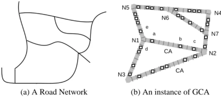
We model a road network with a graph of cellular au-tomata (GCA), where the nodes of the graph represent road intersections and the edges represent road segments with
N1 N2 N3 N4 a b N5 N6 N7 c d e CA CA
(a) A Road Network (b) An instance of GCA
Figure 1: An example of a road network and its GCA model
no intersections. Different from the general graph model, each edge in the GCA consists of a cellular automaton (CA), which is represented, in a discrete mode, as a finite sequence of cells. Each cell corresponds in practice to some road seg-ment of about 7.5 m.
Figure 1 shows an example of a road network and its GCA model. Each node has a label which represents an intersection of the road network. The wide lines represent edges and each edge treated as one CA connects many cells. The CA model was used in this context by [12]. We first recall the definition of cellular automaton.
Definition 1 A cellular automaton consists of a finite ori-ented sequence of cells. In a configuration, each cell is either empty or contains a symbol. During a transition, symbols can move forward to subsequent cells, symbols can leave the CA and new symbols can enter the CA.
An example of cellular automaton corresponding to edge
(N1, N2) in Figure 1(b) with a transition between two
con-figurations is given in Figure 2. We now formally define a graph of cellular automata.
Definition 2 The structure of a GCA is a directed weighted graph G = (V, E, l) where V is a set of vertices (i.e.,
nodes), E is a set of edges and l : E → N is a function
which associates to each edge the number of cells of the corresponding cellular automaton.
We assume a countably infinite alphabet Ω : {α, β, γ, · · ·}, denoting moving objects’ names. Let C be
the set of cells of a GCA.
A configuration or an instance of a GCA, is a mapping from the cells of the GCA to constants inΩ together with
a given velocity. Intuitively, the velocity is the number of cells an object can traverse during a time unit.
Definition 3 An instance I of a GCA is defined by two func-tions:
µ: C → ΩS{ε} (1-1 mapping) v: Ω →N.
A moving object is represented as a symbol attached to the cell in the GCA and it can move several cells ahead at each time unit. Figure 1(b) is an instance of the GCA corre-sponding to the road network of Figure 1(a). In Figure 1(b), moving objects are denoted by squares. A moving object lies on exactly one cell of the edge and its location can be obtained by computing the number of cells relative to the start node. For instance, object α lies on the edge(N1, N2)
and there are two cells away from N1along the edge.
There-fore, its position can be expressed by(N1, N2,2).
The motion of an object is represented as some (time, location) information. Representing such information of a moving object as a trajectory is a typical approach [20]. In the GCA model, the trajectory of a moving object can be divided two types: the in-edge trajectory for the object’s movement in one edge (CA) and the global trajectory for the object that may move cross several edges (CAs) dur-ing its movement. The in-edge trajectory of an object is a polyline in two-dimensional space (one-dimensional rela-tive distance, plus time), which can be defined as follows: Definition 4 The in-edge trajectory of a moving object in a CA of length L is a piece-wise function f : T → N,
represented as a sequence of points (t1, l1), (t2, l2), . . . , (tn, ln)(t1< t2< . . . < tn, l1< l2< . . . < ln≤ L).
When an object moves across multiple edges, its global trajectory is defined as functions mapping the time to the edge and relative distance.
Definition 5 The global trajectory of a moving ob-ject in different CAs is a piece-wise function f : T → (E,N), represented as a sequence of points (t1, e1, l1), . . . , (ti, ej, lk), . . . , (tz, em, ln)(t1 < t2 < . . . < tz).
In the sequel, we will be interested by deterministic paths in the GCA i.e., path with source nodes of out degree 1. The successive CAs in a deterministic path can be then seen as a unique CA.
Let i be an object moving along an edge. Let v(i) be
its velocity, x(i) its position, gap(i) the number of empty
cells ahead (forward gap), and Pd(i) a randomized
slow-down rate which specifies the probability it slows slow-down. We assume that Vmaxis the maximum velocity of moving
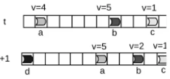
ob-jects. The position and velocity of each object might change at each transition as shown definition 6 adapted from [12]. Definition 6 At each transition of the GCA, each object changes velocity and position in a CA of length L according to the rules below:
1. if v(i) < Vmaxand v(i) < gap(i) then v(i) ← v(i)+1
t t+1 a b c a b c v=4 v=5 v=1 v=5 v=2 v=1 d
Figure 2: Transition of the GCA
3. if v(i) > 0 and rand() < Pd(i) then v(i) ← v(i) − 1
4. if(x(i) + v(i)) ≤ L then x(i) ← x(i) + v(i)
The first rule represents linear acceleration until the ob-ject reaches the maximum speed Vmax. The second rule
ensures that if there is another object in front of the current object, it will slow down in order to avoid collision. In the third rule, the Pd(i) models erratic movement behavior.
Fi-nally, the new position of object i is given by the fourth rule as the sum of the previous position with the new velocity if it is in the CA. Note that it is easy to extend the definition of transition to deterministic paths. Because of determinis-tic path, the objects move to a new position in a subsequent CA. Figure 2 shows the simulated movement of objects on a cellular automaton of the GCA in two consecutive times-tamps. We can see that at time t, the speed of the object a is smaller than the gap (i.e. the number of cells between the object a and b). On the other hand, the object b will reduce its speed to the size of the gap. According to the fourth rule, the objects move to the corresponding positions based on their speeds at time t+ 1.
However, objects in real traffic have different desired speed. With the transitions of the GCA of one lane CA mentioned above, it can be found that slow objects being followed by faster ones, and the average speed reduced to the free-flow speed of the slowest object [11]. In view of this, we extend the one lane GCA to two lane GCA in which a CA consists of two parallel single lane. Therefore, each cell in two lane GCA is composed of two parallel single lane and each lane may contain one symbol namely a mov-ing object. The function µ in a GCA instance I will change to the 1-2 mapping accordingly.
For the transition of GCA with one lane, we extend it to the two lane by attaching an additional rule that models the changing of lanes of the object. Suppose the objects move only sideways, the transition of GCA happens on both lanes according to the previous four rules and then the exchange of objects between two lanes is checked according to the additional conditions for changing lane as follows:
5. object i changes lane with probability Pcif
gap(i) < p, gapo(i) > p1, and gapo,b(i) > po,b
where gap(i) is the number of empty cells ahead in
the same lane, gapo(i) is the forward gap on the other
p=3, po=3, po,b=5
a b c d
e
Figure 3: An example of changing lane in transition of the two
lane GCA
lane, gapo,b(i) is the backward gap on the other lane, p, poand po,bare the parameters which decide how far
the object looks ahead on the current lane, ahead on the other lane, and back on the other lane, respectively. In fact, the changing lane rule is based on the following observation: the car looks ahead if some car is in its way; the car looks on the other lane if it is any better there; the car looks back on the other lane if it would get in other cars way. Generally, in the above rule, both p and poare
essen-tially proportional to the velocity, whereas looking back de-pends mostly on the expected velocity of other objects, not on one’s own. An example of invoking the rule of changing lane with p= v + 1, po= p, po,b= vmax, Pc= 1 is given
in Figure 3. The object b with p = 3, po = 3, po,b = 5
changes to the other lane in the GCA due to satisfying the fifth rule mentioned above.
4
Trajectory Prediction
In the management of moving objects, the trajectory pre-diction method is usually used to improve the performance of the location update strategy and to support the predictive index and queries. In this part, we first review some linear prediction methods and analyze their problem in handling moving objects in constrained networks, and finally present our simulation-based prediction method.
4.1 The Linear Prediction (LP)
Most current index and query processing approaches use the linear prediction method for its simplicity and capabil-ity of approximating any curve of free movement by piece-wise linear segments. Suppose the trajectory function for an object between time t0and t1is
~
Xt= ~Xt0+ ~V(t − t0) (t0≤ t ≤ t1)
where ~Xt0denotes the position of the object at time t0and
~
V denotes the velocity of the object, which is assumed to
remain fixed between t0to t1.
General LP The general linear prediction method uses the object’s current position ~Xt0and current velocity ~V to
pre-dict its position in the near future. When the prepre-diction is deemed inaccurate, that is, its deviation from the actual po-sition is beyond a predefined threshold, we revise our pre-diction by resetting ~Xt0and ~V . In situations where object’s
d t real trajectory predicted function t d real trajectory simulated trajectory linear regression function
(a) General Linear Prediction (b) Simulation-based Prediction
Figure 4: Linear Prediction VS. Simulation-based Prediction
make future prediction with high precision. However, when objects move with changing velocity, their trajectory func-tions have to be revised frequently.
Road Segment Based LP If objects move in a constrained environment such as a transportation network, we can use the road segments of the network to help model the object’s movement. In other words, we assume objects move at con-stant speed along a road segment, that is, their trajectory functions will not change until they move out of a road seg-ment. When an object enters a new road segment, we re-set the velocity ~V in its trajectory function. The frequency
of revising the trajectory function depends on the average length of the road segments.
Route Based LP If objects have regular and known routes in the transportation network (e.g., one takes the same route from home to work), we can use the routes instead of the road segments to reduce the number of updates needed to maintain the objects’ position. If the route is predicted in-correctly, we simply make an additional update.
However, any real traffic system has a stochastic, dy-namic and fuzzy nature. The accuracy of linear predic-tion methods menpredic-tioned above is inadequate because linear methods can hardly reflect the movement of objects con-strained by road networks. For example, in urban road net-works, because of traffic conditions, a vehicle may travel at a constant speed, decelerate to stop, wait, accelerate and travel again at a constant speed. Vehicles may often repeat the above movement in modern urban road networks.
We use Figure 4 to demonstrate the inadequacy of the linear prediction method for real road networks. Figure 4(a) shows the predicted (linear) trajectory and the actual trajec-tory of an object. We can see that each time the change of the object’s velocity is above a certain threshold, an update is triggered and the trajectory is revised by a new velocity vector. The frequent changes of the object’s velocity will incur repeated update and prediction.
4.2 The Simulation-based Prediction (SP)
Considering the simulation feature of the GCA model, we use GCAs not only to model road networks, but also to simulate future trajectories of moving objects by the tran-sitions of GCAs, where objects’ movement follows traffic rules. Based on the GCA, a Simulation-based Prediction (SP) method to anticipate future trajectories of moving ob-jects is proposed. The SP method treats the object’s sim-ulated results as its predicted positions to obtain its future in-edge trajectory. To refine the accuracy, based on differ-ent assumptions on the traffic conditions we simulate two future trajectories in discrete points for each object on its edge. Then, by linear regression and translating, the tra-jectory bounds that contain all possible future positions of a moving object on that edge can be obtained. When the object moves to another edge in the GCA or the predicted position exceeds its actual position above the predefined ac-curacy, another simulation and regression will be executed to predict new future trajectory bounds. The process of the simulation-based prediction can be seen in Figure 5.
Most existing work uses the CA model for traffic flow simulation in which the parameter Pd(i) is treated as a
ran-dom variable to reflect the stochastic, dynamic nature of traffic system. However, we extend this model for pre-dicting the future trajectories of objects by setting Pd(i) to
values that model different traffic conditions. For exam-ple, laminar traffic can be simulated with Pd(i) set to 0 or
a small value, and the congestion can be simulated with a larger Pd(i). By giving Pd(i) two values, we can derive two
future trajectories, which describe, respectively, the fastest and slowest movements of objects as showed in Figure 5(a). In other words, the object’s future locations are most prob-ably bounded by these two trajectories. The value of Pd(i)
can be obtained by the experiences or by sampling from the given dataset. Our experiments show one of methods to choose the value of Pd(i). It is proved that 0 and 0.1 are
realistic values of Pd(i) in our cases.
For getting the future trajectory function of an object from the simulated discrete points, we need to regress the discrete positions. We find that in most cases the linear regression (as shown in Figure 4b) fits the prediction well and at low cost. The OLSE (Ordinary Least Square Estima-tion) method, for example, can be calculated efficiently with low data storage cost. Let the discrete simulated points be
(t1, d1), . . . , (ti, di), . . . , (tn, dn), where di(i∈ [1, n])
de-notes the relative distance in an edge and the average value be t and d. After regression, the trajectory function of the moving object is:
D(t) = ˆβ0+ ˆβ1· t
where ˆβoand ˆβ1are given by:
ˆ
t d slowest movement fastest movement simulated trajectory regress function t d upper bound lower bound
(a) Simulated trajectories (b) Two predicted bounds
Figure 5: Two Predicted Bounds of Future Trajectories
ˆ β1 = Pn i=1tidi− nt · d Pn i=1t 2 i − n(t) 2
In Figure 5(a), the dashed curves show two future tra-jectories, which are the slowest and the fastest movements simulated by using different Pd. Applying the OLSE
algo-rithm to the two trajectories generates two linear functions, which are shown in solid lines.
fastTrj: D(t) = αf· t + γf slowTrj: D(t) = αs· t + γs
Finally, in order to find the bounds of the area that contains all estimated future positions, we translate the two regression lines, until all estimated future positions fall within. More specifically, we translate the upper line (fastest movement) upwards until it touches the point with the max residual (denoting ǫ1 the distance translated
up-ward), and similarly, we translate the lower line (slowest movement) downwards (denoting ǫ2the distance translated
downward). This minimizes the loss of information and er-rors brought by the OLSE algorithm.
We now define the two bound lines as the upper bound and lower bound of objects’ future trajectory.
Definition 7 The upper bound of an object trajectory
upperBound is the upper bound line of its fastest future
trajectory, and the lower bound lowerBound is the lower bound line of its slowest future trajectory. They are linear functions of the following form:
upperBound: D(t) = αf· t + λf lowerBound: D(t) = αs· t + λs
where λf= γf+ ǫ1, λs= γs− ǫ2.
The two bound lines are shown in Figure 5(b). we can treat the two predicted lines as the bounds of the possi-ble future positions of one object. The predicted trajec-tory bounds can be used in the predictive index structure and query processing in road network to reduce the index updates and filter unnecessary query results to improve the
t d slowest movement fastest movement simulated trajectory regress function t d slowest movement fastest movement a L1 L2 L3 predicted function simulated trajectory
(a) Simulated trajectories (b) Single predicted function
Figure 6: Singe Predicted Future Trajectory
performance of predictive query. For example, given a pre-dictive range query with the specified region R during time interval[t1, t2] in the future, we can filter the objects in the
result during the pre-process phase if the area between their upper and lower trajectory bounds can not intersect the R during[t1, t2].
However, for other applications such as the tracking of moving objects, a single predicted function is needed to ob-tain the specific future positions of the object. For example, to lower update frequency from moving objects to server database, a general principle for location update policies is as follows: the moving objects equipped by GPS receiver do not report their locations to the server unless their actual positions exceed the predicted positions to a certain thresh-old. Their predicted positions need to be computed by a single predicted function. In this case, we can also adapt the SP method to obtain a compact and simple linear pre-diction function. The process can be seen in Figure 6. After regressing the two simulated future trajectories to two lin-ear function denoting L1and L2 , we compute the middle
straight line L3, the bisector of the angle a between L1and L2as the final predicted function L(t).
Although the predicted function obtained by the SP method is a simple linear function, it is different from the linear prediction in that the SP method not only consid-ers the speed and direction of each moving object, but also takes correlation of objects as well as the stochastic behav-ior of the traffic into account. The experimental results also show it is a more accurate and effective prediction approach. As the prediction of in-edge trajectory only use the GCA to simulate the movement of objects in an edge, we have to consider the cases when objects move across the nodes in order to make the global trajectory prediction. If the out degree of a node in the GCA is one, the behavior of the object in the adjacent edge is the same. However, if the out degree of the node is bigger than one, we can not trace the objects cross the different edges. In this case, we could use the probability of objects changing the edges accord-ing to the historical data. In this paper, we only predict the in-edge trajectory of the object moving in one edge of the
GCA. When the object moves to another edge or its predic-tion accuracy of the future posipredic-tions cannot arrive the given accuracy requirement, we issue another prediction based on the current traffic conditions.
5
Experimental Evaluation
We evaluate the simulation-based prediction method by comparing it with the general linear prediction method. Us-ing two datasets (generated by the CA simulator and by the Brinkhoff’s Network-based Generator [3]), we measure their prediction accuracy when applied to predict the near anticipated future positions in the real map network. We also study the effect of the choice of different values of the parameter Pdon the simulation-base prediction.
Datasets
We use two datasets for our experiments. The first is generated by the CA simulator, and the second by the Brinkhoff’s Network-based Generator [3]. We use the CA traffic simulator to generate a given number of objects in a uniform network of size10000 × 10000 consisting of 500
edges. Each object has its route and is initially placed at a random position on its route. The initial velocities of the objects follow a uniform random distribution in the range
[0, 30]. The location and velocity of every object is updated
at each time-stamp.
The Brinkhoff’s Network-based Generator has been used as a popular benchmark in the related work of the MOD. The generator takes a map of a real road network as input (our experiment is based on the map of Oldenburg includ-ing 7035 edges). The positions of the objects are given in two dimensional X-Y coordinates. We transform them to the form of(edgeid, pos), where edgeid denotes the edge
identifier and pos denotes relative position on the edge. The generator places a given number of objects at random posi-tions on the road network, and updates their locaposi-tions at each time-stamp. Each object has its own destination, and it moves toward its destination along a given route. Prediction Accuracy and Cost
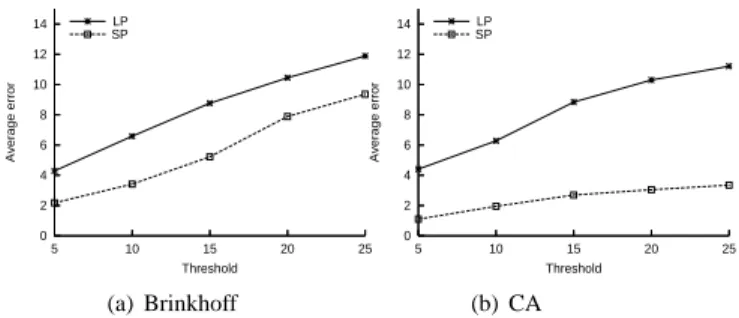
We compare the precision of the SP method with the LP method. We measure the prediction accuracy by “average error” but with different threshold. The threshold represents the maximum deviation between the predicted locations of a moving object and its real locations allowed in the predic-tion. That means when the deviation exceeds the threshold, we make another prediction. From Figure 8, we observe that average error will increase when threshold increases. This is because the larger the threshold is, the larger the de-viation becomes, which leads to the more errors. This is tenable in both the LP and SP method. However, the SP method predicts more accurately than the LP method with any threshold. 0 2 4 6 8 10 12 14 25 20 15 10 5 Average error Threshold LP SP (a) Brinkhoff 0 2 4 6 8 10 12 14 25 20 15 10 5 Average error Threshold LP SP (b) CA
Figure 7: Prediction Accuracy with Different Threshold
9.7 9.8 9.9 10 10.1 10.2 10.3 0.5 0.4 0.3 0.2 0.1 0 Average error Pd (a) Average Error
0 0.1 0.2 0.3 0.4 0.5 0.5 0.4 0.3 0.2 0.1 0 Overflow rate Pd (b) Overflow Rate
Figure 8: Prediction Accuracy with Different Pd
The time complexity of the simulation-based predic-tion depends on many factors. We compute the average CPU time when simulating and predicting the movement of one object along the edge with length 1000 in different dataset sizes. The results show that the average cost of one simulation-based prediction is about 0.25ms. This is quite acceptable.
The Slowdown Rate Pd
The CA simulation has an important effect on the accu-racy of the simulation-based prediction. We study the effect of the choice of different Pd, which determines the two
pre-dicted trajectories corresponding to the fastest and slowest movement. We test on the Brinkhoff dataset with different data size and use Pdfrom 0 to 0.5 and measure the average
prediction accuracy by “average error” and “overflow rate”. The average error is the average absolute error between the predicted and actual positions, and the overflow rate rep-resents the probability of predicted positions exceeding the actual positions. The purpose of this metric is to find the closest two trajectories binding the actual one as future tra-jectories. In this way, we can choose the Pdboth with lower
average error and overflow rate. Figure 8 shows the predic-tion accuracy of the SP method with different slowdown rates. We can see that when Pd is set to 0 and 0.1, both
the average error and overflow rate are lower than others. Therefore, we use the value 0 and 0.1 as slowdown rates for the fastest movement bound and the slowest movement bound to obtain better prediction results.
6
Conclusion
Managing moving objects in a constrained network is a challenging task as well as of great practical importance in mobile location-aware applications. It is necessary to rep-resent and predict the future trajectories of moving objects more accurate. In this paper, we first combine road network representation and the movement model of objects in a traf-fic network to introduce a new model - GCA for network-constrained moving objects. And then we propose a predic-tion method, based on the GCA, which predicts with a great accuracy the future trajectories of moving objects. The ac-curacy results from the fact that the GCA model exploits the constraints of the network and models the stochastic as-pect of urban traffic. Our experimental results performed on two datasets show that the prediction accuracy of our simulation-based prediction is higher than the linear predic-tion used in the predictive indexing and query processing.
Acknowledgment
This research was partially supported by the grants from the Natural Science Foundation of China under grant num-ber 60573091, 60273018; the Key Project of Ministry of Education of China under Grant No.03044; Program for New Century Excellent Talents in University (NCET); Pro-gram for Creative PhD Thesis in University and performed in the framework of a joint project with INRIA. The au-thors would like to thank Zhen Xiao, Benzhao Li from In-formation school, Renmin University of China for the assis-tance of experimental evaluation and Karine Zeitouni from PRISM, Versailles Saint-Quentin University in France for many helpful advice and assistance.
References
[1] C. Aggarwal, D. Agrawal. On Nearest Neighbor Index-ing of Nonlinear Trajectories. In PODS, 2003, 252-259. [2] V. T. Almeida, R. H. G¨uting. Indexing the Trajectories of Moving Objects in Networks (Extended Abstract). In SSDBM, 2004, 115-118.
[3] T. Brinkhof. A framework for generating network-based moving objects. In GeoInformatica, 6(2), 2002, 153-180.
[4] H. D. Chon, D. Agrawal, A. E. Abbadi. Using Space-Time Grid for Efficient Management of Moving Ob-jects. In MobiDE 2001, 59-65.
[5] A. Civilis, C. S. Jensen, S. Pakalnis. Techniques for Ef-ficient Road-Network-Based Tracking of Moving Ob-jects. In IEEE Trans. Knowl. Data Eng. 17(5): 698-712 (2005).
[6] Y. Cai, N. Raymond. Indexing spatiotemporal trajecto-ries with chebyshev polynomials. In SIGMOD, 2004, 599-610.
[7] Z. Ding, R. H. G¨uting. Managing Moving Objects on Dynamic Transportation Networks. In SSDBM, 2004, 287-296.
[8] E. Frentzos. Indexing objects moving on Fixed net-works. In SSTD, 2003, 289-305.
[9] R. H. G¨uting, M. H. B¨ohlen , M. Erwig, C. S. Jensen, N. A. Lorentzos, M. Schneider, M. Vazirgiannis. A Foun-dation for Representing and Querying Moving Objects. In TODS 25(1), 1-42(2000).
[10] M. Kolahdouzan, C. Shahabi. Voronoi-Based K Near-est Neighbor Search for Spatial Network Databases. In VLDB 2004, 840-851.
[11] T. Nagatani. Bunching of cars in asymmetric exclu-sion models for freeway traffic, Phys. Rev. E 51(N2), 922 (1995).
[12] K. Nagel, M. Schreckenberg. A cellular automaton model for freeway traffic. Journal Physique I 2, 1992, 2221-2229.
[13] D. Papadias, J. Zhang, N. Mamoulis, Y. Tao. Query Processing in Spatial Network Databases. In VLDB, 2003, 790-801.
[14] L. Speicys, C. S. Jensen, A. Kligys. Computational Data Modeling for network-Constrained Moving Ob-jects. In ACM-GIS, 2003, 118-125.
[15] C. Shababi, M.R. Kolahdouzan, M. Sharifzadeh. A Road Network Embedding Technique for K-Nearest Neighbor Search in Moving Objects Databases. In GeoInformatica 7(3), 2003, 255-273.
[16] P. Sistla, O. Wolfson, S. Chamberlain, S. Dao. Model-ing and QueryModel-ing MovModel-ing Objects. In ICDE 1997, 422-432.
[17] J. Su, H. Xu, O. Ibarra. Moving Objects: Logical Re-lationships and Queries. In SSTD 2001, 3-19.
[18] Y. Tao, C. Faloutsos, D. Papadias, B. Liu. Prediction and Indexing of Moving Objects with Unknown Motion Patterns. In SIGMOD, 2004, 611-622.
[19] Y. Tao, D. Papadias, J. Zhai, Q. Li. Venn Sampling: A Novel Prediction Technique for Moving Objects. In ICDE, 2005, 680-691.
[20] M. Vazirgiannis, O. Wolfson. A Spatiotemporal Model and Language for Moving Objects on Road Net-works. In SSTD, 2001, 20-35.
[21] O. Wolfson, B. Xu, S. Chamberlain, L. Jiang. Mov-ing Object Databases: Issues and Solutions. In SSDBM 1998, 111-122.