HAL Id: hal-03125706
https://hal.inrae.fr/hal-03125706
Submitted on 9 Jun 2021HAL is a multi-disciplinary open access archive for the deposit and dissemination of sci-entific research documents, whether they are pub-lished or not. The documents may come from teaching and research institutions in France or abroad, or from public or private research centers.
L’archive ouverte pluridisciplinaire HAL, est destinée au dépôt et à la diffusion de documents scientifiques de niveau recherche, publiés ou non, émanant des établissements d’enseignement et de recherche français ou étrangers, des laboratoires publics ou privés.
Towards a better understanding of grass bed dynamics
using remote sensing at high spatial and temporal
resolutions
Menu Marion, Papuga Guillaume, Andrieu Frédéric, Debarros Guilhem,
Fortuny Xavier, Alleaume Samuel, Pitard Estelle
To cite this version:
Menu Marion, Papuga Guillaume, Andrieu Frédéric, Debarros Guilhem, Fortuny Xavier, et al.. Towards a better understanding of grass bed dynamics using remote sensing at high spatial and temporal resolutions. Estuarine, Coastal and Shelf Science, Elsevier, 2021, 251, pp.107229. �10.1016/j.ecss.2021.107229�. �hal-03125706�
Title: Towards a better understanding of grass bed dynamics using remote sensing at high spatial and temporal resolutions
Authors: Menu Marion12, Papuga Guillaume345, Andrieu Frédéric4, Debarros Guilhem4,
Fortuny Xavier6, Alleaume Samuel1, Pitard Estelle27
1. UMR TETIS, INRAE, AgroParisTech, CIRAD, CNRS, Université de Montpellier, 500 rue Jean-François Breton, 34093 Montpellier Cedex 5, France
2. UMR 5221 Laboratoire Charles Coulomb, CNRS, Université de Montpellier, Batiment 13, Campus Triolet, Université de Montpellier, CC069, 34095 Montpellier, France
3 . UMR 5175 Centre d’Écologie Fonctionnelle et Évolutive, CNRS, 1919 route de Mende, 34293 Montpellier cedex 5, France.
4. Conservatoire Botanique National Méditerranéen de Porquerolles, antenne Languedoc-Roussillon, parc scientifique Agropolis-B7, 2214 boulevard de la Lironde, 34980 Montferrier sur Lez, France
5. UMR AMAP, Université de Montpellier, IRD, CNRS, CIRAD, INRAe, Montpellier, France.
6. ADENA, Réserve Naturelle Nationale du Bagnas, Agde, France
7. Department of Environmental Science, Policy and Management, University of California, Berkeley, CA 94720, USA Orcid: – Papuga G.: https://orcid.org/0000-0002-7803-2219 – Alleaume S.: https://orcid.org/0000-0002-9200-8338 1 2 3 4 5 6 7 8 9 10 11 12 13 14 15 16 17 18 19 20 21 22 23 24
Abstract
Wetlands conservation and resilience capacities are key issues in many places over the globe. Understanding these issues will benefit from a precise knowledge of seagrass species occupancy and coverage over time and over space. Such information can be obtained from remote sensing images and their classification thanks to a vegetation index, to be used in a complementary manner to field work inventories. Sentinel-2 data, which are available with a frequent revisit time (<5 days) and a high spatial resolution (10m pixel size) can be used to map grassbeds at the surface or slightly below the surface of permanent lagoons, hence enabling the characterization of its seasonal dynamics, which was not possible with previous remote-sensing tools. We have proved the feasibility of such a method in the natural reserve of the Bagnas (Herault, France) where Stuckenia pectinata coverage can be tracked over a full year thanks to Sentinel-2 images and field work. Inter-annual dynamics (seasonal growth and senescence) can be mapped over time with 10m resolution and will be extended to pluriannual studies thanks to the long-term objective of the Sentinel-2 mission. This opens the way to a concerted management of natural reserves based on data analysis and field knowledge, a better understanding of seagrass coverage with fluctuating environmental conditions, and predictive mechanistic and/or stochastic models of future qualitative trends.
Keywords: Remote sensing – temporal survey – mesohaline lagoon – National Natural Reserve of the Bagnas (France) – pondweed grass beds – Sentinel-2 satellites – Stuckenia
pectinata – ecosystem management – ecological indicator – wetlands conservation
25 26 27 28 29 30 31 32 33 34 35 36 37 38 39 40 41 42 43 44 45 46 47 48
Introduction
Wetland conservation has become a cornerstone of conservation biology, as these habitats represent high biodiversity areas, and critical human resources in terms of water (Pereira et al., 2009), food supply, and eventually recreational areas (Newton et al., 2018). Consequently, they are under global pressure due to the intensive use of water and change of soil occupation, which both threaten wildlife and disrupts ecosystem services (Gaertner-Mazouni and De Wit, 2012). Coastal lagoons are transition waters between continental and marine domains, filled with brackish water in which salinity may vary over time. They exemplify wetland conservation issues since they are highly diversified habitats of significant conservation value (Pérez-Ruzafa et al., 2011). At the same time, they have to face ever-increasing human impacts due to the development and urbanization of coastal areas (Pojana et al., 2007) and land use throughout the catchment area (Cañedo-Argüelles et al., 2012; Shili et al., 2007). Lagoons also represent essential habitats for a variety of taxa: they are a privileged stopover for migrating birds (Holm and Clausen, 2006); they constitute nurseries for sea fishes (Yamamuro, 2012); they host many plants (both angiosperms and algae) specific to these habitats (Hartog, 1981). Variation in salt concentration is a significant determinant of ecosystem functioning and profoundly impacts biodiversity. Thus, water input shapes the biodiversity of such ecosystems and can trigger drastic changes over short periods (Obrador and Pretus, 2010; Shili et al., 2007; Antunes et al., 2012).
International awareness of those conservation issues has led to the introduction of protection treaties, such as the Ramsar treaty (Gardner and Davidson, 2011). At the European level, two directives have been set up to protect those habitats. First, the Water Framework Directive (WFD) aims at preserving European waters in a good quality state (Chave, 2001). This convention covers all water bodies from rivers to lakes larger than 0,5 km2, including
coastal lagoons. In parallel, the Habitats Directive (HD) has defined a list of protected habitats and aims at maintaining their good conservation status to preserve wildlife over long time periods. Lagoons represent one particular habitat, named "habitat 1150 – Coastal lagoon". Additionally, different national initiatives have added layers to the protection of such areas. In France, the National Natural Reserve network includes several lagoons, which ensures land protection and allows the implementation of management plans tackling biodiversity issues (Therville et al., 2012).
Within lagoons, grass beds represent a key compartment of the ecosystem. They are primary producers that provide food and produce oxygen, which is essential to many organisms (Camacho et al., 2012; Scheffer, 1997). They constitute shelters for a whole range of animals, including fishes and invertebrates (Benedetti-Cecchi et al., 2001; Lloret and Marín, 2009). The analysis of their composition and dynamics inform on the ecosystem functioning, regarding both abiotic compartment of the ecosystem (e.g. water and soil characteristics) and biotic interactions (Camacho et al., 2012). Water quality strongly influences grass beds, as salt and trophic levels influence plant development and survival (Obrador and Pretus, 2010). Eutrophication is a critical issue as it might lead to a dystrophic crisis when oxygen decreases to the point where wildlife dies because of anoxic conditions (Duarte et al., 2002). Such changes in abiotic conditions can lead to sharp temporal transitions in plant community composition and structure (i.e. grassbed extent) that in return deeply modify the functioning of the whole waterbed (Obrador and Pretus 2010, Antunes et al. 2012, Perez-Ruzufa et al, 2011), including nutrient cycling (Duarte et al. 2002). Therefore, 49 50 51 52 53 54 55 56 57 58 59 60 61 62 63 64 65 66 67 68 69 70 71 72 73 74 75 76 77 78 79 80 81 82 83 84 85 86 87 88 89 90 91 92 93
understanding grass bed dynamics is an efficient surrogate to ecosystem functioning and is a prime indicator to manage such a system.
Legal protection usually assigns biodiversity management as the primary mission of protected areas, intending to ensure the long-term persistence of biodiversity on the territory. Implementing efficient conservation strategies requires accurate tools to detect the effect of changes in the system, and grass beds represent key indicators to understand ecosystem dynamics. However, quantifying grass beds dynamics is a complex task, due to the inherent difficulty to access such vegetation (Silva et al. 2008), and assess such highly varying intra-annual dynamics through the required frequent temporal revisits (Shili et al., 2007; Antunes et al., 2012). Additionally, the protection status of some lagoons prohibits the use of intrusive and destructive sampling methods, and restrain access to such areas to limit disturbance of animals. Collecting and maintaining up-to-date and regular information on grassbed distribution is a major challenge (Antunes et al. 2012).
In this context, the use of remote sensing is a powerful way to characterize the dynamics of such vegetation without impacting this environment. Lagoons were among the first to be studied when remote sensing methods emerged 20 years ago (see the review on pioneering works by Lehmann and Lachavanne, 1997). At that time, those new methods had to face sharp criticisms because they were expensive (Silva et al., 2008) and produced inaccurate results (Cazals et al., 2016; Vis et al., 2003). These approaches have seen their performances rapidly improving over the last ten years and are now increasingly used in ecological researches (Veetil et al, 2020). Yet, such methods have failed so far to enter the current monitoring scheme of most natural reserves due to their high cost and complexity of treatment. Moreover, studies either focused on high resolution/low frequency (i.e. once a year) data (e.g. Khanna 2011, which uses a hyperspectral detector able to distinguish between different species of seagrass), or low resolution/high frequency data, typically based on Landsat images (Lyons et al, 2013)
Today, the emergence of new satellites that produce repeated images free of cost boosts the development of such technology, and allow ecologists to get insights into seasonnal dynamics of grass beds, a dimension that was hardly accessible before (Traganos et al 2018, Kohlus et al, 2020). In particular, as part of the European Union Copernicus program, the two Sentinel-2 satellites produce images every 5 days, at a high spatial resolution of 10 m. Each satellite carries a single multispectral instrument with 13 spectral channels within visible, near-infrared, and shortwave infrared spectra, which are particularly adapted to detect vegetation. This massive flow of earth observation data provides a rich and detailed description of ecosystems, allowing their condition and evolution to be monitored. It is thus possible to analyze intra- and inter-annual changes in ecosystems at a fine-scale or monitor the evolution of the phenology of various ecosystems. The seasonal dynamics of intertidal grassbeds was investigated in Zoffoli et al, 2020, at low tide.
Through this article, we model the growth and persistence dynamics of lagoon grass beds using remote sensing approaches based on images from the Sentinel-2 satellite, and we choose the Bagnas Natural Reserve located in the south of France as a model ecosystem. We model the intra-annual (i.e. seasonnal) dynamics of such a system during the year 2017 thanks to high quality repeated images produced every two weeks. Firstly, we differentiate aquatic vegetation (which can be either submerged or lying at the water surface) from peripheric reedbeds belts to precisely delimit the open-water lagoon extent. Secondly, we develop two approaches to delineate grass beds based on simple spectral indices thresholds and Spectral 94 95 96 97 98 99 100 101 102 103 104 105 106 107 108 109 110 111 112 113 114 115 116 117 118 119 120 121 122 123 124 125 126 127 128 129 130 131 132 133 134 135 136 137 138 139
Linear Unmixing approaches. Finally, we compare these two approaches and validate them with a field map realized in summer 2017 to assess the accuracy of our methods. We discuss how such a methodology can be extended to other lagoon ecosystems worldwide.
Materials & methods
1. Study site
Coastal lagoons are well represented in the south of France, especially west of the Rhône delta (i.e. the Camargue region) where the coast (i.e. Gulf of Lion) is formed by sedimentary deposits. Located in the city of Agde (Hérault, France), the Bagnas (Figure 1) is a National Natural Reserve since 1983 and Natura 2000 site since 2004. It is composed of several lagoons of various sizes whose functioning includes temporary and permanent water bodies. The central lagoon (named "Grand Etang du Bagnas") is a coastal lagoon of approximately 190 ha. The catchment area measures 805 ha, and is mostly occupied by agricultural activities (including vineyard) and urbanization.
Most of the water supply (66%) corresponds to freshwater coming from the Hérault stream through the Canal du Midi (Agbanrin, 2018). The rest is brought by rainwater (34%). The lagoon is hydraulically managed to preserve qualitatively biodiversity issues, especially for water birds. This management consists mainly of controlling inflows and outflows to maintain water levels compatible with the ecological requirements of species. As a result, water levels are maintained at about 85 cm between December and March to support wintering stationing of waterbirds species. From the beginning of spring, the water levels are lowered until reaching 40 cm in August to allow the nesting of specific target species and also to make the lagoon attractive for migratory birds next fall (however, there are fluctuations and discrepancies between target water levels and measured water levels, see Appendix 1). Thus, its salinity is comprised between 5 and 20g/L, and fluctuates throughout the year depending on water inputs, making it a mesohaline lagoon (Grillas et al., 2018).
The lagoon is surrounded by reed beds and is extensively covered by a grass bed almost exclusively composed of pondweed (Stuckenia pectinata (L.) Börner 1912). The grass bed stretches to its maximum extent during the summer (August-September) and disappears during winter. When plants reach their maximum development, their leaves attain the surface and entirely cover parts of the water body. It constitutes an essential resource for migratory birds, especially ducks that feed on leaves and/or seeds (Arzel et al., 2006). Two other species can be occasionally found: Ruppia cirrhosa (Petagna) Grande, 1918 is an angiosperm sparsely distributed throughout the lagoon, most of the time represented by few individuals;
Lamprothamnium papulosum (K.Wallroth) J.Groves, 1916 is a Characeae that occasionally
appears below grass beds, and never reaches the surface. 140 141 142 143 144 145 146 147 148 149 150 151 152 153 154 155 156 157 158 159 160 161 162 163 164 165 166 167 168 169 170 171 172 173 174 175 176
Figure 1: Map of the Bagnas Reserve region of interest. The full reserve limit is in red, while the Grand Bagnas where our study focuses is limited by the blue line.
2. Satellite images
To detect grass beds, we used Sentinel-2 multispectral images with 10m resolution bands: blue (B2), green (B3), red(B4), and near-infrared NIR (B8). These images are produced by two satellites (Sentinel 2A and 2B) launched by the European Spatial Agency (ESA) thanks to the Copernicus program of the European Union. They allow accessing images of the same area every 5 days. ESA produces and distributes Level 1C ortho-rectified data expressed in reflectance at the top of the atmosphere. Theia platform (theia.cnes.fr) produces and distributes level 2A data, corrected for atmospheric effects thanks to the MAJA software (Hagolle et al., 2017). This processor uses multi-temporal information to detect clouds and clouds' shadows to estimate the optical properties of the atmosphere. Thanks to the high temporal frequency of the Sentinel-2 instrument, we could work with a temporal series of 32 high-quality cloud-free images taken between January 13th 2017, and April 13th 2018.
Early 2018 images were conserved to assess the date of minimal expansion of the grassbed, as mediterranean winter does not coincide strictly with calendar year.
3.Field data
During summer 2017, we launched a field campaign to map the distribution of the grass bed. We set up 103 sampling points following a systematic grid of 200m, doubled 178 179 180 181 182 183 184 185 186 187 188 189 190 191 192 193 194 195 196 197 198 199
within the first 100m from the pond border to improve the detection of vegetation variability (personal communication P. Grillas, 2016). Each point was sampled by boat at the end of July 2017; first, we recorded the frequency of each species of the community based on 5 samples collected with a rake all around the boat. Second, we evaluated the grass bed cover by giving 6 estimations of its total cover within 6 sectors around the boat (Appendix 2). All estimation was made by the same person, based on a simple scale to classify the grass bed as absent (no plants), rare (0-25%), abundant (25-50 %), or very abundant (>50%). The median of those classes was averaged to obtain one cover estimate per sampling station (following van der Maarel 1979). At the same time, we measured the depth at each sampling point with a rigid meter (precision ~ 1cm) and used linear interpolation to create a bathymetric map.
4.
Remote sensing mapping of grass bed
4a. Preliminary treatment
Thirty-two Sentinel-2 images were downloaded from the Theia platform and clipped with the gdalwarp tool from the library gdal (GDAL/OGR contributors, 2020) according to the region of interest. The four 10 m bands (B2, B3, B4, B8) of each image were then concatenated to i) create a series of color composite and ii) to calculate spectral indices over the lagoon area. The color composite consists of a combination of bands to better visualize and photo-interpret the satellite image. Two-color composites were derived. The first one, a true-color imagery, was displayed in a combination of red, green, and blue band, and the resulting image was reasonably close to reality. The second, a false-color image, was built with band 2 displayed in blue, band 3 in green, and band 4 in red. Vegetation appears in bright red as green vegetation readily reflects infrared light energy.
Then, we computed several different radiometric indexes to select the one that allowed to better-distinguished water from vegetation (see Appendix 3 for details). We retained the Modified Soil Adjusted Vegetation Index 2 (MSAVI2) (Qi et al., 1994) according to our observations and in agreement with the literature (Calleja et al., 2019; Colditz et al., 2018; Bradley et al., 2004). It was calculated with the formula:
MSAVI2=2∗NIR+1−
√
(2∗NIR+1)2
−8∗(NIR−R) 2
where NIR and R are respectively the near-infrared and red band reflectances.
Additionally, we generated a map of the MSAVI2 variance to distinguish vegetation types based on their variability over the studied period and studied area.
4b. Pixel interpretation and sampling method
Our approach is based on the interpretation of pixels based on true and false-color images composites, MSAVI2 index, and variance of the MSAVI2 throughout the year. Though the definition of classes can be difficult, we propose a simple scheme that describes 3 classes to classify pixels that belong to three compartments of the lagoon, namely reedbeds (R), grassbeds (G), and water (W). Reedbeds form a belt around the lagoon; they appear clearly in true color maps and present the lowest variability over the time, as they are helophytes that maintain a minimal photo-activity all year long.
Based on our field study and local knowledge from reserve managers, we assumed that grass beds are dominated by one single aquatic species (Stuckenia pectinata). According to the season, pond grass can be either absent, submerged (early stages of growth), or emerged 200 201 202 203 204 205 206 207 208 209 210 211 212 213 214 215 216 217 218 219 220 221 222 223 224 225 226 227 228 229 230 231 232 233 234 235 236 237 238 239 240 241 242 243
on the surface of the lagoon (later stages of growth). Thus we identified pondweed grass bed pixels as being variable through the year and exhibiting high MSAVI2 values during summer. True color images taken during summertime allowed us to identify large continuous patches of grass bed in which we selected our pixels.
Finally, we characterized water pixels as being the least variable, with low MSAVI2 values and being blue in true color. They remain water pixels on the whole series of images. We sampled a number of photointerpreted polygons from each category. Appendix 4 shows the photo-interpreted pixels.
4c. Temporal profile of MSAVI2 and threshold classification method
The objective was to delimit ecosystem compartments. To do so, we extracted the MSAVI2 value of all reference pixels throughout the temporal series of images and plotted it to create compartment profiles for R, W, and G. Then, we visually investigated the curves to consider whether or not we could separate the signatures from each class.
First, we had to delimit the open water part of the lagoon and exclude surrounding reedbed belt to create a water body mask, as pixels identified as reedbed would be used as a mask to explore only G inside the water body. Reedbeds are vegetation whose occupancy remains globally stable during one vegetative season. Thus, we chose one image that presents the biggest difference between reedbed MSAVI2 values and all other compartments of the ecosystem, to fix a threshold we later applied to the whole series of images across the lagoon. In the second part, we aimed at mapping the occupancy of grass bed by discriminating W from G. G fluctuate along the year, as aquatic vegetation grows during the spring and decline in winter, stopping all photosynthesis. Yet, W pixels were chosen because they stayed stable and presented nearly no photosynthetic activities during the year. Therefore, we fixed the lower threshold below which a pixel is considered as water as the highest value of the mean W series (see Cazals et al., 2016). Preliminary results showed us that the maximum development of the grass bed was around August-September, so we similarly fixed the threshold above which a pixel is considered G as the lowest mean value of the series.
While W and G classes could be clearly identified using photo interpretation, the values between the two thresholds corresponded to different types of aquatic vegetation: sparse grass bed, growing grass bed, or mixed-pixels that contained both developed grass bed and water in various proportion. We have chosen not to assign those pixels to one or the other category, so we assigned a mixed (M) class is to every pixel in which index value lies in between these 2 thresholds.
4d. Spectral Linear Unmixing (SLU) classification method
The Spectral Linear Unmixing (SLU) method provides a continuous description of each pixel in terms of a percentage of 2 pure endmembers and is commonly used in (Keshava and Mustard, 2002; Wikantika et al., 2002). We used the R hmisc library for spectral linear unmixing between 2 endmembers (Harrell Jr, 2018). The chosen endmembers were respectively W and G, which spectral signatures were sampled using the 4 bands on photo-interpreted pixels chosen in 17 different images of the time series (42 pixels for W, and 52 pixels for G). After the unmixing analysis, each pixel in each image is assigned a percentage of W content and G content, resulting in a continuous gradient of aquatic vegetation content between the 2 pure endmembers. The analysis workflow was written and run using the free software R and QGIS. Figure 2 illustrates the general implementation scheme of the method. 244 245 246 247 248 249 250 251 252 253 254 255 256 257 258 259 260 261 262 263 264 265 266 267 268 269 270 271 272 273 274 275 276 277 278 279 280 281 282 283 284 285 286 287 288 289
Figure 2: General data workflow scheme. 291 292 293 294 295
5.Statistical analysis
5a. Conformity of the two modeling approaches
We compared the conformity of the two approaches by plotting for each pixel the value extracted from the SLU method against the corresponding category (W-M-G) defined through the threshold approach .
5b. Comparison of field data and modelized grass bed maps
To compare the accuracy of field and modeling approaches, we modeled the fit of our results based on remote-sensing with field maps established during summer 2017. To account for localization mismatch, we extracted for each sampling point the modeling output of each of the nine 10*10m pixels centered around the GPS points, for both threshold and unmixing approaches. Field sampling took place on July 29th 2017, so we extracted corresponding
values from the closest image captured on August 08th 2017.
For the threshold method, values extracted from pixels were categorical. For each field sampling point, we calculated the proportion of each category (W, M, G) out of the 9 corresponding pixels. Then we fitted a generalized linear model for each category, with the proportion of pixels as the response variable and the field estimate as the explanatory variable. We used a quasi-binomial probability density function as preliminary analysis showed high overdispersion in the data.
For W, we expected a decrease of W-pixels proportion with denser vegetation cover; for G, we expected the reverse trend. Then, the proportion of mixed-class pixels was supposed to peak for intermediate field values, representing sparse grass beds. Thus, we added to the model a polynomial term with the square of the field value as an explanatory variable.
For the SLU method, values extracted from pixels were continuous. We averaged the nine values and ran a generalized linear model with the field-estimated cover of the grass bed as the response variable, and the averaged modeled value as the explanatory variable. We also used a quasi-binomial probability density functions for similar reasons.
For each model, the significance of each explanatory variable was investigated thanks to a t-test implemented in the "summary" function in R (R Core Team 2019).
Results
1. Time variation of the MSAVI2 index
The MSAVI2 profile for water is distinct from the profiles of aquatic vegetation (Figure 3). Reed, however, can have an index value comparable to aquatic vegetation and has to be considered separately. Aquatic vegetation has an annual index profile showing a minimum in winter, a growth phase, and a maximum saturation state during the summer and fall. Because patches of aquatic vegetation do not grow synchronously over space, some aquatic vegetation grows early and emerges in the summer, while others stay submerged during more prolonged periods. Thanks to this index profile over time, we built a classification scheme that allows consistently classifying the complete image time-series, based on the distinction between water, submerged aquatic vegetation, and emerged aquatic vegetation. The reed beds spatial extent was characterized using (MSAVI2 variance) and the threshold value of its MSAVI2 index (> 0.15) on the June 2nd 2017 image as it shows to be
distinct from aquatic vegetation at this date. We used the spatial extent of the reed as a mask on all the images so that the subsequent analysis was only done on W, M, and G.
296 297 298 299 300 301 302 303 304 305 306 307 308 309 310 311 312 313 314 315 316 317 318 319 320 321 322 323 324 325 326 327 328 329 330 331 332 333 334 335 336 337 338 339 340 341
Figure 3: MSAVI2 Index temporal profile from January 2017 to March 2018.
2. Results from the Threshold Method
We used the MSAVI2 profiles to define thresholds to distinguish between the W, M, and G classes discretely. While W and G classes can be identified using photointerpretation (their MSAVI2 thresholds values being respectively less than 0.025 for W and more than 0.15 for G), the M class is assigned to every pixel whose MSAVI2 value lies in between these 2 thresholds. From our field knowledge, we can infer that most of these pixels refer to actual submerged aquatic vegetation, with occasional pixels of a mixed boundary phase between aquatic vegetation and water, or even pixels of very turbid, nutrient-rich water.
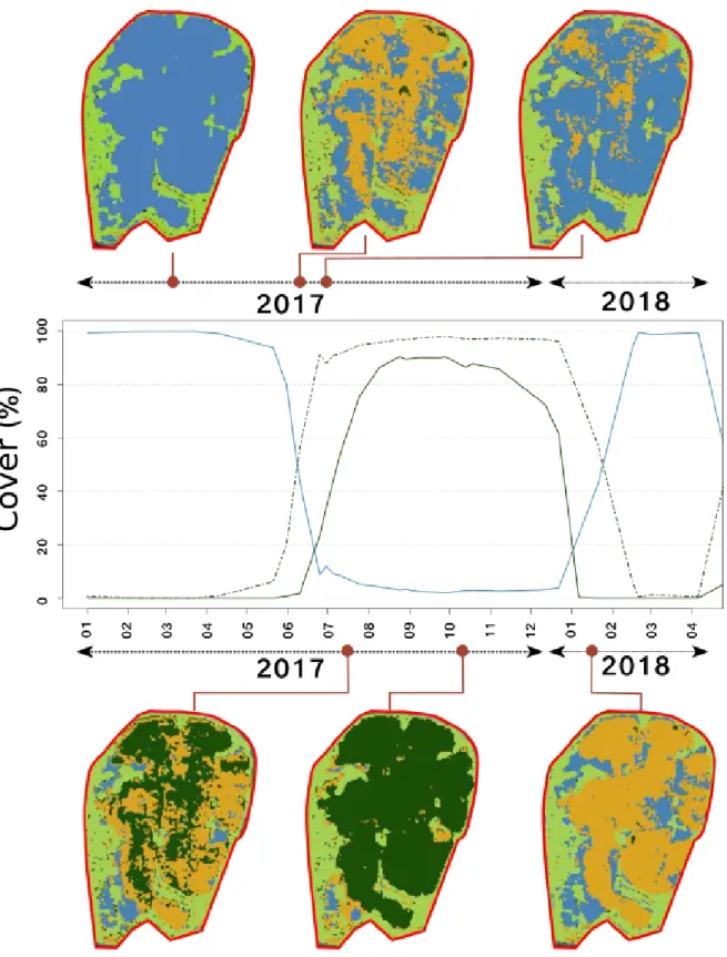
The threshold method is efficient in classifying in a discrete way (W, M, G) the aquatic vegetation over time. We choose to represent the results at 6 distinct dates representative of the seasonal variations of aquatic vegetation development (Figure 4). The results of the method are consistent in the sense that each pixel changes class over time in the way it should do following the vegetation annual cycle : from W to M (first stage of growth in the water) to G (maximum growth), then to M again (start of senescence phase) to W finally. The classified maps allow computing the relative areas of the different classes on a single graph. Adding the M and G class areas allows computing the global growth starting early spring 2017 and leading to the maximal extent at the end of August 2017, which is persistent over the whole lagoon until early January 2018. Senescence then starts and continues until the end of February 2018, where the lagoon is void of vegetation again. The mixed-phase corresponds indeed to submerged aquatic vegetation, and its dynamics allows detecting the very early stage of growth of aquatic vegetation. M area shows a peak in early July, corresponding to aquatic grass reaching the surface after the subaquatic development phase. Since floating aquatic vegetation reflects a radiometric signal different from submerged aquatic vegetation, it is then classified as G. At this transition time, the M area starts to grow, whereas the G area starts to decrease.
343 344 345 346 347 348 349 350 351 352 353 354 355 356 357 358 359 360 361 362 363 364 365 366 367 368 369 370 371
Figure 4: Classified maps obtained from the threshold method: W (blue), M (orange), G (dark green), reedbeds (light green). The blue line represents the water coverage over time, whereas the dark green line is the G coverage and the dashed dark green line is the (G+M) coverage.
373 374 375 376 377 378
3. Results using the Spectral Linear Unmixing (SLU) method
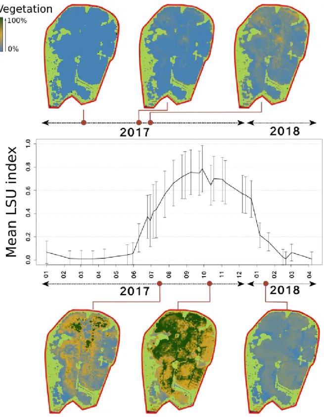
This method provides a continuous measure of the aquatic vegetation development over time, which is presumably proportional to an abundance measure. The dynamics of each pixel of the studied area is also consistent with the annual vegetation cycle. Figure 5 illustrates how pixels are analyzed using the SLU method and provide maps of a measure of vegetation abundance over time. The mean LSU index over variable pixels sums up the seasonal growth and senesence of the grassbeds. Photo-interpreted pixels of W, early G, and late G (see Appendix 4) are distinct from each other regarding aquatic vegetation content during the growth phase, and their maximum vegetation content during the summer and fall are also significantly different (not shown). However, they follow the same mortality curve during the senescence phase starting in December 2017. Water pixels are somehow analyzed in an unexpected way, with 40% of aquatic vegetation at the end of the fall, which may correspond (as it is most likely an artefact of the LSU method) to nutrient-rich content – either algal bloom or dying aquatic vegetation-(not shown).
379 380 381 382 383 384 385 386 387 388 389 390 391 392 393 394
Figure 5: Classified maps obtained from the LSU method: W (blue), M (orange), G (dark green), reedbeds (light green). The black curve is the mean LSU index temporal profile.
4. Comparison of the two methods
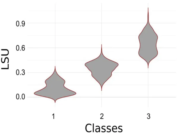
The two approaches are globally coherent, as we observed the expected trend of higher SLU values in the grass bed category compared to mixed and water. We observed a clear shift 396 397 398 399 400 401 402
between grass bed (G) and mixed (M) compartment for a SLU value of approximately 0.45. However, this limit is not perfectly clear between mixed (M) and water (W), as an overlap appeared for SLU values of 0.15 to 0.3. (Figure 6).
Figure 6: Comparison of the concordance of two modelling approaches (Linear Spectral Unmixing and Classification) to classify Sentinel 2 images into ecosystem compartments in a coastal lagoon. Violin plots represent the distribution of pixels value based on the LSU model (y-axis) classified in their related category (x-axis). Categories represent the three ecosystem compartments: 1 is for water, 2 is for mixed vegetation, and 3 is for grass bed.
5. Comparison with field data
To analyze the relationship between the proportion of categorized pixels through our remote sensing approach and the field estimate of grass bed abundance, we ran one test per category (Figure 7). For W, the proportion of pixels decreased significantly with the increase of grass bed abundance (coefficient estimate ~ -5.5 (±1.98), t-value ~ -2.781, p-value ~0.006) as expected. For G, the proportion of pixels increased significantly with the increase of grass bed abundance (coefficient estimate ~ 2.84 (±0.47), t-value ~ 6.041, p-value ~1.7e-08) as expected. For M, we detected a weak decrease in the proportion of pixels against grass bed abundance (coefficient estimate ~ -0.96 (±0.42), t-value ~ -2.284, p-value ~0.02) but no peak as previously expected. Such results have to be considered with care because both models performed poorly, as reflected in high overdispersion rate found for each one (residual deviance of 225, 684 and 695 for 112 degrees of freedom, for W, M, and G, respectively), 403 404 405 406 407 409 410 411 412 413 414 415 416 417 418 419 420 421 422 423 424 425 426 427 428
despite the use of quasi-binomial probability density functions. This failure is explained by the very high skewness toward high values of field data, as presented in Appendix 5.
We faced similar issues when running the comparison with LSU. We detected a significant positive relationship between field estimates of grass bed abundance and LSU (coefficient estimate ~ 7.02 (±1.04), t-value ~ 6.77, p-value ~5.02e-10). However, the model performed poorly as the residual deviance was 5405 on 121 degrees of freedom, which reflects very important overdispersion in data.
Figure 7: Comparison plot of field values with results from two modelling approaches (Linear Spectral Unmixing and Classification). Field samples were geolocalized, and the nine 10*10m pixels were attributed to the sampling station in order to account for GPS precision. The top three plots represent the proportion of pixels attributed to each class (plot a: water, b: mixed vegetation, c: grass bed) as a function of the cover of grass bed estimated through a field approach. The bottom plot (d) represent the proportion of grass 429 430 431 432 433 434 435 437 438 439 440 441 442 443 444 445 446 447
Discussion
Creating reliable ecological indicators is a prerequisite to assess the efficiency of ecosystem management. Lagoons are dynamic ecosystems of high conservation value, and monitoring grass bed is paramount to understanding their ecological status. Here we present an easy-to-handle method that allows managers to survey grass bed development every week based on the open, free and public satellites image archive of Sentinel-2. This tool allows reserve managers to survey vegetation at a high spatio-temporal resolution without any intrusion in the habitat (a crucial aspect in reserves), which limits disturbances of the ecosystem. The annual dynamics derived by this method and is a prerequisite knowledge to understand the grassbeds ecosystems over many years, given that it continues to be derived each year.
Spatial and temporal dynamic of pondweed grass beds of the Bagnas lagoon
Analyzing the spatial and temporal dynamics of vegetation every week has shed light on ecosystem dynamics that were hardly approached before (Antunes et al., 2012). In our case, satellite images were spread during one vegetative year; we detected a late growth by May and June. This could be due to the management drought generated the previous year (i.e.,
assec in French) to mineralize the substrate and limit eutrophication. Such perturbation could
have delayed the growth of pondweed and might have extirpated a fraction of the population. However, previous experiences had shown that most rhizomes remained alive, and individuals resprouted when water filled up the lagoon (but see also Casagranda and Boudouresque, 2007). This growth was followed by a maximum coverage reached in early August when the grass bed covered nearly the whole of the water body. Due to summer evaporation and high density of plants, leaves outcropped at the surface. The grass bed remained in a similar development state until winter when it slightly decreased. Finally, we did not detect any living vegetation during the two coldest months of 2018 winter (January-February). However, not detecting the vegetation is not equivalent to the death of individuals; it's probable that rhizomes have persisted in the substrate, while leaves died out and decomposed (Casagranda and Boudouresque, 2007; Van Wijk, 1988).
The extent of the grass bed cover is to be compared with past information, although no formal survey has produced analyzable data. In the early 1990s, the lagoon already contained a pondweed grass bed, but it was fragmented and patchy. After 10 years, the grass bed covered most of the water body during summer, and despite some inter-annual variability, it remained like this until now. S. pectinata is a halotolerant species whose growth increases under eutrophic conditions. Thus, its dominance reveals a high trophic state of the lagoon (Casagranda and Boudouresque, 2007; Menéndez López and Comín, 1989; Shili et al., 2007), which could have accumulated nutrients (i.e. nutrient sink, Rodrigo et al., 2013) due to small water inputs and a “saline effect” (i.e. nutrient accumulation after summer evaporation), though some purges are done in the winter and spring in the context of water level management (Agbarin et al., 2018). The management drought organized every 5 to 10 years aims at limiting eutrophication by mineralizing the substrate, but it is difficult to assess its efficiency because of a lack of precise surveys. Furthermore, a reflection is currently underway by the natural reserve scientific board to move towards a more passive management of the Bagnas lagoon, which should lead to an increase in water salinity (Agbanrin, 2018). 448 449 450 451 452 453 454 455 456 457 458 459 460 461 462 463 464 465 466 467 468 469 470 471 472 473 474 475 476 477 478 479 480 481 482 483 484 485 486 487 488 489 490 491 492 493
This change in ecological conditions may affect grass bed composition and spatial extent. Such changes will have to be monitored; therefore, the use of satellite images will constitute a fundamental tool to understand grass bed response to lagoon management and its overall impact on vegetation ecosystems.
A step toward a long-term automated survey of vegetations for conservation
The setting of long-term surveys within protected and managed natural areas is an essential step toward efficient conservation of ecosystems over time. Such surveys need to match several criteria, among which reproducibility (independence of observer), producing analyzable data (good statistical power), and low cost are crucial (David, 2005). Such constraints are even more stringent when quantifying dynamic processes require frequent resampling over the year. Thus, our approach is free of observer bias and produces two complementary perspectives of lagoon grass beds over time. These two classification methods are complementary, and both have their strengths and limits. The threshold method produces very stable results through time; however, thresholds are applied subjectively, and their strength should be assessed. On the other hand, the SLU method produced results that can be temporally a bit less coherent: subtle variation in plant growth, or changes in water level, can affect the reflectance of pixels and modify the calculated vegetation index. The value of endmembers used to calibrate the algorithm can in principle influence the estimate per pixel. The 42 pixels of water and 52 pixels of vegetation sampled as end members were selected in a homogeneous way across the lagoon (hence for different depths and different distances from the reedbeds borders) and spanning 17 satellite images over time. By analyzing reflectance values of the pixels for the 4 main bands (RGB and NIR) we noted that their distribution across pixels could be considered as narrow gaussians. For example, the mean NIR band reflectance for vegetation endmembers has 0.2176 mean value and 0.0419 standard deviation. This is somehow consistent with what is expected for « pure » endmembers. However, this has to be kept in mind and might not be always the case for further uses of « pure » endmembers across the years or for other lagoons More complex algorithms (such as Spectral
nonlinear unmixing) might also provide better results. However, the complementarity of the
two methods allows users to select the most adapted metric to their context. Additionally, it is worth mentioning that this methods could be tested using other spectral information, such as the red-edge region, where the vegetation reflectance generally increases (Shuster et al., 2012). The use of the red-edge NDVI index could lead to more refined classification depending on the context, as shown by Khanna et al. (2011) to distinguish macrophytes in turbid water; however this study based on plane-embarked hyperspectral tools cannot be reproduced with a frequency comparable to Sentinel-2 data. Note also that in the study of intertidal grassbeds of (Zoffoli et al, 2020), the NDVI index was proved to be sufficient for classification, which is probably due to the very low amount of water present at low tide and to the fact that no other vegetation seemed to be present. It could be interesting to test the validity of the MSAVI2 index that we used here in the context of intertidal grassbeds.
The integration of remote sensing-based surveys into conservation practices strongly relies on the use of simple methods, as overwhelming statistical complexity is one of the main breaks of knowledge transfer from research to applied conservation (Sutherland et al., 2019, 2009). Both methods presented here rely on very simple photointerpretation and basic knowledge of the lagoon to produce reliable results. The weak correlation observed with field data points out the weakness of field campaigns to survey such vegetative ecosystems; in 494 495 496 497 498 499 500 501 502 503 504 505 506 507 508 509 510 511 512 513 514 515 516 517 518 519 520 521 522 523 524 525 526 527 528 529 530 531 532 533 534 535 536 537 538 539
particular, the inaccuracy of field estimates to precisely quantify abundance within patches of high plant density. Non-intrusive estimates realized by sighting alone had a marked tendency to group all patches of high plant density, which led to an extreme skewness in our field data, and ultimately did not allow us to fit a representative model. Such skewness also prevented us from using supervised classification methods. Additionally, localization (due to the boat moving or drifting while sampling, for example) could have implied critical bias when further mapping results.
Yet, it is essential to mention that remote sensing-based maps represent the interpretation of a vegetation index based on the chlorophyllous activity of plants, which is not directly related to the abundance or the density of the plant. For example, pixels classified as mixed by the threshold method can represent sparse grass bed, dense grass bed but small plants with more water to the surface, or transition areas between grass bed and bare soil. Additionally, there is no consensus to link such vegetation index to a particular feature of vegetation, be it stem density or biomass (Vis et al., 2003).
Transferability assessment of the method
The Bagnas lagoon has constituted an appropriate training site to develop the method, as it allowed a precise detection of the grass bed through satellite images. However, the use of this method in different ecological contexts might require precautions before interpreting grass bed dynamics. First, the pondweed grass bed of the Bagnas lagoon was highly abundant and well developed, which allowed satellites to detect a clear photosynthetic signal. Sparse aquatic vegetation might be more complex to model (Ahmed et al., 2009). Then, the grass bed was dominated by one single species, which discarded any bias regarding different reflectance associated with different species. Regarding the structure of the water body, the lagoon is homogenously shallow (about 50cm in summer), which limits the impact of water to weaken the signal. Water was relatively clear, probably as a result of shallow water, high plant density that limits current and water column that contained little to no suspended sediment (Grillas et al., 2018; Shili et al., 2007). Finally, no micro-algae bloom occurred during the study period, an event than can blur the detection of grass bed by increasing the chlorophytic signal. Therefore, it is likely that the transferability of our approach might require some technical adaptations to be efficient in different contexts; for example, temporal series of images could be used to model a pixel-based vegetation index trajectory that could smooth measurement artifacts.
Perspectives to understand intra-annual and inter-annual plant growth or persistence
The rise of new ecological data opens new paths to model dynamics at a fine scale. Maps produced by the SLU method can be used to infer growth parameters (not measurable by field surveys) that are likely to be heterogeneous in space and likely to depend on the topographic and environmental parameters of the study site. Population dynamics simulations can be implemented using these parameters for prediction and management purposes in different environmental scenarios. This will provide temporal scenarios of plant coverage based on real data, to be compared to known theoretical cases where the effect of heterogeneity of growth rates (Hiebeler 2004) and connectivity heterogeneity (Gillaranz et al 2012, Huth et al 2015) have been previously studied. The Sentinel-2 image acquisition is expected to last to last until 2029 (with the potential launch of a complementary twin-satellite system in 2022) and will allow sustaining the intra-annual data analysis over several seasons 540 541 542 543 544 545 546 547 548 549 550 551 552 553 554 555 556 557 558 559 560 561 562 563 564 565 566 567 568 569 570 571 572 573 574 575 576 577 578 579 580 581 582 583 584 585
(work in progress). Hence the evolution of the vegetation year after year at its maximum development will be inferred. Hopefully, one will be able to learn from these data and their correlations with environmental parameters to build predictive models. Other detectors will be complementary for interannual monitoring such as Rapid Eye, in which archive data were used in Traganos and Reinartz (2018) in the study of Posidonia grass beds.
Conclusion
In this article, we have presented an off-the-shelf method combining ecological knowledge and open access remote-sensing technology to monitor the spatial extent of grass beds in shallow water lagoons over time, with a spatial resolution of 10m and a temporal frequency of 5 days. The multispectral data are available through the Copernicus Sentinel-2 program, but other detectors could also be used for local peculiarities. Hyperspectral detectors have been used for wetlands previously, and the linear spectral unmixing analysis method proposed here is also used in the hyperspectral context (Khanna et al., 2011, Bioucas-Dias et al., 2013) when different vegetation species may need to be distinguished. Missions using hyperspectral detectors will be more frequent in the future thanks to recent research and development efforts. We can cite missions in progress such as PRISMA (ASI), DESIS (DLR) , in preparation such as EnMAP (DLR) and finally in longer term preparation such as BG (NASA) and CHIME (ESA).Field survey analysis remains compulsory and is all the more useful as field campaign dates correspond to image acquisition dates, and the resolution scales are comparable. In the long term, the continuous survey of the grass beds at a particular location will allow understanding correlations between water quality, abiotic parameters, human activity, topography, and biodiversity. Online applications that allow anyone, from reserve managers to the general public, to follow the system, can be developed easily as is being done for the Bagnas lagoon training site (vegmap.irstea.fr).
Acknowledgments
We thank the staff of the National Natural Reserve of the Bagnas and ADENA for sharing their knowledge of the reserve, in particular Nathalie Guénel and Julie Bertrand. We thank Jean-Baptiste Féret, Kenji Ose, Dino Ienco, Marine Le Louarn for insightful discussions on the topic. Susan Ustin, Shruti Khanna from UC Davis, and Kathy Boyer from SFU in Tiburon provided insightful information on grass beds monitoring and remote-sensing techniques. We thank Benjamin Commandré for his efforts to make the results of this work accessible on a webmapping site under development. MM was supported by a grant from Agence de l'Eau ("appel a projet Biodiversité 2016"), which also served to finance field surveys. EP wants to thank the University of Montpellier and LabeX NUMEV through contract AAP2017-1-08. This research benefited from the support and services of UC Berkeley's Geospatial Innovation Facility (GIF, gif.berkeley.edu).
Author contributions
Menu Marion: data curation, analysis, and writing. Papuga Guillaume: fieldwork, data analysis and writing. Andrieu Frédéric: field work. Debarros Guilhem : visualization. Fortuny Xavier: writing. Alleaume Samuel: project administration and writing. Pitard Estelle : conceptualization, supervision, funding acquisition, data analysis, writing. All authors have reviewed & edited the draft.
586 587 588 589 590 591 592 593 594 595 596 597 598 599 600 601 602 603 604 605 606 607 608 609 610 611 612 613 614 615 616 617 618 619 620 621 622 623 624 625 626 627 628 629 630
References
Agbanrin, Y., 2018. Gestion hydraulique de la réserve naturelle du Bagnas (Stage ingénieur). Ecole Polytechnique, Montpellier.
Ahmed, M.H., El Leithy, B.M., Thompson, J.R., Flower, R.J., Ramdani, M., Ayache, F., Hassan, S.M., 2009. Application of remote sensing to site characterisation and environmental change analysis of North African coastal lagoons. Hydrobiologia 622, 147–171. https://doi.org/10.1007/s10750-008-9682-8
Antunes, C., Correia, O., Marques da Silva, J., Cruces, A., Freitas, M. da C., Branquinho, C., 2012. Factors involved in spatiotemporal dynamics of submerged macrophytes in a Portuguese coastal lagoon under Mediterranean climate. Estuarine, Coastal and Shelf Science 110, 93–100. https://doi.org/10.1016/j.ecss.2012.03.034
Arzel, C., Elmberg, J., Guillemain, M., 2006. Ecology of spring-migrating Anatidae: a review. Journal of Ornithology 147, 167–184.
Benedetti-Cecchi, L., Rindi, F., Bertocci, I., Bulleri, F., Cinelli, F., 2001. Spatial variation in development of epibenthic assemblages in a coastal lagoon. Estuarine, Coastal and Shelf Science 52, 659–668.
Bioucas-Dias, Jose & Plaza, Antonio & Camps-Valls, Gustau & Scheunders, Paul & Nasrabadi, N.M. & Chanussot, Jocelyn. (2013). Hyperspectral Remote Sensing Data Analysis and Future Challenges. Geoscience and Remote Sensing Magazine, IEEE. 1. 6-36. 10.1109/MGRS.2013.2244672.
Bradley, D., Thayer, S., Stentz, A., Rander, P., 2004. Vegetation detection for mobile robot navigation. Robotics Institute, Carnegie Mellon University, Pittsburgh, PA, Tech. Rep. CMU-RI-TR-04-12.
Camacho, A., Peinado, R., Santamans, A.C., Picazo, A., 2012. Functional ecological patterns and the effect of anthropogenic disturbances on a recently restored Mediterranean coastal lagoon. Needs for a sustainable restoration. Estuarine, Coastal and Shelf Science 114, 105–117. https://doi.org/10.1016/j.ecss.2012.04.034
Cañedo-Argüelles, M., Rieradevall, M., Farrés-Corell, R., Newton, A., 2012. Annual characterisation of four Mediterranean coastal lagoons subjected to intense human activity. Estuarine, Coastal and Shelf Science, Research and Management for the c o n s e r v a t i o n o f c o a s t a l l a g o o n e c o s y s t e m s 1 1 4 , 5 9 – 6 9 . https://doi.org/10.1016/j.ecss.2011.07.017
Casagranda, C., Boudouresque, C.F., 2007. Biomass of Ruppia cirrhosa and Potamogeton pectinatus in a Mediterranean brackish lagoon, Lake Ichkeul, Tunisia. Fundamental and Applied Limnology 168, 243–255. https://doi.org/10.1127/1863-9135/2007/0168-0243 Cazals, C., Rapinel, S., Frison, P.-L., Bonis, A., Mercier, G., Mallet, C., Corgne, S., Rudant,
J.-P., 2016. Mapping and characterization of hydrological dynamics in a coastal marsh using high temporal resolution Sentinel-1A images. Remote Sensing 8, 570. https://doi.org/10.3390/rs8070570
Chave, P., 2001. The EU Water Framework Directive. IWA Publishing.
David, H., 2005. Handbook of biodiversity methods: survey, evaluation and monitoring. Cambridge University Press.
Duarte, P., Bernardo, J.M., Costa, A.M., Macedo, F., Calado, G., Cancela da Fonseca, L., 2002. Analysis of coastal lagoon metabolism as a basis for management. Aquatic Ecology 36, 3–19. https://doi.org/10.1023/A:1013394521627 631 632 633 634 635 636 637 638 639 640 641 642 643 644 645 646 647 648 649 650 651 652 653 654 655 656 657 658 659 660 661 662 663 664 665 666 667 668 669 670 671 672 673 674 675 676
Gaertner-Mazouni, N., De Wit, R., 2012. Exploring new issues for coastal lagoons monitoring and m an age m ent . Est ua ri ne , C oa sta l an d Sh el f Sc i en ce 11 4, 1–6. https://doi.org/10.1016/j.ecss.2012.07.008
Gardner, R.C., Davidson, N.C., 2011. The Ramsar convention, in: LePage, B.A. (Ed.), Wetlands: Integrating Multidisciplinary Concepts. Springer Netherlands, Dordrecht, pp. 189–203. https://doi.org/10.1007/978-94-007-0551-7_11
GDAL/OGR contributors (2020). GDAL/OGR Geospatial Data Abstraction software Library. Open Source Geospatial Foundation. URL https://gdal.org
Gillaranz, L.J, Bascompte, 2012. J. Spatial network structure and metapopulation persistence. Journal of Theoretical Biology, 297, 11-16.
Grillas, P., Hilaire, S., Fontès, H., Bec, B., 2018. Campagne de surveillance 2017 de l’état DCE des lagunes méditerranéennes oligo-et mésohalines françaises pour la physico-chimie, le phytoplancton et les macrophytes. Consolidation de l’indicateur macrophytes. Bilan des résultats 2017 (Research Report). Institut de recherche de la Tour du Valat ; Agence de l’eau Rhône-Méditerranée-Corse 79p.
Hagolle, O., Huc, M., Desjardins, C., Auer, S., Richter, R., 2017. MAJA algorithm theoretical basis document. https://doi.org/10.5281/zenodo.1209633
Harrell Jr, F.E., 2018. Hmisc: Harrell miscellaneous (Version 4.1-1). Vanderbilt University. Hartog, C., 1981. Aquatic plant communities of poikilosaline waters. Hydrobiologia 81, 15–
22.
Hiebeler, D., 2004. Competition between far and near disperserd in spatially structured habitats. Theoretical Population Biology 66, 205-218.
Holm, T.E., Clausen, P., 2006. Effects of water level management on autumn staging waterbird and macrophyte diversity in three danish coastal lagoons. Biodiversity and Conservation 15, 4399–4423. https://doi.org/10.1007/s10531-005-4384-2
Huth, G., Haegeman, B., Pitard, E., Munoz, F., 2015. Long-distance rescue and slow extinction dynamics govern multiscale metapopulations. The American Naturalist 186, 460.
Keshava, N., Mustard, J.F., 2002. Spectral unmixing. IEEE signal processing magazine 19, 44–57.
Khanna, S., Santos, M.J., Ustin, S.L., Haverkamp, P.J., 2011. An integrated approach to a biophysiologically based classification of floating aquatic macrophytes. International Journal of Remote Sensing 32, 1067–1094.
Kohlus, J., Stelzer, K., Müller, G., Smollich, S., 2020, Mapping seagrass (Zostera) by remote sensing in the Schleswig-Holstein Wadden Sea. Eastuarine, Coastal and Shelf Science 238, 106699.
Lehmann, A., Lachavanne, J.-B., 1997. Geographic information systems and remote sensing in aquatic botany. Aquatic Botany 3, 195–207.
Lloret, J., Marín, A., 2009. The role of benthic macrophytes and their associated macroinvertebrate community in coastal lagoon resistance to eutrophication. Marine Pollution Bulletin 58, 1827–1834.
Lyons, M.B., Roelfsema, C.M., Phinn, S.R., 2013. Towards understanding temporal and spatial dynamics of seagrass landscapes using time-series remote sensing. Estuarine, Coastal and Shelf Science 120, 42–53.
677 678 679 680 681 682 683 684 685 686 687 688 689 690 691 692 693 694 695 696 697 698 699 700 701 702 703 704 705 706 707 708 709 710 711 712 713 714 715 716 717 718 719 720
Menéndez López, M., Comín, F.A. (Francisco A.), 1989. Seasonal patterns op biomass variation of Ruppia cirrhosa (Petagna) Grande and Potamageton pectinatus L. in a coastal logoon. Scientia Marina 53, 633-638.
Newton, A., Brito, A.C., Icely, J.D., Derolez, V., Clara, I., Angus, S., Schernewski, G., Inácio, M., Lillebø, A.I., Sousa, A.I., Béjaoui, B., Solidoro, C., Tosic, M., Cañedo-Argüelles, M., Yamamuro, M., Reizopoulou, S., Tseng, H.-C., Canu, D., Roselli, L., Maanan, M., Cristina, S., Ruiz-Fernández, A.C., Lima, R.F. de, Kjerfve, B., Rubio-Cisneros, N., Pérez-Ruzafa, A., Marcos, C., Pastres, R., Pranovi, F., Snoussi, M., Turpie, J., Tuchkovenko, Y., Dyack, B., Brookes, J., Povilanskas, R., Khokhlov, V., 2018. Assessing, quantifying and valuing the ecosystem services of coastal lagoons. Journal for Nature Conservation 44, 50–65. https://doi.org/10.1016/j.jnc.2018.02.009 Obrador, B., Pretus, J.L., 2010. Spatiotemporal dynamics of submerged macrophytes in a
Mediterranean coastal lagoon. Estuarine, Coastal and Shelf Science 87, 145–155. https://doi.org/10.1016/j.ecss.2010.01.004
Pereira, P., De Pablo, H., Vale, C., Franco, V., Nogueira, M., 2009. Spatial and seasonal variation of water quality in an impacted coastal lagoon (Óbidos Lagoon, Portugal). Environmental monitoring and assessment 153, 281–292.
Pérez-Ruzafa, A., Marcos, C., Pérez-Ruzafa, I.M., Pérez-Marcos, M., 2011. Coastal lagoons: “transitional ecosystems” between transitional and coastal waters. Journal for Coastal Conservation 15, 369–392. https://doi.org/10.1007/s11852-010-0095-2
Pojana, G., Gomiero, A., Jonkers, N., Marcomini, A., 2007. Natural and synthetic endocrine disrupting compounds (EDCs) in water, sediment and biota of a coastal lagoon. Environment International 33, 929–936.
Qi, J., Chehbouni, A., Huerte, A.R., Kerr, Y.H., Sorooshian, S., 1994. A modified soil adjusted vegetation index. Remote Sensing Environment 48, 119–126.
R Core Team (2019). R: A language and environment for statistical computing. R Foundation for Statistical Computing, Vienna, Austria. URL https://www.R-project.org/.
Rodrigo, M.A., Martín, M., Rojo, C., Gargallo, S., Segura, M., Oliver, N., 2013. The role of eutrophication reduction of two small man-made mediterranean lagoons in the context of a broader remediation system: Effects on water quality and plankton contribution. Ecological Engineering 61, 371–382. https://doi.org/10.1016/j.ecoleng.2013.09.038 Santos, M.J., Khanna, S., Hestir, E.L., Greenberg, J.A., Ustin, S.L., 2016. Measuring
landscape-scale spread and persistence of an invaded submerged plant community from airborne remote sensing. Ecological applications 26, 1733–1744.
Scheffer, M., 1997. Ecology of shallow lakes. Springer Science & Business Media.
Schuster, C., Förster, M., Kleinschmit, B., 2012. Testing the red edge channel for improving land-use classifications based on high-resolution multi-spectral satellite data. I n t e r n a t i o n a l J o u r n a l o f R e m o t e S e n s i n g 3 3 , 5 5 8 3 – 5 5 9 9 . https://doi.org/10.1080/01431161.2012.666812
Shili, A., Maïz, N.B., Boudouresque, C.F., Trabelsi, E.B., 2007. Abrupt changes in Potamogeton and Ruppia beds in a Mediterranean lagoon. Aquatic Botany 87, 181–188. https://doi.org/10.1016/j.aquabot.2007.03.010
Silva, T.S.F., Costa, M.P.F., Melack, J.M., Novo, E.M.L.M., 2008. Remote sensing of aquatic vegetation: theory and applications. Environmental monitoring and assessment 140, 131–145. https://doi.org/10.1007/s10661-007-9855-3 721 722 723 724 725 726 727 728 729 730 731 732 733 734 735 736 737 738 739 740 741 742 743 744 745 746 747 748 749 750 751 752 753 754 755 756 757 758 759 760 761 762 763 764 765
Sutherland, W.J., Adams, W.M., Aronson, R.B., Aveling, R., Blackburn, T.M., Broad, S., Ceballos, G., Cote, I.M., Cowling, R.M., Da Fonseca, G.A.B., 2009. One hundred questions of importance to the conservation of global biological diversity. Conservation Biology 23, 557–567.
Sutherland, W.J., Fleishman, E., Clout, M., Gibbons, D.W., Lickorish, F., Peck, L.S., Pretty, J., Spalding, M., Ockendon, N., 2019. Ten years on: a review of the first global conservation horizon scan. Trends in Ecology & Evolution 34, 139-153. https://doi.org/10.1016/j.tree.2018.12.003
Therville, C., Mathevet, R., Bioret, F., 2012. Des clichés protectionnistes aux discours intégrateurs: l’institutionnalisation de réserves naturelles de France. VertigO 12:24. Traganos, D., Reinartz, P., 2018. Interannual change detection of mediterranean seagrasses
using rapidEye image time series. Frontiers in Plant Science 9, 96. https://doi.org/10.3389/fpls.2018.00096
Traganos, D., Reinartz, P., 2018. Mapping Mediterranean seagrasses with Sentinel-2 imagery. Marine Poluution Bulletin 134, 197-209.
Van der Maarel, E. (1979). Transformation of cover-abundance values in phytosociology and its effects on community similarity. Vegetatio, 39(2), 97-114.
Van Wijk, R.J., 1988. Ecological studies on Potamogeton pectinatus L. I. General characteristics, biomass production and life cycles under field conditions. Aquatic Botany 31, 211–258. https://doi.org/10.1016/0304-3770(88)90015-0
Veetil,B.K., Ward, R.D., Do Amaral Camara Lima M., Stankovic., M., Hoai P.N., Quang N.X., 2020, Opportunities for seagrass research derived from remote sensing: A review of current methods, Ecological Indicators, 117, 106560.
Vis, C., Hudon, C., Carignan, R., 2003. An evaluation of approaches used to determine the distribution and biomass of emergent and submerged aquatic macrophytes over large spatial scales. Aquatic Botany 77, 187–201. https://doi.org/10.1016/S0304-3770(03)00105-0
Wikantika, K., Uchida, S., Yamamoto, Y., 2002. Mapping vegetable area with spectral mixture analysis of the Landsat-ETM, in: IEEE International Geoscience and Remote Sensing Symposium. IEEE, pp. 1965–1967.
Yamamuro, M., 2012. Herbicide-induced macrophyte-to-phytoplankton shifts in Japanese lagoons during the last 50 years: consequences for ecosystem services and fisheries. Hydrobiologia 699, 5–19. https://doi.org/10.1007/s10750-012-1150-9
Zoffoli M.L., Gernez P., Rosa P., Le Bris A., Brando V.E., Barillé A-L., Harin, N, Petrs S, Poser K., Spaias., Peralta., Barillé, 2020, Remote Sensing of Environment, 251, 112020. 766 767 768 769 770 771 772 773 774 775 776 777 778 779 780 781 782 783 784 785 786 787 788 789 790 791 792 793 794 795 796 797 798 799 800 801 802