Applications of Missing Feature Theory to Speaker
Recognition
by
Michael Thomas Padilla
B.S., Electrical Engineering (1997)
University of California, San Diego
Submitted to the Department of Electrical Engineering and Computer
Science
in partial fulfillment of the requirements for the degree of
Master of Science in Electrical Engineering and Computer Science
at the
MASSACHUSETTS INSTITUTE OF TECHNOLOGY
February 2000
@
Massachusetts Institute of Technology 2000. All rights reserved.
Author
.- .. ... . . . .Department of Electrical Engineering and Computer Science
January 31, 2000
Certified by. 4...
Thomas F. Quatieri
SenipraStaf, MIT Lincoln Laboratory
> -4hqA Supprvisor
Accepted by...
Arthur C. Smith
Chairman, Department Committee on Graduate Students
This work was sponsored by the Department of the Air Force. Opinions, interpretations, conclusions, and recommendations are those of the author and not necessarily endorsed by
f CHUSETTSiNSTTITirF' the United States Air Force.
Applications of Missing Feature Theory to Speaker
Recognition
by
Michael Thomas Padilla
Submitted to the Department of Electrical Engineering and Computer Science on January 31, 2000, in partial fulfillment of the
requirements for the degree of
Master of Science in Electrical Engineering and Computer Science
Abstract
An important problem in speaker recognition is the degradation that occurs when speaker models trained with speech from one type of channel are used to score speech from another type of channel, known as channel mismatch. This thesis investigates various channel compensation techniques and approaches from missing feature theory for improving Gaussian mixture model (GMM)-based speaker verification under this mismatch condition. Experiments are performed using a speech corpus consisting of "clean" training speech and "dirty" test speech equal to the clean speech corrupted
by additive Gaussian noise. Channel compensation methods studied are cepstral
mean subtraction, RASTA, and spectral subtraction. Approaches to missing feature theory include missing feature compensation, which removes corrupted features, and missing feature restoration which predicts such features from neighboring features in both frequency and time. These methods are investigated both individually and in combination. In particular, missing feature compensation combined with spectral subtraction in the discrete Fourier transform domain significantly improves GMM speaker verification accuracy and outperforms all other methods examined in this thesis, reducing the equal error rate by about 10% more than other methods over a SNR range of 5-25 dB. Moreover, this considerably outperforms a state-of-the-art GMM recognizer for the mismatch application that combines missing feature the-ory with spectral subtraction developed in a mel-filter energy domain. Finally, the concept of missing restoration is explored. A novel linear minimum mean-squared-error missing feature estimator is derived and applied to pure vowels as well as a clean/dirty verification trial. While it does not improve performance in the verifica-tion trial, a large SNR improvement for features estimated for the pure vowel case indicate promise in the application of this method.
Thesis Supervisor: Thomas F. Quatieri Title: Senior Staff, MIT Lincoln Laboratory
Acknowledgments
I would like to foremost thank Tom Quatieri, my advisor and mentor, for allowing me to work with him as a research assistant and for always very graciously offering me his time and effort in guiding me along the way towards the completion of this thesis. It has truly been not only very educational, but also very enjoyable working with Tom. One of the most important things I've learned from Tom is the great value of creativity in research. Thank you very much.
I also sincerely thank Doug Reynolds and Jack McLaughlin for also always being there to offer me their time and invaluable comments and suggestions. I have a feeling that the mutual interest that Jack and I have in traveling may lead to us to meet unexpectedly at some far flung corner of the world someday. A big thank you also goes out to Cliff Weinstein and Marc Zissman for accepting me into the Lincoln Laboratory Group 62 and the US Air Force for offering the funding that made it all possible. I also thank the rest of the Group 62 members for their friendliness and for making the lab a very enjoyable working environment.
On a more personal note I thank all of my dear friends, both in the US and abroad, for all of their encouragement ever since I can remember. The joy their friendship has brought to my life has enhanced the academic side and made it all that much easier. Last, but certainly not least, I thank my family - my parents Manuel and Martha, my grandmother Laura ("Golden Oldie"), my uncle Steve, and all my other rela-tives scattered around the US for all of the love and support they have offered me throughout my life.
Contents
1 General Introduction 12
1.1 Introduction to Speaker Recognition . . . . 12
1.2 The GMM Speaker Recognition System . . . .. 14
1.3 Mel-Cepstrum and Mel-filter Energy Speech Features . . . . 19
1.4 The Speaker Mismatch Problem in Speaker Verification . . . . 21
1.5 Problem Addressed . . . . 22
1.6 Contribution of Thesis . . . . 25
1.7 Organization of Thesis . . . . 26
2 Channel Compensation and Techniques for Robust Speaker Recog-nition 28 2.1 Cepstral Mean Subtraction . . . . 30
2.2 RelAtive SpecTrA . . . . 32
2.2.1 Introduction and Basic System . . . . 32
2.2.2 Lin-Log RASTA . . . . 34
2.3 Delta Cepstral Coefficients . . . . 36
2.4 Results with TSID Corpus . . . . 37
3 Spectral Subtraction 40 3.1 Mel-Filter Energy Domain Spectral Subtraction . . . . 41
3.2 Soft |DFT Domain Spectral Subtraction . . . . 43
4 Missing Feature Theory 49
4.1 Missing Feature Theory . . . . 50
4.2 Missing Feature Compensation . . . . 50
4.3 Missing Feature Detection . . . . 56
4.4 Results for Missing Feature Compensation . . . . 59
5 Cascade Noise Handling Systems 65 5.1 RASTA with Spectral Subtraction . . . . 66
5.2 RASTA with Missing Feature Compensation . . . . 66
5.3
IDFT
Domain Spectral Subtraction with Missing Feature Compensation 69 5.4 RASTA with Spectral Subtraction and Missing Feature Compensation 69 6 Missing Feature Restoration 72 6.1 Previous Work in MFR . . . . 736.1.1 Integrated Speech-Background Model . . . . 73
6.1.2 Mean Estimation . . . . 74
6.1.3 R esults . . . . 75
6.2 Time-Frequency Linear Minimum Mean-Squared Error Missing Fea-ture Estim ation . . . . 75
6.3 Proposed System for Missing Feature Restoration . . . . 81
6.4 Results Using Linear MMSE Missing Feature Restoration . . . . 90
7 Conclusions 94 7.1 Summary of Thesis . . . . 94
List of Figures
1-1 Sample DET curve. . ... 14
1-2 Example: Distribution of features from states "A" and "B". . . . . 15
1-3 Graphical representation of speaker models. . . . . 17
1-4 Triangular Mel-Scale Filterbank. . . . . 20
1-5 Representative "clean" (top) and "dirty" (bottom) speech time-domain wave-forms from the TSID corpus. Both are from the same utterance. . . . . . 23
1-6 Representative "clean" (top) and "dirty" (bottom) speech spectrograms from the TSID corpus. Both are from the same utterance . . . . 23
1-7 DET curve showing error rate performance for baseline tests on TSID corpus. 24 2-1 The frequency response of the RASTA filter H(w). . . . . 33
2-2 The impulse response of the RASTA filter h[n]. . . . . 33
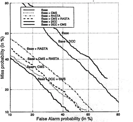
2-3 Comparison of various equalization techniques. . . . . 38
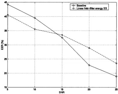
3-1 Plot showing EER vs. SNR (AWGN) for both the baseline case as well as with linear mel-filter energy domain spectral subtraction. It is seen that the performance relative to the baseline depends on the SNR of the additive noise, gains over baseline occuring at lower SNR levels. . . . . 47
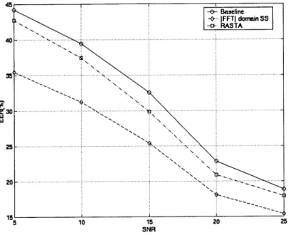
3-2 Plot showing EER vs. SNR (AWGN) for both the baseline case as well as with IDFT domain spectral subtraction. The application of spectral subtraction in this domain is seen to improve performance over the baseline case significantly at all SNR levels, going from about a 4% improvement at high SNRs to a near 10% improvement at low SNRs. For comparison, results for RASTA processing are also shown. . . . . 48
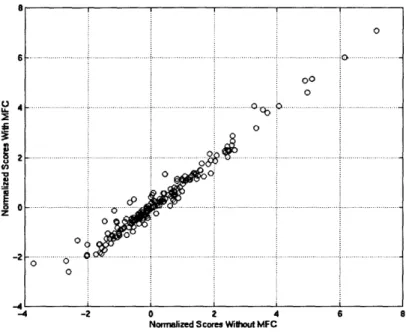
4-1 This plot shows the background model normalized log probability scores without MFC versus the corresponding values with MFC. The hope is that normalization of speakers' log probability scores with the background model's score will help to properly normalize the probability space in cases where MFC is applied. In this plot, the scores where MFC was applied resulted from removing the 1 0th feature from every frame. It is seen that
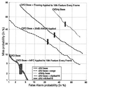
corresponding scores with and without MFC tend to be highly correlated, supporting the claim the background model normalization helps correct for improperly normalized pdf's when MFC is applied. Similar results were seen when slightly more features were removed in a controlled fashion as well. 54 4-2 Illustration of DET performance with 1 0th linear mel-filter energy feature
floored and with the same feature removed via MFC. MFC is seen to recover the baseline performance. DET curves with 20 dB of additive noise are given for reference. . . . . 55
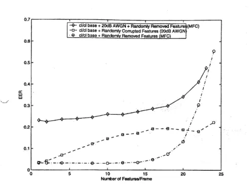
4-3 Trade-off between corrupted features and removing speech information in MFC. This curve shows EER performance with and without MFC for an increasing number of randomly corrupted or removed mel-energy features. 57
4-4 Average correlation between the perfect mf detector (a = 3.0) and
nonper-fect mf detectors (a = 1.0 and 3.0). Shows that the average correlation for
the a = 3.0 nonperfect detector is > 0.7 for most of the features, close to 0.9 for the highest ten features. The nonperfect detector with a = 1.0 has
been shown for reference. . . . . 60
4-5 Plot showing the average number a particular feature is declared missing per frame by the perfect mf detector(a = 3.0) and nonperfect mf detectors
(a = 1.0 and 3.0). The perfect and a = 3.0 nonperefect detectors are seen
4-6 Plot showing the frequency per frame that a given total number of missing features are detected by the perfect mf detector(a = 3.0) and nonperfect
mf detectors (a = 1.0 and 3.0). The results for the perfect and a = 3.0
nonperefect detectors are seen to be almost identical. Results are for 20 dB
AW GN . . . . . 62
4-7 EER vs. SNR for MFC with both perfect and nonperfect applications of MFC as well as the baseline case. Both the nonperfect and perfect missing feature detectors are shown to have nearly identical results at all SNR lev-els. At lower SNRs MFC is seen to degrade performance slightly (< 1%), while at higher SNR levels above approximately 17 dB it starts to improve performance by close to 3.5%. . . . . 64
5-1 EER performance as a function of SNR for cascade systems using RASTA
and one of linear mel-filter energy or |DFT| SS systems. For comparison the baseline system, the RASTA system, and the JDFTJ system are plotted as well. It is seen that when linear mel-filter energy SS is used with RASTA that performance is worse than straight RASTA at all SNR levels except than the lowest, at 5 dB. This is in contrast to the system using RASTA with |DFT SS, which is seen to do better than either RASTA or IDFT|
SS used alone at almost all SNRs. For this system EER performance is
typically 8% better than the baseline system. . . . . 67 5-2 Performance with a system combining RASTA with missing feature
com-pensation. Performance curves for the baseline and pure RASTA systems are shown for comparison. It is seen that the RASTA+MFC system un-derperforms both the baseline and pure RASTA systems, particularly the pure RASTA system. Only at high SNR levels of 20 dB and above are any benefits seen, but then only by about 1%. . . . . 68
5-3 Combination systems of IDFT domain SS + missing feature compensation and linear mel-filter energy SS + missing feature compensation. Also shown are the baseline and pure SS systems' performance for comparison. The
IDFT domain SS + MFC system substantially outperforms the linear mel-filter energy SS + MFC system as well as the other systems shown, at all SNR values. It is seen to perform better than the baseline system by approximately 15%. The linear mel-filter energy SS + MFC system, on the other hand, only achieves performance roughly halfway between these two. 70
5-4 RASTA processing in combination with missing feature compensation and linear mel-filter energy SS or IDFT domain SS. The system with the IDFT
domain SS is seen to do better than the other system as well as baseline for at all noise levels. The system with linear mel-filter energy SS only improves over the baseline at low SNR values, hurting performance at the higher ones. 71
6-1 3-Dimensional plot of linear mel-filter energy feature trajectories from a clean speech file. . . . . 82 6-2 3-Dimensional plot of logarithmic mel-filter energy feature trajectories from
a clean speech file. . . . . 83 6-3 Example clean linear mel-filter energy time trajectory. It is seen that the
waveform is far from random, having the property that features close in time tend to have similar values and a perceivable underlying deterministic nature. . . . . 83
6-4 Representative autocorrelation function for several linear mel-filter energy features. Speech is taken from a clean speech file. . . . . 84
6-5 Representative crosscorrelation function for several linear mel-filter energy features. Speech is taken from a clean speech file. . . . . 84
6-6 Representative autocorrelation function for several linear mel-filter energy features from a pure vowel (/E/). It is seen that the amount of autocorrela-tion for each trajectory is rather high, compared to the overall average. . . 86
6-7 Representative crosscorrelation function for several linear mel-filter energy
features and their neighbors from a pure vowel (/e/). It is seen that the amount of crosscorrelation for each trajectory is rather high, compared to the overall average. . . . . 86 6-8 Representative autocorrelation function for several linear mel-filter energy
features from a pure fricative (/f/). It is seen that the amount of autocor-relation for each trajectory is rather low, compared to the overall average and the pure vowel. . . . . 87 6-9 Representative crosscorrelation function for several linear mel-filter energy
features and their neighbors from a pure fricative (If/). It is seen that the amount of crosscorrelation for each trajectory is rather low, compared to the overall average and the pure vowel. . . . . 87 6-10 EER values for clean/dirty speaker verification task where missing features
are detected and replaced, when possible, by using the linear MMSE missing feature estimator. Performance is seen to degrade considerably in compari-son to the baseline case. . . . . 92
List of Tables
2.1 Results applying various channel compensation techniques to TSID data for train clean/test dirty case. . . . . 37 6.1 Results of applying proposed linear MMSE missing feature restoration
sys-tem to a pure vowel /e/. Columns indicate additive noise level, percentage of speech features declared to be missing out of all speech features, percent-age of features restored out of all speech features, the SNR of all features restored prior to restoration, and the SNR of all features restored after restoration. Results are for an artificially corrupted clean vowel recording. 91
Chapter 1
General Introduction
In this chapter the problem of speaker recognition is introduced along with various subareas of research and associated terminology. This leads into a description of the currently most commonly used statistical speaker model, the Gaussian mixture model, as well as the type of speech representation typically used by this model. Finally, the general problem addressed by this thesis is described.
1.1
Introduction to Speaker Recognition
The goal in speaker recognition is to recognize a person from his or her voice. Within this broad description are two specific problems: speaker identification and speaker
verification. Speaker identification attempts to associate an unknown voice with a
particular known voice taken from a known set of voices. Speaker verification, on the other hand, tries to determine if an unknown voice matches a particular known voice. The speech used for these tasks can be either a known phrase, termed
text-dependent, or can be a completely unconstrained phrase, termed text-independent.
Typical applications for speaker recognition are reconnaissance, forensics, access con-trol, automated telephone transactions, speech data management, etc.
Both speaker identification and speaker verification tasks can be thought of as consisting of two stages: training and testing. In training, the goal is to efficiently (in terms of both computational complexity as well as a minimum of information
redun-dancy) extract from the speech signal some values that represent characteristics that are as unique to that speaker as possible and contain very little of the environment's (the "channel") characteristics, since the acoustic environment in which the speech was recorded might otherwise be falsely included into the speaker models. While to humans the identity of the speaker of a given utterance appears through a complex combination of both high-level cues (such as semantics and diction), mid-level cues (such as prosodics), and low-level cues (such as the acoustic nature of the speech waveform including its frequency domain behavior, pitch, etc.), automatic speaker recognition systems have so far been unable to efficiently and effectively take advan-tage of any information other than low-level acoustic cues since these have been the easiest to automatically (without human supervision) extract and apply. The most commonly employed acoustic cues are spectral features such as formant trajectories, the resonant frequencies of the vocal tract, and the speaker's pitch.
In describing the performance of speaker ID and verification systems there are typically two types of error measures that are focused on. The first, the miss
prob-ability, represents the case where a true claimant, the speaker who is "claiming" to
have produced the test utterance, is incorrectly rejected by the system. The second error measure, the false acceptance probability, represents the case where an
impos-tor, a speaker who falsely claims to have produced the test utterance, is incorrectly
verified by the system as having produced the speech. The relative amounts of both types of errors that occur is determined by the threshold setting used in a maximum likelihood ratio test, which is applied in a manner similar to its use in detection prob-lems in digital communications theory. In a manner similar to how receiver operating characteristic curves are used in communications, in speaker verification problems
de-tection error trade-off (DET) curves are used in which false acceptance probabilities
are plotted versus miss probabilities for a wide range of possible threshold settings, indicating all the different operating points of the system that are achievable. While the overall behavior of DET curves is of interest, the equal error rate (ERR) point, where the two types of errors are equal, is often focused on as a good representative measure that does not bias the system towards a particular type of error in comparing
5 - Samp e. DE curve
60 A probabilit (in %)
F40 1-1: Sampl DET cue..
M
dfee se sycs. A example DET curve is given in.figure.1-1
-h 20M
5 2 0 2 4 os
In most modern speech systems, features are extracted from speech windowed with
a 20 ms window and the window is typically advanced at 10 ms intervals. To avoid
extracting features of the channel and its noise characteristics, it is essential that a speech detector be used to estimate and indicate which of the windowed frames
contain mostly speech and which contain mostly channel noise. For frames that
are labeled as speech, the system takes the windowed sfrm speerforms short-time
Fourier transform (STFT) based analysis on the segment. This is a filterbank analysis
which reduces the spectral representation, typically to the commonly employed
mel-cepstral coefficients, which will be described in the following section. Following this,
there will often be a channel equalization stage to mitigate the effect of the channel. Common equalization techniques, which will be described later, are RASTA and
p( FEATURE I A)
p( FEATURE 1 B)
- FEATURE
Figure 1-2: Example: Distribution of features from states "A" and "B".
cepstral mean subtraction.
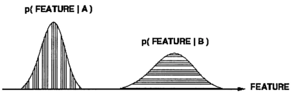
It is of interest how these speech features (typically mel-cepstral features) are associated with different speakers in a quantitative and statistical manner, allowing the construction of mathematical speaker models. In answering this question, speech researchers have depended on much of the work previously done in the area of statis-tical pattern recognition. Since the primary speaker-dependent acoustic information employed is taken from the spectrum reflecting vocal tract shapes, it is preferred to create speaker models that in some way capture those shapes as manifested in the speech features. To understand what approach is taken, assume that there are two states "A" and "B" (either distinct speakers or vocal tract states of a single speaker) and that each class produces features vectors with a certain probability distribution,
as shown in figure 1-2 1.
If we assume that the underlying distributions of the feature vectors in each class are Gaussian, then it is possible to train the model parameters of the underlying prob-ability density functions (pdf's) in an unsupervised manner not requiring any human supervision by using the expectation-maximization (EM) algorithm [10]. Using the state models, a new feature may be classified as follows
x is from state "A"
p(x|A) Z p(x|B),
x is from state "B"
assuming equally likely classes "A" and "B". It is thus seen that this is essentially a hypothesis testing problem.
In the statistical speaker model, the speaker is regarded as a random source pro-ducing the observed speech feature vectors X and it is the "state" that the speaker's vocal tract is in, as in the example using states A and B above, that determines the general distribution of these vectors. While it is understood that the probability of the speaker being in any one of the states describing his or her speech production mechanism nor that the transition probabilities between the different states is clearly not uniform, for computational ease an assumption of uniform state and state transi-tion probabilities is made. With this assumptransi-tion, it may be shown that the pdf of the observed speaker is a Gaussian mixture model (GMM)[10]. If an M-state statistical speaker is assumed, the resulting GMM speaker model is given by
M
p(XIA) = Ep ib(X)
i=1
where
b(X) = (27r)D/2IE.I1/2 exp-(X - pi )
-In the above expression ptL and EIj are the mean vector and covariance matrix for speaker state i, D is the dimensionality of the feature vectors, and pi is the probability of being in state i. Note that the set of quantities
A = (pi, pi, Ej), for i = 1,...,M
represents the parameters for each state of the speaker model for speaker A, and hence constitutes a speaker model. This concept is shown graphically in figure 1-3. It is thus observed that in this model the probability of the observed feature vector X from speaker model A is the sum of pdf's for each of the hidden and unknown states, appropriately weighted by the probability pi of the speaker being in that state. Given this resulting speaker model p(X|A), a quantitative score for the likelihood that an unknown feature vector was generated by a particular speaker may be calculated. The model parameter estimates (pi, pi, Ej), i=1,...,M are obtained by the EM algorithm
DOUG 1=(pi I,,)
Dour-__ _ _ __ _ _ __ M __a_ RBFLL _ _ _
ElOS RE E SP E F DELS:}MO
UTSERANCES MXURE ORDER ONE MODEL PER SPEAKER
Figure 1-3: Graphical representation of speaker models. mentioned earlier.
Although the speaker verification task requires only a binary decision of whether the claimant should be accepted or rejected, it is a more involved problem than the simple identification task[10]. This is a result of the fact that the class of "not speaker" is not very clearly defined. In the case of speaker identification there is a known well-defined set of speaker models which the characteristics of the test utterance may be compared against. However, in the speaker verification task there are two competing classifications: "claimant", which has a clearly defined model, and "not claimant", which is very vague and poorly defined since it could be any speaker other than the claimant. Essentially, the speaker verification system must decide if the unknown voice belongs to the claimed speaker, with a well-defined model, or to some other speaker, with an ill-defined model. This latter model is typically referred to as the
background model. Because it is a binary decision there are two types of errors as
mentioned earlier: false rejections (misses) in which case the system rejects the true speaker and false acceptances where an imposter is accepted. A model of the possible imposter speakers must be used to perform the optimum likelihood ratio test that decides between "is claimant" and "is not claimant". For an unknown speech file
XT = [X1 X2 ... XTI, T representing the number of frames or speech vectors Xt in the speech file, a claimant with model Ac, and a model that encompasses all possible nonclaimant speakers Abkgd, the likelihood ratio is given by
Pr(XT is from claimant) Pr(AIXT)
-. 9
With the application of Bayes' Rule and the assumption of equally likely prior prob-abilities for the claimant and background speakers, the above expression may be simplified with the help of the logarithm to
A(XT) = log[p(XTIAc)] - log[p(XTIAbkgd)].
The likelihood ratio is compared with a threshold 0 and the claimant is accepted if A(XT) > 0 and rejected if A(XT) < 9. The likelihood ratio measures the degree
by which the claimant model is statistically closer to the observed speech XT than the background model. The decision threshold 9 is determined by the desired trade-off between the false acceptance and false rejection rates. The components of the likelihood ratio test are computed as follows: for the likelihood that the speech came from the claimant, the likelihood is calculated from the frames from XT by
log[p(XTIAc)] = T E log[p(XtIAc)],
t= 1
where the t subscript is used to indicate the speech features associated with the tth
frame, T is the total number of frames, and the 1/T term is used to normalize to account for varying utterance durations. The likelihood that the speech file is from a speaker other than the claimant (i.e. the background model) is constructed by using a collection of representative speaker models, chosen to "cover" the space of all possible speakers other than the claimant. With a set of B constituent background speaker models {A1, A2, ..., AB}, the overall background speaker's log-likelihood is computed as
B
log[p(XTIAbkgd)] = log[ Zp(XTIAb)],
b=1
where p(XTIAb) is calculated as above. Neglecting the 1/B factor, p(XTIAbkgd) is the joint pdf that the test utterance comes from one of the constituent background speakers, assuming equally likely background speakers.
background speaker, as opposed to just using the claimant speaker's pdf as might seem appropriate initially, is that this normalization has been found to help minimize the nonspeaker-related variations in the test utterance scores[11]. Because the claimant model's scores are likely to be effected in the same manner as the background model's scores, dividing the claimant model pdf by that of the background helps to stabilize the system. This results in a more accurate system that requires less calibration
(varying 9) for different environments.
1.3
Mel-Cepstrum and Mel-filter Energy Speech
Features
The most common feature vector used in speech systems is that of the mel-cepstrum[8]. For this feature type, every 10 ms the speech signal is windowed by a Hamming win-dow of duration 20 ms to produce a short time speech segment x, [n]. The Discrete Fourier Transform (DFT) of this segment is then calculated and the magnitude is taken, discarding the phase which research has shown to have limited importance in speech. The resulting DFT magnitude X[m, k], where m denotes the frame number and k denotes the frequency sample, is passed through a bank of triangular filters known as a mel-scale filterbank, as shown in figure 1-4. The filterbank used is assumed to roughly approximate the critical band filtering that research has suggested occurs in the human auditory system within the outer stage of processing. It is important to note that the Mel-filters do not convolutionally process the DFT magnitude, but rather effectively window the data, weighting each element of X[m, k] by an associ-ated weight provided by the envelop of the Mel-filters. These filters (windows) are linear in their bandwidths from 0 to 1 kHz and are logarithmic above 1 kHz. The centers of the filters follow a uniform 100 Hz Mel-scale spacing and the bandwidths are set such that the lower and upper passband frequencies lie on the center frequen-cies of the adjacent filters, giving equal bandwidths on the Mel-scale but increasing bandwidths on the linear frequency scale. The number of filters is typically chosen
a1MAAhWAXAAAA
A
1 2 34
FREQUENCY Ok )
Figure 1-4: Triangular Mel-Scale Filterbank.
to cover the signal bandwidth [0,
f,]
Hz, wheref,
is the sampling frequency. In most cases the speech being used is telephone speech, in which casef,
= 8 kHz and thereare 24 filters.
Assuming that there are
K
Mel-filters and that M[k] represents the values of thelth filter, the linear mel-filter energy (MFE) at the output of the lh filter is given by
U,
Mlin[m,l] =
(
Mi[k]X[m, k]
k=L1
where L, and U, are the lower and upper frequencies of the 1th filter, respectively. In this expression A, is a normalizing factor used to account for the varying mel-filter bandwidths and is defined as
U
A,= Mi[k].
k=L
The linear mel-filter energies Miin[m, 1] from the outputs of all
K
of the mel-filters gives a reduced representation of the spectral characteristics of the mth speech frame and can be used as a feature vector for speech recognition system. Various techniques discussed later in this thesis operate in this domain.Due to various advantages involving homomorphic filtering and its ability to lin-early filter (lifter) in the frequency domain distortions convolved into the speech in the time-domain as well as certain decorrelating properties of the resulting feature elements, it is common to further process the linear mel-filter energies to produce mel-cepstrum features. The mel-cepstrum features Meep[k] are computed by taking
the logarithm of the linear mel-filter energy features and taking their inverse Fourier transform:
Mcep[m, k] =
(
log(Muin[m, l])ej(27xl/N)lk. =1The decorrelating property is due to the high amount of statistical independence resulting from the mathematical similarity of the combination of the log and DFT-1 operations to the optimal orthogonalizing Karhunen-Loeve transformation[8]. In ad-dition, the mel-cepstrum representation has been shown in practice to generally give better performance than other feature types in speech related tasks.
1.4
The Speaker Mismatch Problem in Speaker
Verification
As discussed in section 1.1, speaker recognition and verification tasks require two stages or processing: training and testing. Both of these require speech and in typical scenarios the speech used for training will be different than the speech used in testing, both in terms of the utterance itself as well as the channel environment in which the speech is produced and recorded. A representative example might be in a banking scenario where a person goes to his or her local bank to open a checking account and in the process has their voice recorded for account access control purposes later. When he or she goes to Hawaii sometime thereafter and tries to withdraw some money from the branch office there, the person will perhaps state some phrase for identification purposes into a recording device quite different from the one used to originally record speech used in making their speech model. Although many channel compensation techniques exist for the purpose of'removing the influence of the channel from the features derived from a given utterance, these techniques are not perfect and are often unable to handle all the various complex linear and nonlinear noise processes embed-ded into the speech signal. Due to such insufficiencies in our available compensation techniques, the speaker models will usually contain characteristics not only derived
from the nature of the speaker's voice, but also from the spectral characteristics of the noise and distortion in the speech, resulting in a mismatch condition between the speaker model and a test utterance that reflects more of the environment than the actual underlying speech. Work in speaker identification and recognition tasks has shown that an existence in such a mismatch condition between training and testing speech can often drastically reduce performance. It is very interesting to note that in most cases a mismatch involving clean training data and corrupted testing data, or vice-versa, will perform worse than a scenario where both training and testing data is corrupted. This shows how significant the presence of the channel in the speech fea-tures and models can be. This thesis looks into some methods, both existing and new, to help alleviate the performance degrading effect of a mismatch condition between training and testing data.
1.5
Problem Addressed
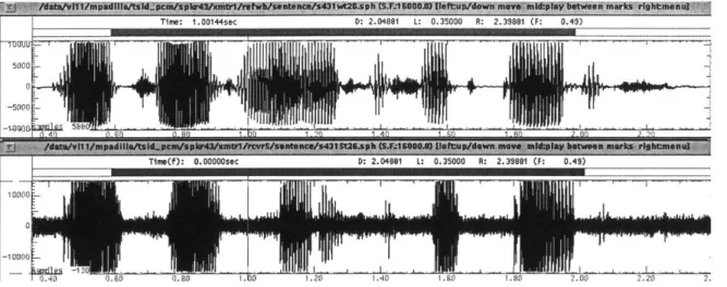
In this thesis, speaker verification within the setting of the TSID (Tactical Speaker ID) corpus, a collection of realistic recordings made of military personal at Ft. Bragg during spring 1997, is investigated. In total there were 35 speakers involved and recordings were made of soldiers reading sentences, digits, and map directions over a variety of very noisy and low bandwidth wireless radio channels. In this thesis these recordings are referred to as dirty speech files. For each dirty recording a low noise and high bandwidth reference recording was made simultaneously at the location of the transmitter with a microphone. These are referred to as clean speech files. In figures 1-5 and 1-6 are shown the time and frequency domain representations for the clean and dirty recordings of a representative utterance in the corpus. As may be seen from these plots, the waveform is subject to various types of nonlinear distortion as well as background ambient noise.
As would be expected given the discussion of the training/testing mismatch con-dition above, some verification tasks using both clean and dirty data for model train-ing and for testtrain-ing has shown that the clean/clean and dirty/dirty cases do
signif-V
Figure 1-5: Representative "clean" (top) and "dirty" (bottom) speech time-domain wave-forms from the TSID corpus. Both are from the same utterance.
rime: 0.9199 Freq: 0.00 Value: 67
!res =,,. 3
D: 2.03912 L: 0.35387 R: 2.39300 (F: 0.49)
Figure 1-6: Representative "clean" (top) and "dirty" (bottom) speech spectrograms from the TSID corpus. Both are from the same utterance.
ln
he I fndAA4 i - n iqnnn De -3 IQQQ4 IE. n AQ%
Baseline Case 80 -60 Io40 $20 - 0 *1
FaseAar poablTr(in las%)t it
5cnl
etri ro aepromneta Tra Dites Dimthcsso la/irty
20 ... ...
and dirty/clean, which have been found to perform nearly identically. These results are given in the DET curve in figure 1-7. It is seen that while the EER values for the clean/clean and dirty/dirty scenarios are approximately 4% and 9%, for the mis-matched cases it drops to nearly 50%. Note that since the decision being made is binary, an EER rate of 50% is equivalent to making a random guess for every test.
The focus of this thesis research is to study the effect of the mismatch condition on this database (training on clean and testing on dirty, or vice-versa) and to investigate ways of improving performance via the application of concepts in missing
feature
theory and spectral subtraction. missing feature theory recognizes the fact that due
to noise it is possible that some speech features could be corrupted to the degree that they no longer contain accessible speech information and that their inclusion in the statistical scoring mechanism could reduce performance. This requires the detection
of which features are missing and then their removal from scoring, done in such a way as to be consistent with the existing GMM model. This technique, known as missing feature compensation, is investigated along with the ability to accurately predict missing features. In addition, this thesis proposes a new manner to deal with the missing feature problem, time-frequency linear minimum mean-square error
(MMSE) feature estimation, in which the missing feature is detected, estimated, and then restored. This system is described along with some experimental results. Finally, a technique for subtracting out additive noise effects, known as spectral subtraction, is evaluated as is a new variation on this technique that is proposed in this thesis, to be termed soft
IDFT
spectral subtraction. In this thesis each of these techniques areexamined individually and in various combinations. In order to be able to control the evaluation and development of these techniques, throughout most of this thesis the clean TSID data files have been corrupted with known artificial additive noise. It is hoped that an understanding of the techniques explored in this thesis can be most readily achieved by first studying them in a controlled additive noise environment, making the transition later to unknown noise sources, such as the dirty TSID files, more feasible.
1.6
Contribution of Thesis
This thesis contributes to the body of knowledge in speaker recognition, specifically the train/test mismatch problem, in a number of ways. First, the performance of several established channel compensation techniques are applied to the clean/dirty verification problem in the context of the TSID database, thus extending our knowl-edge of how well these techniques can perform. Second, this thesis investigates the application of spectral subtraction in the
IDFT
domain, in contrast to the more common linear mel-filter energy domain, for the purpose of speech feature enhance-ment. It is demonstrated that the application of spectral subtraction in the |DFT domain is greatly superior for the type of additive noise channel being considered. Third, the application of missing feature theory, namely missing featurecompensa-tion, is studied and shown to improve performance over the baseline case for certain noise levels. In the process of this study, it is shown that the detection of missing features can be done non-ideally and still produce results highly correlated with an ideal detector. Forth, many of the channel compensation and missing feature meth-ods are combined to study recognition performance when these systems are applied in series. It is found that the combination of |DFT domain spectral subtraction and missing feature compensation performs very well, outperforming the baseline case and all other methods examined in this thesis. Finally, the concept of missing fea-ture estimation and restoration is explored. A linear minimum mean-squared error missing feature estimator, that operates in both the time and frequency domain, is derived and applied to both pure vowels as well as a TSID clean/dirty verification trial. While it does not improve performance in the verification trial, very promising results regarding the pre- and post-SNR levels for features estimated for the pure vowel indicate promise in the application of this approach.
1.7
Organization of Thesis
This chapter has introduced the general theory and problem of speaker verification, the statistical speaker model and speech features used, and the problem being ad-dressed within this framework along with some of the more important results within this thesis. In Chapter 2 various methods of channel compensation and a method for adding temporal information to the speech feature vectors are discussed along with results using these techniques on the TSID data in the mismatch scenario. Chapter
3 explains in detail the concepts of spectral subtraction and the proposed method of soft |DFT domain spectral subtraction, followed by a description of missing feature
theory and missing feature compensation in chapter 4. Both of these methods are evaluated using speech from the TSID corpus with a mismatch condition imposed through the addition of AWGN to the test data. Chapter 5 investigates what perfor-mance benefits are possible when the individual techniques in chapters 3 and 4 are combined in various combinations. The general method of missing feature
restora-tion, which tries to predict missing features rather than discard them as in missing feature compensation, is addressed in Chapter 6 along with the proposed technique of time-frequency linear MMSE missing feature estimation. These techniques are also evaluated with AWGN corrupted TSID speech. Finally, Chapter 7 summarizes the results presented in the thesis and suggests possible areas of future research.
Chapter
2
Channel Compensation and
Techniques for Robust Speaker
Recognition
The overall goal of speech feature selection in automatic speaker recognition is to ex-tract from a given speech waveform the most linguistically related signal components, while hopefully omitting unwanted elements such as noise and distortion imparted into the signal via both the channel and the speech apparatus itself. These degrada-tions may be additive, linearly convolutive, or nonlinear in nature and may contain modulation frequencies in part of or perhaps across the entire bandwidth of the speech signal. This is especially important in cases where speaker models are trained and tested in different environments, since leaving the channel characteristics in the train-ing speech will bias the speaker models in a way that will be uncompensated for in the testing speech. In essence, the speaker models will reflect not just characteristics of the speaker, but also those of the microphone, recording equipment, etc., result-ing in a mismatch condition brought about not by the underlyresult-ing speech, which is important, but rather by the environment in which the speech was recorded.
The following sections describe two methods for removing channel distortion from the speech features, cepstral mean subtraction and RASTA, as well as a method used to make the features somewhat more robust by including temporal feature
informa-tion. First the methods are described, followed by experimental results using these techniques in clean/dirty verification tasks.
2.1
Cepstral Mean Subtraction
Cepstral mean subtraction (CMS) attempts to remove from cepstral coefficient speech features convolutional distortion from a linear time-invariant channel[8]. Consider a scenario where a clean speech signal x[n] is passed through an LTI system h[n] producing a filtered output y[n]. Let this output y[n] be windowed by a time-limited function w[n] in order to extract segments of the signal for short time frequency analysis, producing the sequence yw [Min], where m denotes the short time segment and n denotes time
Yw Im, n] = (h[n] * x[n])w[m, n].
Given ywi[m, n], we would like to be able to recover x[n] without having to first estimate the system transfer function h[n]. This is known as blind deconvolution. Continuing from the above expression, if we assume that the nonzero duration of
w[m, n] is long and relatively constant over the duration of the channel response h[n],
then the following approximation may be made in the Fourier domain
F{yw[m, n]} = F{(h[n] * x[n])w[m, n]}
~ F{(x[n]w[m, n]) * h[n]}
=X[m, k]H[k]
which, for a fixed discrete frequency value k, is a time-trajectory in the parameter m. Applying the log operator then gives
log{Yw[m, k]} = log{X ,[m, k]H[k]}
= log{X,,[m, k]} + log{H[k]}.
m given by log{X,[m, k]} and a constant term given by log{H[k]}, representing the
channel. Since this channel term is a constant (DC), it may be removed by subtracting the mean value from each time-trajectory. Because typical speech has zero DC, this may be done without disturbing the speech term. This may be done by homomorphic liftering each of time-trajectories in the cepstral domain
c[m, k] = F-1 (log{X,[m, k]} + log{H[k]})
= x[m, k] + h[k]
- x^[m, k] + hk6[m].
Applying a cepstral lifter l[n] = 1 everywhere except for 0 at the origin will extract
2.2
RelAtive SpecTrA
2.2.1
Introduction and Basic System
Research has found that, much like the other sensory systems in the body, the auditory system tends to be sensitive to relative changes in an input signal, rather than absolute levels. Along these lines, there is evidence that the auditory system does not value signal components of all modulation frequencies equally [8]. Rather, there seems to be a peak in sensitivity to modulation frequencies around 4 Hz, with the relative sensitivity gradually decreasing as the frequency is decreased or increased. This modulation frequency of 4 Hz is sometimes referred to as the "syllabic rate". In addition, experiments conducted by van Vuuren and Hermansky[15] suggest that modulation frequencies below 0.1 Hz and above 16.0 Hz do not tend to be very relevant in determining the various speaker scores in automatic speaker recognition. These findings were further supported by Summerfield et al.[13] who showed that the perception of "speech-like" sounds depends strongly on the spectral difference between adjacent sounds, i.e. the temporal fluctuation of spectral components.
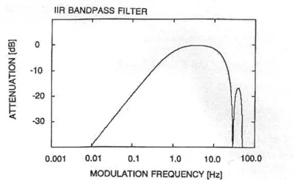
RelAtive SpecTrA (RASTA)[4] makes use of these findings by homomorphically filtering (liftering) the time-domain trajectories of the logarithmic cepstral speech features by an IIR bandpass filter with corner frequencies of about 0.26 Hz and 12.8 Hz and a peak at approximately 4 Hz (at the syllabic rate), with sharp notches at
28.9 Hz and 50 Hz. The transfer function for this filter is given by
0.Z2 + z- 1 - z-3 - 2z -4
H(z) = 0.1z
2
- - z1 - 0.98z 1
The high-pass denominator portion of this filter is to alleviate the convolutional noise introduced by the channel, while the low-pass portion is added to help smooth out the fast "instantaneous" spectral changes present in the short-term spectral estimates. The associated frequency and impulse responses are given in figures 2-1 and 2-2.
It is thus seen that RASTA suppresses speech feature components with modu-lation frequencies outside H(z)'s passband while keeping those seen as being most
IlR BANDPASS FILTER 0 -10 -20 -30 0.001 0.01 0.1 1.0 10.0 100.0 MODULATION FREQUENCY [Hz)
Figure 2-1: The frequency response of the RASTA filter H(w).
0.0
200.0
400.0
TIME [
rms]
relevant to automatic speaker recognition. Due to the spectral nulling at DC and other low frequencies below 0.26 Hz, we see that RASTA filtering will remove any time-invariant, similar to cepstral mean subtraction, as well as slowly time-varying linearly convolutive channel effects for each separate speech feature time-trajectory. The result is a reduction in the sensitivity of the new spectral feature estimate to slow and overly rapid variations in the short-term spectrum, brought about by static or slowly varying channels, noise, and unnecessary speech content.
2.2.2
Lin-Log RASTA
When performed as described above on cepstral features in the logarithmic domain, RASTA processing is most effective in diminishing the effects of time-invariant or slowly time-varying convolutional channel effects that are purely additive or nearly so (since an LTI channel will map to a linear additive term in the log spectral or cepstral domain). However, uncorrelated additive noise components that are additive in the log-magnitude domain, prior to the log operation, become signal dependent after the logarithmic operation is performed. To see this, consider in the frequency domain the output Y(w) of a linear system H(w) that is excited by a speech signal
S(w) and is corrupted by additive noise N(w):
Y(w) = H(w)S(w) + N(w)
log Y(w) = log [H(w)S(w) + N(w)]
= log {S(w)[H(w) + N(w)/S(w)]}
= log S(w) + log [H(w) + N(w)/S(w)]
It is observed that by the N(w)/S(w) term the noise is signal dependent and hence nonlinear, making RASTA processing by a fixed linear IIR filter as before not entirely appropriate for its removal from the speech signal.
uncorrelated additive noise, a family of alternative nonlinear transforms are employed instead of the standard logarithm. These nonlinear transforms have the property that they tend to be linear-like for small spectral values while log-like for large ones. The transform is parameterized by the single positive constant J and is given by
Y = log (1 + JX)
where X is the linear-domain speech feature and Y is the nonlinear transform of this feature. To gain some insight into the nature of this operation, it helps to rewrite the above expression slightly:
Y = log(1 + JX)
= log[J(1/J + X)]
= log(J) + log(1/J + X).
Upon the application of the RASTA filter h[n], the first term (a constant) is removed due to the high-pass portion of the filter. It is then seen that lin-log RASTA may be seen as a form of noise masking in which a fixed amount of additive noise is added prior to the RASTA processing in the logarithmic domain. This is somewhat similar to a technique employed in generalized spectral subtraction, which is described in chapter 3, in which additive noise is added to help mask musical tones[8].
To return to the linear domain, the following inverse is applied
X =y .
2.3
Delta Cepstral Coefficients
Delta cepstral coefficients (DCC) are used to impart temporal information into the
speech feature vector. In computing the coefficients, a low order polynomial is fit to to the features within a given window length over successive frames for each feature trajectory. The parameters of the derivative of the polynomial are used as an extra feature, appended to the end of the usual feature types discussed in section 1.3. In this sense, the use of this technique allows the speech features to contain information regarding the rate of change of formants and other spectral characteristics, possibly unique to a given speaker [12].
2.4
Results with TSID Corpus
To evaluate how well these techniques perform on real data, each of them was applied to the train clean/test dirty mismatch scenario with the TSID corpus. In this case, the actual narrowband noisy cellular data is used for the dirty test data. In all of the tests done in this section, the speech features used were cepstral coefficients and the sampling rate was 8 khz, resulting in 24 features. GMM speaker models were of order 1024.
As a means of comparison to what is possible in an ideal matched clean/clean case without any equalization applied (trials performed without any form of channel compensation of other noise management technique will hereafter be referred to as the baseline case), it was found that the corresponding EER was 4.2%. In contrast, it was found that the baseline mismatch case of train clean/test dirty 1 had an EER of approximately 50%, signifying that in the baseline mismatch case for the TSID data the system is essentially flipping a coin to make its accept/reject decisions.
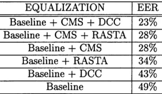
In applying the techniques of CMS, RASTA, and DCC, both individually and in combination, the results in table 2.4 were found.
EQUALIZATION
EER
Baseline + CMS + DCC 23% Baseline + CMS + RASTA 28% Baseline + CMS 28% Baseline + RASTA 34% Baseline + DCC 43% Baseline 49%Table 2.1: Results applying various channel compensation techniques to TSID data for train clean/test dirty case.
The corresponding DET curve is given in figure 2-3.
'Results throughout this research have shown that the performance in many cases of the train clean/test dirty case is nearly identical to that of the train dirty/test clean case. Due to this observation and the fact that the most likely scenario is clean data during training and dirty data during testing, this thesis focuses on the train clean/test dirty case.
80 . .. ... ... . .. -- Base -4* Base+CMS Base + RASTA -- - Base + CMS+ RASTA - Bas + DCC -Bs+DCC+CMS 60 - -- - -- + - --- Base - - .--+--- . -SBase C Base + RASTA
I oapis note are tCaSt .aslneRASTA CM a.se prdcda
0 U) I as~kw~cc + CI~S 20 .. .. .. . ... .. . . . .. . . .. .N . . . . . .. . .. . . . . . . 10 10 20 4 08
False Alarm probability (in %)
Figure 2-3: Comparison of various equalization techniques.
Important points to note are that the Baseline + RASTA + CMS case produced an EER of 28%, which is the same as the Baseline + CMS case, without RASTA being applied. As discussed in the introductory part of this chapter, RASTA has been developed for the purpose of removing slowly varying convolutional distortion, hence its removal of small quefrencies2 from 0 to 0.1 Hz. CMS, on the other hand, is only able to remove strictly time-invariant convolutional distortion through the liftering out of the 0th cepstral coefficient for each temporal trajectory. The fact that the EER values for the systems of CMS + RASTA and CMS alone perform the same at 28% indicates that for the TSID corpus that the most corruptive convolutional distortion is likely to be of a time-invariant nature, hence the lack of additional improvement from RASTA when CMS is already applied. It is also observed that DCC alone does not help performance very much, while adding DCC on top of CMS improves performance slightly from 28% to 23%, producing the best performing system that
2Frequency in the cepstral domain is frequently referred to as "quefrency", noting the reversed
role played by time and frequency in this domain. This also explains the the motivation for the terminology "cepstral" (spectral) and "liftering" (filtering).
Chapter 3
Spectral Subtraction
This chapter investigates a general methodology to deal with the corruption of speech features with additive noise. It is a well established and intuitively reasonable fact that as speech is degraded by ambient background noise that the resulting automatic speaker recognition performance decreases dramatically. One approach to alleviating this effect is to devise speech features that are sufficiently robust to the noise types and levels so as to make estimation of the noise characteristics unnecessary. The approach discussed in this chapter, spectral subtraction (SS), makes the assumption that the type and level of noise affecting the speech is amenable to being effectively estimated attempts to derive a spectral characterization of the additive noise process effecting the speech such that it may be subtracted from the spectral magnitude of the corrupted speech waveform. While this operation is typically done in the IDFT
domain, applications in the speech recognition and verification for the purpose of cleaning up speech features have focused on performing the spectral subtraction in the linear Mel-filter energy domain. This thesis proposes that it be done one stage earlier in the calculation of the speech features at the |DFT stage prior to the application of the Mel-filters. This provides a "softer" form of spectral subtraction that will be shown to be superior to traditional spectral subtraction. This chapter concludes by reporting several results obtained when these techniques were applied to the TSID corpus in a clean/dirty mismatch scenario, the dirty data being a result of additive white Gaussian noise.
3.1
Mel-Filter Energy Domain Spectral
Subtrac-tion
First we will consider the spectral subtraction in the domain in which is has typically been applied when the goal is to enhance speech features, in the linear mel-filter energy domain.
Consider a speech signal x[n] that has been corrupted by additive stationary ambient noise a[n], producing a noisy speech signal y[n]
y[n] = x[n] + a[n],
the spectral magnitude of which is
|Y(w)|2 =
IX(w)
+ A(w)|2= [X(w) + A(w)]*[X(w) + A(w)]
= IX(w)12 +
IA(w)1
2+ X*(w)A(w) + X(w)A*(w).
If we make the reasonable assumption that x[n] and a[n] are uncorrelated wide-sense stationary (WSS) processes, then taking expectations gives us
E[|Y(w) 12] =
E[IX(w)1
2+IA(w)1
2 + X*(w)A(w) + X(w)A*(w)]= E[IX(w) 12] + E[IA(w) 12] + E[X*(w)A(w)] + E[X(w)A*(w)]
= E[IX(w) 12] + E[|A(w) 12] + E[X*(w)]E[A(w)] + E[X(w)]E[A*(w)]
= E[IX(w) 12] + E[IA(w) 12]
since the complex spectra of both the speech and the ambient noise will typically be zero mean. If the spectral magnitude IY(w)|2 is then input to the mel-filterbank, composed of filters M[k], then on the average the resulting linear mel-filter energy