An application of robust H₂/H[infinity] control synthesis to launch vehicle ascent by Tyler Nicklaus Hague.

(1)

An Application of Robust H

2

/H,. Control Synthesis to

Launch Vehicle Ascent

by

Tyler Nicklaus Hague

B.S. Astronautical Engineering United States Air Force Academy, 1998

SUBMITTED TO THE DEPARTMENT OF AERONAUTICS AND

ASTRONAUTICS IN PARTIAL FULFILLMENT OF THE REQUIREMENTS FOR THE DEGREE OF

MASTER OF SCIENCE

at the

MASSACHUSETTS INSTITUTE OF TECHNOLOGY

June 2000

The author hereby grants to MIT permission to reproduce and to distribute publicly paper and electronic copies of this thesis document in whole or in part.

Signature of Author:

D armeht Ae'ron'auti ", stroqautics

Certified by:

Fr 1erick W. NoeIitz Charles Stark Draper Laboratory Technical Supervisor Certified by:

Profedsor John J. Deyst Professor of Aeronautics and Astronautics Thepis Advisoy Accepted by:

Nesbitt W. Hagood III

MASSACHUSETTS INSTITUTE Professor of Aeronautics and Astronautics OF TECHNOLOGY Chairman, Department Graduate Committee

(2)

MITLibraries

Document Services Room 14-0551 77 Massachusetts Avenue Cambridge, MA 02139 Ph: 617.253.2800 Email: docs@mit.edu http://Iibraries.mit.edu/docs

DISCLAIMER OF QUALITY

Due to the condition of the original material, there are unavoidable flaws in this reproduction. We have made every effort possible to

provide you with the best copy available. If you are dissatisfied with this product and find it unusable, please contact Document Services as

soon as possible.

Thank you.

The images contained in this document are of

the best quality available.

(3)

An Application of H

2

/H. Robust Control Synthesis to Launch

Vehicle Ascent

by

Tyler Nicklaus Hague

Submitted to the Department of Aeronautics and Astronautics on May 5, 2000 in Partial Fulfillment of the Requirements for the Degree of Master of Science in Aeronautics and Astronautics

ABSTRACT

This thesis explores the application of H2/H. control synthesis methods to

launch vehicle ascent, specifically the pitch-plane control of the Kistler Aerospace launch vehicle, K1. A classical single-input, single-output design is also

presented in order to assess the true applicability of a modern control synthesis approach to launch vehicle ascent. In addition, the K1 dynamics are developed to include aerodynamic, fuel-sloshing, tail-wags-dog, and body-bending effects. The objective of the modern control synthesis approach presented here is to design compensation for pitch tracking and disturbance rejection. It combines techniques in optimal H2, optimal H., and sub-optimal control synthesis to create

pitch control laws that provide 6 dB of gain margin and 302 of phase margin. The sensitivity and high-order of traditional H2/H. synthesis are addressed through

the implementation of uncertainty in the design model and the application of balanced, model order reduction on the resulting controllers. To reduce the complexity in applying these methods, a hierarchical approach and design strategy is employed. Additionally, a graphical user interface is presented that exploits the capabilities of commercial software during the design.

A comparison of the two design methods, classical and modern, reveals

that each design architecture is capable of creating controllers of equivalent order with both nominal and robust performance. The advantages of the modern approach are realized in the design process itself. The hierarchical methodology and intuitive nature of the modern approach helps to manage the selection of design parameters. Whereas, classical methods provide less insight into

strategies for parameter selection and control design. Additionally, the ability to address disturbances and uncertainty in the modern approach offers a more direct alternative to the ad hoc and iterative nature of classical methods, and although not fully exploited here, the modern approach does allow coupling between channels to be accommodated. These conclusions confirm the viability of a modern control synthesis approach and establish the foundation for future development of modern-based, ascent control laws.

(4)

Thesis Supervisor: Frederick W. Boelitz

Title: Senior Member of the Technical Staff, Charles Stark Draper Laboratory

Thesis Advisor: Professor John J. Deyst

(5)

ACKNOWLEDGEMENTS

I would like to express my sincere gratitude to a number of people.

Without their support, this thesis would not have been possible.

First, I would like to thank Fred Boelitz. His expertise in control design and familiarity with the Kistler control problem were an invaluable source of information and guidance. But, most importantly, I always felt that as my

supervisor he cared more about my personal development and made sure I grew throughout the thesis experience. It has been a pleasure to work for him.

I also thank Dr. Brent Appleby, Professor John Deyst, and Mrs. Bette

James for their contributions to the development of this thesis. Each provided invaluable comments and direction. A special thanks to Mrs. James for offering her talents and making sure that the ideas put into thesis were able to make it out.

I would also like to thank all of my MIT/Harvard friends, especially Scott,

George, Jim, Troy, and Chris. Thanks for making my time in Boston a

memorable one. I would like to give additional thanks to Scott for putting up with me every hour of every day for the last 4 years. He has been a valued friend, and his influence on my work is undeniable.

I want to thank my family for love and support they have given throughout

my life. I have always been able to count on them. Thanks.

Finally, I want to thank Catie. Her friendship and love have brought out the best in me, and made me realize what I can accomplish. Thank you for being my constant source of inspiration.

This thesis was prepared at the Charles Stark Draper Laboratory, Inc. under Individual Research and Development funding, Project 15118. Publication of this thesis does not constitute approval by Draper or the sponsoring agency of the findings or conclusions contained herein. It is published for the exchange and stimulation of ideas.

(6)

(7)

List of Figures

Figure 1.1 - Indirect Adaptive Control Loop Structure 23

Figure 1.2 - Dynamic Inversion Framework ... 25

Figure 2.1 - Boost Phase Propulsion System Components ... 32

Figure 2.2 - K1 TVC Physical Description ... 33

Figure 2.3 - Representative TVC Loop ... 34

Figure 2.4 - Body Axis System... 35

Figure 2.5 - Pitch Plane Free-Body Diagram ... 36

Figure 2.6 - Nominal Trajectory Dynamic Pressure Profile ... 42

Figure 2.7 - Nominal Trajectory Mach Profile... 43

Figure 2.8 - Design Model Nichols Chart ... 45

Figure 2.9 - Design Model Bode Plot ... 46

Figure 3.1 - Classical Canonical Form. ... 50

Figure 3.2 - CSDL SISO Control Loop Realization. ... 50

Figure 3.3 - Modified PD Open Loop Frequency Response...55

Figure 3.4 - Modified PD Nichols Plot ... 56

Figure 3.5 - SISO Design Step Responses... 63

Figure 3.6 - SISO Design Frequency Responses ... 63

Figure 4.1 - H2/H. Control Design Loop... 66

Figure 4.2 - Reference Input in MIMO Control Loop ... 71

Figure 4.3 - Wind Input in MIMO Control Loop... 72

Figure 4.4 - NASA Wind Gust Model ... 73

Figure 4.5 - Noise Inputs in MIMO Control Loop... 74

Figure 4.6 - "False" Inputs in MIMO Control Loop... 75

(14)

Figure 4.8 - U(s) Penalty Shaping Filter... 76

Figure 4.9 - Sensitivity Cost Output in MIMO Control Loop... 77

Figure 4.10 - General Control Loop Structure ... 78

Figure 4.11 - Sensitivity Waterbed Effect ... 79

Figure 4.12 - S(s) Penalty Shaping Filter ... 80

Figure 4.13 - Control Inputs Input in MIMO Control Loop ... 81

Figure 4.14 - Control Output in MIMO Control Loop ... 82

Figure 4.15 - Nominal Loop Configuration ... 85

Figure 4.16 - Gain Augmentation ... 86

Figure 4.17 - Multiplicative Uncertainty ... 87

Figure 4.18 - Multiplicative Uncertainty Implementation...88

Figure 4.19 - Fit Analysis of Uncertainty Weight ... 89

Figure 5.1 - Control Synthesis Hierarchy ... 100

Figure 5.2 -- H2/H. Solution Process ... 102

Figure 5.3 - Robust Control Synthesis GUI ... 105

Figure 5.4 - Multiplicative Uncertainty Design Model ... 108

Figure 5.5 - Gain Augmentation Design Model ... 109

Figure 5.6 - Initial Weights for Cost Outputs, Zs(s) and zu(s)...111

Figure 5.7 - Pole-Zero Map of Full-Order, Optimal H2 Controller ... 112

Figure 5.8 - Final Weights for Cost Outputs, zs(s) and zu(s)...114

Figure 5.9 - Maximum Singular Values for the Optimal H2, Optimal H., and Sub-O ptim a l D e sig ns ... 1 16 Figure 5.10 - Initial Full-Order H2 Design Step Response...118

Figure 5.11 - Initial Full-Order H2 Design Frequency Response ... 118

Figure 5.12 - Improved Full-Order H2 Design Step Response ... 119

Figure 5.13 - Improved Full-Order H2 Design Frequency Response...119

Figure 5.14 - Optimal Full-Order H2 Design Step Response...120

Figure 5.15 - Optimal Full-Order H2 Design Frequency Response ... 120

Figure 5.16 - Optimal Full-Order H. Design Step Response ... 121

Figure 5.17 - Optimal Full-Order H. Design Frequency Response...121

(15)

Sub-Optimal Full-Order Design Frequency Response...122

Figure 5.20 - K1 Plant Com parison...124

Figure 5.21 - G=1.0, GA H2 Design Step Response ... 129

Figure 5.22 - G=1.0, GA H2 Design Frequency Response...129

Figure 5.23 - G=2.0, GA H2 Design Step Response ... 130

Figure 5.24 - G=2.0, GA H2 Design Frequency Response...130

Figure 5.25 - GA H. Design Step Response...131

Figure 5.26 - GA H,, Design Frequency Response ... 131

Figure 5.27 - GA Sub-Optimal Design Step Response ... 132

Figure 5.28 - GA Sub-Optimal Design Frequency Response...132

Figure 5.29 - Step Response Comparison ... 133

Figure 5.30 - Frequency Response Comparison ... 134

Figure 5.31 - GA=1 .0, MU H2 Design Step Response ... 139

Figure 5.32 - GA=1.0, MU H2 Design Frequency Response...139

Figure 5.33 - GA=10, MU H2 Design Step Response ... 140

Figure 5.34 - GA=10, MU H2 Design Frequency Response...140

Figure 5.35 - GA=20, MU H2 Design Step Response ... 141

Figure 5.36 - GA=20, MU H2 Design Frequency Response...141

Figure 5.37 - MU Hc. Design Step Response ... 142

Figure 5.38 - MU H. Design Frequency Response...142

Figure 5.39 - MU Sub-Optimal Design Step Response...143

Figure 5.40 - MU Sub-Optimal Design Frequency Response ... 143

Figure 5.41 - Controller O rder Com parison...145

Figure 5.42 - Reduced-Order, GA Robust H2 Design Step Response...150

Figure 5.43 - Reduced-Order, GA Robust H2 Design Frequency Response.... 150

Figure 5.44 - Reduced-Order, MU Robust H2 Design Step Response...151

Figure 5.45 - Reduced-Order, MU Robust H2 Design Frequency Response ... 151

Figure 5.46 - Modified Control Loop Architecture...154

Figure 5.47 - Step Response of 7th and ₈th Order Controllers...157

Figure 5.48 - Frequency Response of 7th and ₈th Order Controllers ... 158 Figure 5.19

(16)

-Figure 5.49 - Step Response of 10th and 12th Order Controllers ... 159

Figure 5.50 - Frequency Response of 10th and 12th Order Controllers ... 159

Figure 6.1 - Step Response Comparison ... 165

Figure 6.2 - Nichols Frequency Response Comparison...166

Figure 6.3 - Bode Frequency Response Comparison ... 166

Figure 6.4 - Wind Response Maximum Singular Value...169

Figure 6.5 - Angular Position Noise Response Maximum Singular Value...169

Figure 6.6 - Angular Rate Noise Response Maximum Singular Value...170

Figure 6.7 - Simulated Reference Input ... 172

Figure 6.8 - Simulated Wind Gust Input ... 172

Figure 6.9 - Comparison of Simulated Pitch and Gimbal Responses ... 173

Figure A.1 - General body with rotation about CG ... 187

Figure A.2 - Gravity Free-Body Diagram...193

Figure A.3 - Thrust Free-Body Diagram...194

Figure A.4 - TWD Free-Body Diagram...196

Figure A.5 - Angle of Attack Definition ... 201

Figure A.6 - Slosh Free-Body Diagram ... 203

Figure A.7 - IMU Reference Diagram...207

Figure A.8 - Body Bending Effects on Engine Gimbal...212

Figure B.1 -- Steady-State Pitch Angle Profile ... 221

Figure B.2 - Steady-State Angle of Attack Profile ... 222

Figure B.3 - Steady-State Center of Gravity Location Profile...222

Figure B.4 - Steady-State Acceleration Profile ... 223

Figure C.1 - Rigid Body Response Comparison ... 226

Figure C.2 - Simple Aerodynamic Response Comparison ... 227

Figure C.3 - Simple Aerodynamic Model Comparison ... 228

Figure C.4 - Complex Aerodynamic Response Comparison...230

Figure C.5 - Complex Aerodynamic Model Comparison ... 231

Figure C.6 - Small Angle Approximation Region of Validity ... 232

Figure C.7 - Comparison of Tail-Wags-Dog Zero Histories...233

(17)

Figure C .9 - R P Slosh Frequency ... 235

Figure C .10 - RP Dam ping Coefficient...235

Figure C.11 - RP Slosh Mode Pole/Zero History...236

Figure C.12 - LOX Slosh Frequencies ... 237

Figure C.13 - LOX Dam ping Coefficients...237

Figure C.14 - LOX Main Slosh Mode Pole/Zero History...238

Figure C.15 - LOX Retention Mode Pole/Zero History ... 239

Figure C.16 - Flex Mode Pole/Zero Pairs at Mach 1.0 ... 240

Figure D.1 - SISO Loop Transfer Function SIMULINK Model...245

Figure D.2 - SISO Closed Loop Transfer Function SIMULINK Model...245

Figure E.1 - Actuator Uncertainty Representations...249

Figure F.1 - Full-Order Optimal H2 Design 3-c Step Response History ... 268

Figure F.2 - Full-Order Optimal H2 Design 3-a Nichols Plot History...268

Figure F.3 - GA Optimal H2 Design 3-i Step Response History ... 269

Figure F.4 - GA Optimal H2 Design 3-c Nichols Plot History...269

Figure F.5 - GA Optimal H2 Design 1-c Step Response History ... 270

Figure F.6 - GA Optimal H2 Design 1-cy Nichols Plot History...270

Figure F.7 - GA Sub-Optimal Design 3-c Step Response History ... 271

Figure F.8 - GA Sub-Optimal Design 3-c Nichols Plot History ... 271

Figure F.9 - GA Sub-Optimal Design 1-c Step Response History ... 272

Figure F.10 - GA Sub-Optimal Design 1-c Nichols Plot History ... 272

Figure F.1 1 - GA=1, MU Optimal H2 Design 3-G Step Response History ... 273

Figure F.12 - GA=1, MU Optimal H2 Design 3-y Nichols Plot History ... 273

Figure F.13 - GA=10, MU Optimal H2 Design 3-cy Step Response History ... 274

Figure F.14 - GA=10, MU Optimal H2 Design 3-a Nichols Plot History ... 274

Figure F.15 - GA=20, MU Optimal H2 Design 3-cy Step Response History ... 275

Figure F.16 - GA=20, MU Optimal H2 Design 3-G Nichols Plot History ... 275

Figure F.17 - GA=20, MU Optimal H2 Design 1-G Step Response History ... 276

Figure F.18 - GA=20, MU Optimal H2 Design 1-cT Nichols Plot History...276

(18)

Figure F.20 - MU Sub-Optimal Design 3-cy Nichols Plot History...277 Figure F.21 - Reduced-Order GA Optimal H2 Design 3-cy Step Response History

... ... 2 7 8

Figure F.22 - Reduced-Order GA Optimal H2 Design 3-(T Nichols Plot History 278

Figure F.23 - Reduced-Order GA Optimal H2 Design 1 -(T Step Response History

... 2 7 9

Figure F.24 - Reduced-Order GA Optimal H2 Design 1 -(T Nichols Plot History 279

Figure F.25 - Reduced-Order MU Optimal H2 Design 3-cy Step Response History

... 2 8 0

Figure F.26 - Reduced-Order MU Optimal H2 Design 3-a Nichols Plot History281

Figure F.27 - Reduced-Order MU Optimal H2 Design 1-cy Step Response History

... 2 8 1

(19)

List of Tables

Table 2.1 - LAP Design Model Parameters...44

Table 2.2 - Mode Shape Parameters for first 10 Bending Modes ... 44

Table 3.1 - Dispersion Parameter Summary...53

Table 3.2 - Classical Design Parameters... 58

Table 3.3 - Successful SISO Design Results ... 59

Table 3.4 - Relaxed Attenuation Results...60

Table 3.5 - Design Alpha Dispersion Results... 61

Table 3.6 -- Design Beta Dispersion Results ... 61

Table 5.1 - Full-Order Design Phase Summary ... 117

Table 5.2 - G=1.0, GA H2 Design Performance Metrics...125

Table 5.3 - G=2, GA H2 Design Performance Metrics...126

Table 5.4 - GA H. Design Performance Metrics ... 127

Table 5.5 -- GA Sub-Optimal Design Performance Metrics ... 127

Table 5.6 - GA Robust Design Summary...128

Table 5.7 - GA=1.0, MU H2 Design Performance Metrics...135

Table 5.8 - GA=10, MU H2 Design Performance Metrics ... 135

Table 5.9 - GA=20, MU H2 Design Performance Metrics...136

Table 5.10 - MU H. Design Performance Metrics ... 137

Table 5.11 - MU Sub-Optimal Design Performance Metrics ... 137

Table 5.12 - MU Robust Design Summary...138

Table 5.13 - GA Robust H2 Design HSVs ... 144

Table 5.14 - GA Robust H2 Design Order Reduction Summary...145

(20)

Table 5.16 - MU Robust H2 Design Order Reduction Summary ... 146

Table 5.17 - Reduced-Order Design Summary...147

Table 5.18 - Final Control Design Summary ... 160

Table 5.19 - MCS Summary...161

Table 6.1 - Performance Metric Summary ... 164

Table 6.2 - Figure Legend ... 165

Table 6.3 - Actuator Perturbation Results ... 174

Table E.1 - Individual 3-Y Test Cases...247

Table E.2 - Combined 1-a Test Cases...250

Table E.3 - Design Alpha 3-y Results ... 251

Table E.4 - Design Alpha - 1 -c Results ... 253

Table E.5 - Design Beta - 3-y Results...255

Table E.6 - Design Beta - 1 -T Results...257

Table E.7 - Design Gamma - 3-Y Results ... 258

Table E.8 - Design Gamma - 1 -Y Results ... 261

Table E.9 - Design Delta - 3-y Results...262

(21)

CHAPTER 1 Introduction

The objective of this thesis is to present a viable alternative to the classical control synthesis method currently used to design the ascent control law for the Kistler Aerospace launch vehicle, K1. Based on concepts from multivariable control systems theory, this thesis explores an alternative approach for a specified design point in the boost phase trajectory. A comparative analysis is presented, using a control law derived from classical principles, which highlights the capabilities and limitations of the Modern Control Synthesis (MCS) approach considered in this thesis. In conjunction with the modern control law

development, an advanced set of linearized equations of motion (EOMs) are presented for the K1. These EOMs include rigid body motion, aerodynamic lift and drag, fuel-sloshing, engine inertia, and body-bending effects.

1.1 Problem Motivation

Classical, or Single-Input Single-Output (SISO), design techniques have been used extensively throughout the history of the launch vehicle industry, and the familiarity and success of these methods have helped to sustain their use in many in current applications. However, the SISO design process can be less intuitive, than more modern methods and usually requires numerous iterations and refinements. Furthermore, classical design techniques lack the ability to handle system disturbances and modeling errors simultaneously during the design process. Accounting for these multiple, naturally occurring factors can

(22)

quickly become an overwhelming task for the designer of a classical control system.

The maturity of modern control theory and the availability of software that supports Multiple-Input Multiple-Output (MIMO) applications now make MCS synthesis a viable alternative to classical methods. Both classical and modern methods are capable of designing successful controllers, but MCS design methods address the shortcomings of SISO synthesis. Problem formulation using MCS is intuitive and incorporates system disturbances, sensor noises, and model uncertainties: allowing it to account for multiple, coupled channels.

Additionally, MCS synthesis generates controllers in a more direct manner through the solution of two Riccati equations.

1.2 General Problem Statement

Due to the shortcomings of classical design methods, there is a need to develop a more direct and intuitive approach for designing a first-stage, K1 control law. Not only are the requirements of nominal and robust performance significant, but the design process itself is also of importance. The primary goal of this thesis is to present a practical application of a systematic design

methodology that can address many of the typical design challenges encountered with launch vehicles.

1.3 Approach

In order to select a proper basis for an alternative design method, initial research assessed several new areas of control synthesis for their applicability to launch vehicle boost phase control. This research explored two main control areas with an extensive background and a history of application at The Charles

Stark Draper Laboratory: adaptive control and gain-scheduled linear control. Within adaptive control, Model Referencing Adaptive Control (MRAC) and

Dynamic Inversion (DI) were studied. Within gain-scheduled linear control, which is the traditional ascent control law implementation, several control synthesis

(23)

techniques were also explored for ascent control application. Convex

optimization, robust weighted H2/H,. control, and ji-synthesis are all maturing

techniques that have previously been applied to other "real-world" problems.

By successfully applying one of these possible modern control

methodologies, or combining techniques from several approaches, an alternative first-stage control law can be developed. And, by comparison with a benchmark classical controller, the modern design methodology can be assessed for its applicability to K1 ascent.

1.3.1 Model Referencing Adaptive Control (MRAC)

MRAC is a form of direct adaptive control in which the controller monitors its own performance and adjusts one or more control parameters to achieve a desired response. The application of MRAC to launch vehicle control was

studied by both Whitaker [30] and Best [4] since the 1960s. The drawback to this approach is the difficulty of maintaining stability in the presence of unmodeled dynamics, system disturbances, and sensor noise [2].

Variants of the direct adaptive approach have also been investigated. So-called, indirect adaptive control methods have recently been applied to, among other things, autonomous underwater vehicles by Claudberg [9]. Figure 1.1 shows a control loop representation of the indirect adaptive control approach.

Parameter Estim ate

State Estimate dysemiiat

Reference _Output

Input Contro IF U Plant

Figure 1.1 - Indirect Adaptive Control Loop Structure

This method, aided by computer technology, uses system identification techniques to overcome the problems associated with the unmodeled error

(24)

encountered by Whitaker and Best. By accessing the plant inputs and outputs, a model of the physical plant is generated using system identification techniques, which the controller uses for system state and control parameter estimates.

However, this techniques requires extensive on-line computational power and is too complex an alternative for application to the K1.

1.3.2 Dynamic Inversion

The Dynamic Inversion (DI) design methodology, or feedback

linearization, has been studied by Bedrossian [2], and extensively explored for its application to the micro air vehicle (MAV) by Brown [8], and the F-1 8 High Angle-of-Attack Research Vehicle (HARV) by Reigelsperger, et. al. [27]. With DI the controller comprises two elements (Figure 1.2). The first is a model of the desired plant dynamics, and the second is a dynamic inverter. The dynamic inverter effectively cancels the system dynamics using state and output measurements. Once the plant dynamics are inverted, the desired response shapes the closed-loop transfer function. An obvious limitation to this approach is the requirement of full state information [2]. Within the current K1 control framework, the fuel-sloshing and bending states are not measured, and the zero dynamics of the system become critical to stability [28]. To overcome a similar problem in large flexible aircraft, extra sensors were added to airframe

extremities to sense the wing flex states [14]. Additionally, exact inversion of the plant dynamics make this control technique extremely susceptible to errors in the plant model. Considering the inability to sense slosh and bending states on the K1 and the need for an extremely accurate plant model, DI will not be considered as an alternative approach.

(25)

Controller

Input Otu

Desired Dyn cPlant

Response Invert

Figure 1.2 - Dynamic Inversion Framework

1.3.3 Constrained Convex Optimization

Constrained convex optimization is another synthesis method that has received much attention. Advanced by the increased capability of linear program solvers, constrained convex optimization has been applied to the Draper Small Autonomous Aerial Vehicle (DSAAV), the Earth Observing System (EOS)

spacecraft, and the Active Vibration Isolation System (AVIS) in [20, 17]. Offering an alternative to both classical and model-based approaches, this method utilizes Youla (or Q) parameterization to obtain a solution from a predetermined set of basis functions. The central difficulty arises from the proper selection of basis functions, which increases the complexity of the synthesis process. In order to mature this ad hoc selection process, further research into a general set of orthonormal basis functions will be required [17].

1.3.4 p Synthesis

g-Synthesis is one of the more powerful synthesis tools available today, and has also been applied to the F-18 HARV [27]. An extension of the optimal H. approach discussed in Chapter 4, g-Synthesis uses structured uncertainties to achieve guaranteed robustness and specified performance levels. Composed of multiple complex techniques, g-analysis, D-scaling, and H. minimization, the design process has proven to be computationally intensive [15]. Furthermore, downfalls of this approach are the size of controllers it generates and its over-conservative guarantees for robustness, which lead to reduced performance capability [15].

(26)

1.3.5 Robust Weighted H2/H. Based Designs

Optimal H2/H. design methods are fundamental concepts in MCS theory.

H2/H. refer to the norms of the cost function minimized during the design

process. For an H2 design, the norm is the average singular value; for an H.

design, it is the peak singular value. Alone, these model-based approaches are not particularly interesting, offering no advance to traditional loop shaping

techniques [27]. Because they contain state estimates of the models for which they are designed, H2/H. designs are very sensitive to modeling errors and are

high in order. However, augmenting these fundamental design methods with frequency cost-weights and system uncertainties, and applying model order

reduction techniques can achieve successful results [15]. Implementing this approach can produce a synthesis process that is simple and intuitive with direct physical meaning. Not without its own drawbacks, a robust weighted H2/H.

approach can still produce higher order controllers, and problem formulation can sometimes be difficult. However, this approach appears to be the most viable alternative to the current classical methods used in the K1 design and will serve as the foundation for the development of an MCS framework.

1.4 Scope

A central goal of this thesis is the successful demonstration of the

alternative design process's applicability. To this end, great effort was taken to limit the simplifications and assumptions used in the multivariable framework. However, several notable simplifications and assumptions were deemed necessary and appropriate to aid in the completion of this work. These simplifications and assumptions will be discussed at length in the following sections.

1.4.1 Continuous Time Solution

Although the physical system is best described with continuous non-linear, time varying differential equations, the math models utilized in the design

(27)

framework are simplified to continuous linear time invariant (LTI) systems that characterize only the dynamics associated with small perturbations from equilibrium. This linearization process is fundamental to the gain-scheduled linear control synthesis technique, in which many point designs are made along the trajectory and blended together. However, the physical implementation of the final ascent control law is digital. For this thesis, the design process has been restricted to continuous analysis. Studies surrounding the continuous-to-digital conversion of the controllers and its impact on system performance are left for future research.

1.4.2 Boost Phase Pitch Plane Control

The development of a control synthesis methodology for K1 ascent is limited to the pitch plane only, which is defined in Chapter 2. This limitation assumes that the symmetry of the K1 permits the extension of any pitch plane analysis into the lateral plane. Therefore, the lateral and longitudinal motions will

be uncoupled using reasonable assumptions consistent with past experience. Roll and yaw control are viewed as a separate, decoupled problem and are not considered in this work.

1.4.3 Design Point Selection

By choosing times during the boost phase for which control design has

traditionally been difficult, the extension of the modern synthesis framework to other design points is assumed to be a relatively easy task. Traditionally, the most difficult design points during a boost phase trajectory are the transonic region (Mach 1.0) and the time at which maximum dynamic pressure, Q, occurs. For the K1, these two points occur within seconds of each other, approximately

72 seconds after launch. Therefore, only one point (Mach 1.0, Q = 480 psf)

during the mission trajectory will be used as a basis for the comparison of the classical and multivariable synthesis methods. In developing the modern control synthesis method for this dynamically severe point in the trajectory, it is assumed that the design method can be extended with less challenge to further design

(28)

points in order to develop a control law for the entire boost phase. Obviously there will be issues surrounding the blending of controllers for the various point designs, but those issues are common to all gain-scheduled linear control approaches, both modern and classical, and are not investigated here.

1.4.4 Design Method Portability

Although the Kistler flight control problem has several unique aspects, many of the issues that must be addressed in its design are common to a larger, more general class of launch vehicles. Dynamic effects associated with forces caused by flexure, slosh, aerodynamics, engine motion, and actuators are topics central to a majority of launch vehicle control law designs; these effects are considered for the Kistler launch vehicle. The research presented here is intended to provide a viable engineering example from which concepts can be extracted and applied to a large class of launch vehicle control problems.

1.5 Thesis Preview

Following the introductory chapter, this thesis is organized as follows.

Chapter 2 presents the K1 physical system description and its associated reference frames. The development of the K1 pitch plane linearized EOMs is also presented along with discussion of the frequency response contributions of each dynamic effect. Inertial measurement unit (IMU) and actuator dynamics are briefly discussed, as well as associated computational delays.

Chapter 3 summarizes the classical design approach used to develop a pitch plane controller for the Mach 1.0 point. A brief summary of the existing Proportional-Derivative boost phase controller is presented to establish the need for a forward path bending filter. A gain vector search algorithm is used to

automate the design process, and successful resulting controllers are analyzed.

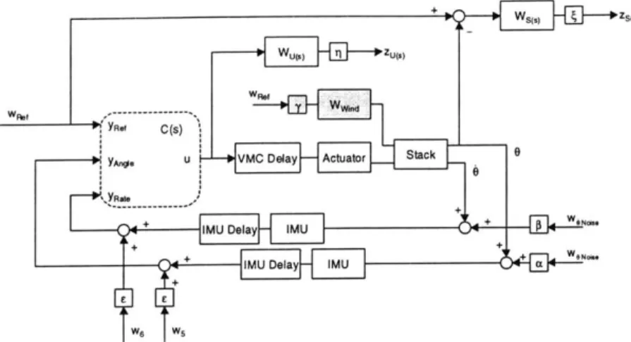
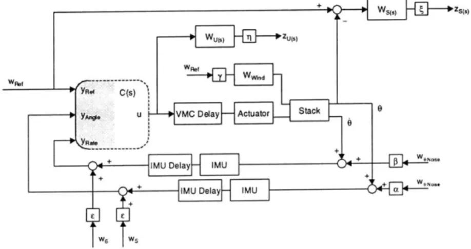
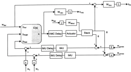
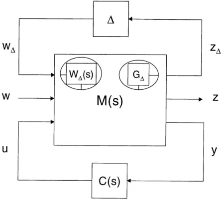
Chapter 4 contains the background necessary to understand the modern control framework created to design robust H2/H. controllers. The canonical

(29)

problem formulation is discussed along with controllability and observability issues. Insight into weighting function selection is also provided. Finally,

concepts surrounding the implementation of uncertainty in control law design, as well as controller order reduction, are addressed.

Chapter 5 presents the implementation of the framework addressed in Chapter 4. The MATLAB graphical user interface (GUI) and its supporting

SIMULINK models are used to develop a series of MIMO control laws, which are

analyzed against system performance specifications.

Chapter 6 provides a comparison of the control laws synthesized with modern techniques to the classical controllers developed in Chapter 3. Nominal and robust performance are analyzed, and simulated pitch and engine gimbal responses subject to wind disturbance and sensor noises are generated for each control design. Additionally, the capabilities and limitations of the two design processes are examined.

Chapter 7 summarizes the finding of this thesis and concludes with recommendations on areas for further investigation.

(30)

(31)

CHAPTER 2 Kistler Launch Vehicle Model

Mathematical models of the system to be controlled are of vital importance in any model-based design method. Large errors in modeled dynamics and parameter values will render any solutions useless in actual application. Therefore, a high level of attention must be paid to the development and verification of the models used in the synthesis architecture.

This chapter presents the K1 pitch plane control loop architecture and the mathematical models developed for each element in the loop. The dynamics of the K1 plant model at the Mach 1.0 design point are described. Appendices A (model development), B (nominal trajectory profiles), and C (model verification) support the work summarized here.

2.1 Physical System Description

2.1.1 Kistler Launch Vehicle ("K1 ")

The K1 is a medium-sized launch vehicle designed to inject payloads into

low Earth orbit. Totally reusable, the rocket consists of a first-stage Launch Assist Platform (LAP) and a second-stage Orbital Vehicle (OV). The LAP is propelled by three Russian built NK-43 liquid kerosene (RP) and oxygen (LOX) engines. The engines, mounted along a common thrust structure beam, each possesses 62 have pitch and yaw axis gimbal authority. Vehicle attitude control

(32)

is achieved by modulating the thrust vectors of all three main engines within the physical constraints imposed by the gimbals.

During ascent, all three NK-43 engines are employed to boost the LAP and OV stages along a predefined attitude profile to an altitude of approximately 140,000 ft. The end of the ascent phase occurs when all three main engines are shut down and the LAP separates from the OV. Following separation, the LAP center engine is re-ignited, and the LAP is ballistically flown back to the launch site.

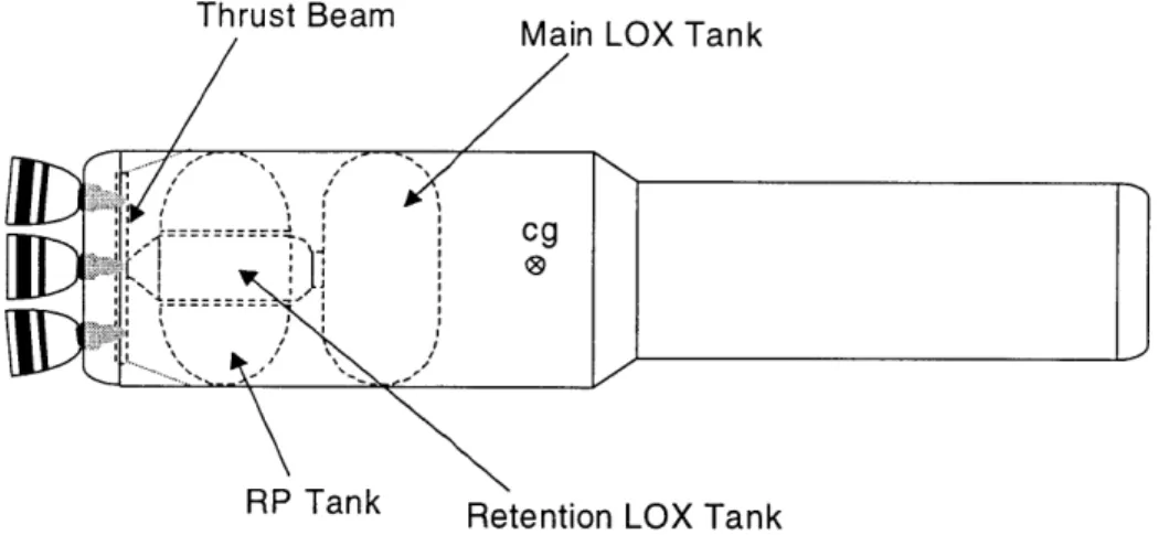
The physical configuration of the stack's boost phase propulsion system is presented in Figure 2.1. As shown, the RP is stored in a donut shaped tank and surrounds the cylindrical LOX retention tank. The main LOX tank is located forward of the other two propellant tanks. The main LOX and RP tank provide the necessary propellant during boost. (Only the main LOX tank is completely

depleted by the end of the ascent phase.) Sufficient RP fuel remains along with the LOX in the retention tank for the LAP return burn.

Thrust Beam _{Main LOX Tank}

RP Tank _{Retention LOX Tank}

Figure 2.1 - Boost Phase Propulsion System Components 2.1.2 Thrust Vector Control Loop

In order to construct a Thrust Vector Control (TVC) loop to design a boost phase control law, the physical system must be translated into a representative model. Figure 2.2 shows the three main components of the K1 TVC.

(33)

1553 Bus Elcrnc1553 Bus

Erta easurement Unit Line Replaceabe Unit

P

Figure 2.2 - K1 TVC Physical Description

The Inertial Measurement Unit (IMU) is composed of accelerometers and gyroscopes that sense the vehicle's rotational and translational accelerations. The IMU also integrates these measurements to produce pitch angle and pitch rate signals, which it sends to the Electronic Line Replaceable Unit (ELRU) on a standard 1553 bus. The ELRU, among other things, is the attitude control computer. Using references on the desired pitch angle and the information supplied by the IMU, the ELRU calculates necessary thrust vector angles to eliminate any attitude errors. These engine angles are transmitted over the 1553 bus to the Propulsion Line Replaceable Unit (PLRU). The PLRU is composed of all of the propulsion-related elements, such as fuel tankage, feed lines, and actuators. However, the most significant parts from a control design perspective are the Vehicle Motor Control (VMC), and the NK-43 engines. The VMC

translates the control commands from the ELRU into commands for the hydraulic actuators that move the engines. The final and less tangible component of the K1 TVC, is the vehicle itself. The dynamics of the stack (combined first and second stages) translate engine motion into new sensor data for the IMU, which completes the TVC loop.

Propuilsion Line Replaceable

NK-43 Engine Actuator Control

(34)

Attitude Control System

Guidance Pitch Plane 6NK-43 Engine Kistler Launch Vehicle

Pitch Angle Reference _Pitc _AnleControl Law ~ef~r~ec~eActuator 60 ms Lag 2"d Order Linearized Equations of

Dynamics Motion

Inertial Measurement Unit

Figure 2.3 - Representative TVC Loop

The objective of the representative control loop is to characterize adequately the response of the physical system with a series of mathematical approximations. Figure 2.3 shows the control loop realization of the physical system. First, the IMU receives sensor information and provides calculated angular rate and attitude to the ELRU on a 1553 data bus. In order to

characterize the dynamics and computation lags associated with the IMU, a

0.0205 second delay and a 17 Hz low-pass filter have been added to the

feedback [6]. Second, the ELRU is represented by a pitch angle reference and the pitch plane control law. The focus of this thesis is the technique involved with designing the pitch plane control law portion of the ELRU. Third, the PLRU is represented by a mathematical model of the dynamics involved with the hydraulic actuators and a 0.06 second delay, which characterizes the computation and transportation times associated with the forward path from the VMC to the

actuators [6]. Finally, the dynamics of the K1 are represented by a system of linearized Equations of Motion (EOMs).

2.2 Reference Coordinate Frame

Two main coordinate systems served as the reference frames for the development of the K1 mathematical model. The inertial reference frame is fixed, right handed, orthonormal, and centered near the K1 center of gravity (CG). _{The body axis system (Figure 2.4) is similar but free to move. Initially, the}

(35)

two reference frames are aligned with the z-direction axis pointing down. Positive roll, pitch, and yaw rotations are also defined in Figure 2.4.

XB (P (roll)

YB

(pitch) S(yaw) ZB

Figure 2.4 - Body Axis System

2.3 Mathematical Model

2.3.1 Dynamic Effects

The K1 Equations of Motion (EOMs) were derived to include the

disturbance effects of gravity, thrust, Tail-Wags-Dog (TWD), fuel sloshing, and body bending, in addition to simple rigid body motion. Appendix A contains a full derivation of the elastic body, pitch plane EOMs. This set of continuous linear time invariant (LTI) EOMs was developed using a simple approach modeled after that used in the Space Shuttle EOM development [3]. First, the force and

moment equations were derived from free-body diagram analysis. Figure 2.5 presents the pitch plane free-body diagram used in the math model development of thrust, gravity and aerodynamic forces. The specific diagrams for slosh, TWD, and flex are contained in Appendix A. Then, the equations were expanded into steady-state and perturbation elements. Next, appropriate trigonometric

(36)

identities were applied in conjunction with the small angle assumption. Finally, after removing the steady-state terms, a set of LTI EOMs remained.

XB FL cp a V FD cg --- --- * XI FG ZB pF-r Z, +

Figure 2.5 - Pitch Plane Free-Body Diagram

2.3.2 Assumptions and Simplifications

To support the gain-scheduled linear control approach, equations derived for the system model have been linearized about the nominal trajectory.

Specifically, these equations are continuous LTI EOMs, which define

perturbations from trim conditions. However, this approach requires that the dynamics of the system are slowly varying and that perturbations to the system are small in magnitude. It was also assumed that the three engines are not

independently controllable. Therefore, a single engine with properties

characteristic of the three NK-43 engines was used. Body-bending effects on the fuel-sloshing mass were assumed to be negligible as there was no data available on rotational and translational flex coefficients at the slosh nodes. Finally, due to the large difference in magnitude between the steady-state axial acceleration and

(37)

the perturbations to the axial acceleration, the axial disturbance force was also neglected, and the axial force EOM was removed.

2.3.3 Ki Plant Model (Stack)

The set of equations, 2.1 through 2.7, characterize the pitch plane

disturbance response of the K1 vehicle. The simplifications presented in Section

2.3.2 were applied to the final set of pitch plane EOMs in Appendix A, and the

resulting plant model state equations are summarized here.

Vertical Velocity State Equation:

# flex mod es m [Aw + UoAq] =-mgo sin 0OA0 - T cos 8 P(A + Y ayeqj)

j=1 # flex

mod es - mele cos 8P (A8P +

I

yej)

j=4 _(2.1) SqLcpCzq Aq + SqC2.Au+2U 2UO #slosh mass + m s2 + 2;sZ

)

k =1

Pitch Angular Velocity State Equation: #flex

mod es

(px cos

p - pz npo (Ap +oCyeqj)

AqlY = 1 T

j=1 [+ xeqj sin po + Ozeqj cos 6po

#flex mod es + (mele (l cos 5po - pZsin

5po)

-lyye)(A 6

I + Iyj) j=1 SqL C (2.2) + SqLoCMXAda + Cp mq Aq 2U q

#slosh O'sZI Aw + 1Z Aq+ (Wo - 2Ql )I Aq

mass

Lk

- MSk +golsz cosO0

AO

+ 2(IS +k Q0lszk )Zskj

k=1

L

(38)

Slosh Mass State Equation:

ZSk = ± s-A x k Aq~ + (U. + 200lSZk )Aq - go sin

6OA0

- 2o) k -# flex mod es $ qZSk j=1 + Q2Z #flex mod es ro-2 z $Z qj Sk Sk I j=1

Angle of Attack State Equation:

Aw - VA6 cos ao = (U0 - V cos ao) Aq

Flex Mode State Equation:

m -2mwm m -om = 1 # flex modes T I

X

Oxem sin 8P.(A8p + T ejqj)

j=1 m

# flex

- s $zem -Cos po(A,+ Gye q)

j=1 m

#flex

mod es j=1

T Cos 8po - Ipzn 8po) (A6p + Yye

yem m xeqj sin po zeqj cos 8po

m Me₁ m # flex mod es I

X

xem j=1 #flex mod es I

X

zem j=1 qj)

sin 6po (A6P + CYyej)

cos 6Og (A, + ye

# flex

mod es (Y y

o

m ye (lyye - mele (1x Cos 6

p= Mm

-lp sin 6₀p))(Ap p + Gyejqj)

Gyroscopic Output Equations:

qactual - Aqsensed actual _A _sensed #flex mod es -X yygyrosj j=1 # flex mod es - (Yygyrosqj j=1 (2.3) (2.4) (2.5) (2.6) (2.7)

(39)

All the parameters used in equations 2.1 through 2.7 are defined in

Appendix A. The state-space representation of these equations used in design is defined by,

x , ₌_A _xP_{+ BPuP}

6 = C1x, (2.8)

6 = Cp₂xp

The system inputs, up, are gimbal angle and gimbal angular acceleration, and the outputs are obviously pitch angle and pitch rate. The order of the stack model ranges from 2 nd order when all dynamics have been neglect except for rigid body

motion to 2 9th order when all dynamic effects are included.

2.3.4 Additional Control Loop Elements

It is important to present the math models of all the pitch plane control loop elements. A more thorough discussion of these elements and of the control loop structure is provided in Chapters 3 and 5. Unlike the K1 plant model that has time varying parameters, these elements remain essentially constant over the entire flight profile.

Actuator Model

The engine actuators have been modeled as a simple 2nd order spring-mass-damper system consistent with specifications [6]. The actuator differential equation is given by equation 2.9, where the frequency is nominally 25.13 rad/s and the damping coefficient is 0.707.

(+22AoA A6 (2.9)

In order to provide the actuator acceleration information necessary to model TWD, the output equation has been modified to include attitude and angular acceleration information. The resulting state-space representation is,

(40)

xA =AAXA +BAUA

Up _{CAXA +DAUA}

IMU Model

IMU attitude and angular rate have been shown to act like 1st order low-pass filters with a bandwidth of 17 Hz (-100 rad/s) and unit DC gain [6]. Using this guidance, the state-space representations shown by equations 2.11 and 2.12 were implemented in the feedback path for both pitch and pitch rate signals.

= A₀X₀+Boo (2.11) Os = CeXe 6 =A6x6 +B66 (2.12) Os =Cx6

Computational Delay Models

Computation and Transportation delays of 0.06 s and .0205 s are respectively present in both the forward path and feedback path of the control loop [6]. Several different ordered Pade approximations were analyzed for modeling these delays. However, adequate system lag was introduced using only a 1st order Pade approximation. Using MATLAB function pade.m to create

the appropriate system, the following state-space representations were introduced into the control loop:

x60=A 60x60+ B60u _(2.13)

A C60X 0 + Du60

x₂₀, =A20, X2, + B200 (2.14)

(41)

202 = A202 X202 + B202 0 (2.15)

y₃= C20x 20 +D2025S

The system in equation 2.13 is the 0.06 VMC delay in the forward path, and equations 2.14 and 2.15 are the IMU delays in the feedback path. Two separate, but identical, state-space models of the IMU delays were incorporated-one to account for pitch angle and one to account for pitch rate.

2.4 Design Point Selection

2.4.1 Historical Considerations

In developing an MCS framework for point design controller synthesis, a decision was made to formulate the process around a trajectory point that has historically proven to be difficult. Typically, the two most demanding regions of a boost profile are the transonic and maximum dynamic pressure regions. The transonic region is characterized by large fluctuations in the aerodynamic derivative coefficients. These dramatic changes create elevated levels of uncertainty in the linearized equations, and emphasize the importance of a quality controller during this region. The maximum dynamic pressure on the vehicle also places increased importance on controller quality. During this

section of the trajectory, the structural load created by a non-zero angle-of-attack is the most extreme. The size of the load, which is characterized by dynamic pressure and angle-of-attack (Qc), serves as a physical limitation that must be accommodated by the control law. The historical importance of successful control within these two regions immediately identifies them as candidates on which to base the development of an MCS control synthesis framework.

2.4.2 Nominal Boost Phase Profile

In order to apply the pitch plane EOMs summarized in equations 2.1 through 2.7 and begin the process of creating a controller point design, a nominal

(42)

pitch plane profile was generated. The nominal trajectory information applied herein is based on simulation results performed on the UNIX Simulation

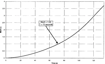
Framework at Draper Laboratory. Using a preliminary Proportional-Derivative (PD) controller data for the pitch plane boost phase was collected to serve as steady-state response information. Figure 2.6 shows the dynamic pressure profile of the nominal trajectory. Figure 2.7 shows the Mach profile of the same trajectory. As alluded to earlier, the critical points of these profiles are

highlighted. The Mach 1.0 point occurs 72 seconds into the boost phase, and the maximum dynamic pressure point occurs at 81 seconds. Because both of these points occur within only seconds of each other, the Mach 1.0 point will serve as the design point during the development of the MCS framework. Using this point, the design process should be capable of being extended to the

remaining design points in the trajectory. Appendix B contains further

information on the nominal pitch plane profile, detailing pitch angle, angle-of-attack, acceleration, and CG location histories.

500 -- - - -400 ---- - - --- - - --- _-Max Q =501.5 lbf/ft^2 300- -- ---- -- - - --- T 81 seconds 200 100 ___ 0 1 0 20 40 60 80 100 120 Time (s)

(43)

3.5- - - - - --- -- --- - --- - - _ - _ - - -3.5 - - - _--- - -- --2.5 _{2.5 --} Mach = 1.00___ ___ -__ -- T =72 seconds_T₌_{72 seconds} 1.5 ___ 1. - __ _ 0 20 40 60 80 100 120 Time (a)

Figure 2.7 - Nominal Trajectory Mach Profile

2.4.3 Design Point System Analysis

A thorough verification of the pitch plane dynamics was performed to

ensure the correctness of the K1 mathematical model. Using the nominal

trajectory data, pole/zero histories of the pitch plane dynamics were compared to the reference models and assessed for discrepancies. Appendix C contains a full description of the pitch-plane, K1 EOM verification for the pitch plane.

The results of this process support using the pitch plane model (equations 2.1 through 2.7) in the development of a control design process. Using this model, the K1 frequency response was generated at the Mach 1.0 design point. Tables 2.1 and 2.2 summarize the parameter values for the K1 model at T = 72 s (Mach 1.0).

(44)

Table 2.1 - LAP Design Model Parameter T M lPX lpz Me leyy le (osix ( six 'sxlx lszlx msIxret (Osix_ret Ssix ret Value (units) 1.0991x106 (Ibf) 1.8565x1 04 (slugs) 1.63x1 07 (slug-ft2₎ -44.468(ft) 0 (ft) 304.125 (slugs) 8023.1 (slug-ft2₎ 4.05 (ft) 3285.2 (slugs) 2.6675 (rad/s) .000087 -23.35 (ft) 0 (ft) 104.824 (slugs) 5.9148 (rad/s) .0027

Table 2.2 - Mode Shape Parameters for first 10 Bending Modes

Flex $xe $ze (ye OIMU (ad/1

Mode (rad/s) 1 -.00069 .000069 .00000052 .0000002 18.47 0.01 2 -.0000016 -.000824 -.00000385 -.0000022 20.77 0.01 3 -.000035 .00371 .000017 .0000122 20.83 0.01 4 .000116 -.00576 -.0000347 -.0000289 24.60 0.01 5 -.000615 .0315 .000212 .000126 24.74 0.01 6 .000255 .00018 .00000119 .00000084 27.71 0.01 7 .000553 -.00187 -.0000273 -.00000838 30.41 0.01 8 .000445 -.0067 -.000273 -.000026 32.26 0.01 9 -.000759 -.00986 -.0000181 -.0000577 32.53 0.01 10 .00054 -.00309 -.00000499 -.0000166 33.28 0.01

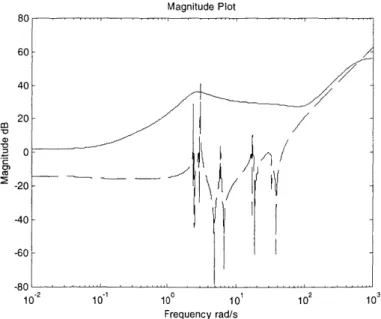
2.5 K1 Frequency Response Analysis

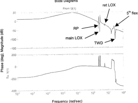
Two types of frequency responses will be used for analysis throughout this thesis. Figure 2.8 presents a Nichols representation of the K1 system model

Isxix ret Iszlx_ret msrp (Osrp srp lsxrp lszrp U0 S L Cza Cma Cmq Uo -33.3214 (ft) 0 (ft) 1340.3 (slugs) 2.3208 (rad/s) .000375 -37.4796 (ft) 0 (ft) 985.9607 (ft/s) 201 (ft2₎ 480 (Ibf/ft2₎ 16 (ft) -.0721 rad .0921 rad1 -34.58 rad1 -.71 deg Parameters

(45)

frequency response. Nichols plots will be used primarily because of their easily interpreted graphical representation of stability and various stability margins. In addition, dynamic effects are more distinguishable when the frequency response

is plotted as magnitude versus phase. Bode plots will also be used to reference specific dynamic effects to points in the frequency spectrum. Figure 2.9 presents a Bode plot of the plant's frequency response. Together, these representations

provide an adequate means of assessing the system dynamics.

Nichols Charts main LOX RP + im 9th flex ret LOX 0 C; . 0 / TWD 5 3C: -2002 0- 10 20

Open-Loop Phase (deg)

An application of robust H₂/H[infinity] control synthesis to launch vehicle ascent by Tyler Nicklaus Hague.