Application of signal analysis techniques to cardiac arrhythmia detection and classification.

APPLICATION OF SIGNAL ANALYSIS TECHNIQUES TO CARDIAC ARRHYTHMIA DETECTION AND CLASSIFICATION

by

JYH-YUN WANG

B.S. in Physics, Fu Jen University, Taiwan 1970

M.S. in Physics, Northeastern University 1973

SUBMITTED IN PARTIAL FULFILLMENT OF THE REQUIREMENTS FOR THE DEGREE OF

MASTER OF SCIENCE

at the

MASSACHUSETTS INSTITUTE OF TECHNOLOGY January, 1976

Signature of Author 6A

Department of Aeronautics and Astronautics, January 26, 1976

Certified b

Accepted by

Thesis Supervisor

A

s -/

Chairman, Departmental Graduate Committee

APPLICATION OF SIGNAL ANALYSIS TECHNIQUES TO CARDIAC ARRHYTHMIA DETECTION AND CLASSIFICATION

by

Jyh-Yun Wang

Submitted to the Department of Aeronautics and Astronautics on January 26, 1976, in partial fulfillment of the requirement for the degree of Master of Science.

ABSTRACT

A completely new approach to develop an automated program for rhythm ana-lysis of electrocardiograms and vectorcardiograms using powerful statistical techniques of sequential estimation and detection theory is studied. The underlying cardiac rhythms are modeled as outputs of low-order linear sto-chastic dynamical systems. The relatively predictable persistent cardiac rhythms are detected and classified by using a multiple model hypothesis testing technique. Detection and classification of the relatively unpre-dictable transient cardiac arrhythmias are performed using a generalized likelihood ratio technique. Both the multiple model hypothesis testing and the generalized likelihood ratio identification techniques are tested extensively on a variety of actual data which includes normal sinus rhythm, bigeminy, trigeminy, PVC, PAC, dropped beat, SA block, tachycardia burst, multiple PVC, and slowing of heart rate. The results indicate that these cardiac events can be identified with great accuracy.

Thesis Supervisor: Alan S. Willsky, Ph.D.

Title: Assistant Professor of Electrical Engineering

-2-I

ACKNOWLEDGMENTS

The author wishes to express his appreciation to his thesis advisor, Professor Alan S. Willsky, for his continued encouragement and constructive advice and comments throughout his thesis research. The author is particularly grateful to Dr. Donald E. Gustafson of the Charles Stark Draper Laboratory, for introducing him to this program and for providing continued assistance, support and encouragement. It was a great pleasure to work with them.

Special thanks go to Colonel M. Lancaster and his other associates at the United States Air Force School of Aerospace Medicine for giving their support and advice on medical matters, and for providing electro-cardiographic records.

Finally, the author wishes to acknowledge the Charles Stark Draper Laboratory whose personnel and facilities contributed greatly to this work.

This thesis was prepared under CSDL Projects 52-65700 and 52-70000, sponsored by the United States Air Force School of Aerospace Medicine through contracts F41609-75-C-0013 and F41609-76-C-0004.

The publication of this work does not constitute approval by the United States Air Force or the Charles Stark Draper Laboratory of the findings or conclusions contained therein. It is published only for the exchange and stimulation of ideas.

TABLE OF CONTENTS

Chapter Page

1

1.1 Principle of Electrocardiography 6 1.2 Computer-Aided Analysis of the Electrocardiogram 9

1.2.1 Background 9

1.2.2 Historical Review ₁₂

1.3 Methods of Approach 15

1.4 Synopsis of Following Chapters 18

2 DATA PREPROCESSING 20

2.1 Baseline Removal 20

2.2 Fiducial Point Detection for the QRS Complex 22 2.3 Algorithm for Fiducial Point Detection 24

2.4 Experiments and Results 28

3 CATEGORIZATION OF CARDIAC ARRHYTHMIAS 48

3.1 Introduction 48

3.2 Persistent Rhythms 49

3.3 Transient Events 51

4 STATISTICAL ANALYSIS OF R-R INTERVAL DATA 55

4.1 Introduction 55

4.2 Analysis ₅₅

4.2.1 Histogram, Sample Mean and Sample

Variance ₅₅

4.2.2 Running Mean and Running Variance 58 4.2.3 Sliding Window Mean, Variance, 61

and Outlier Test

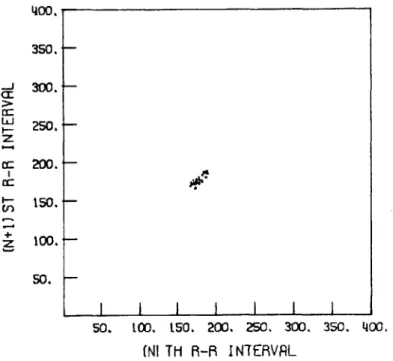
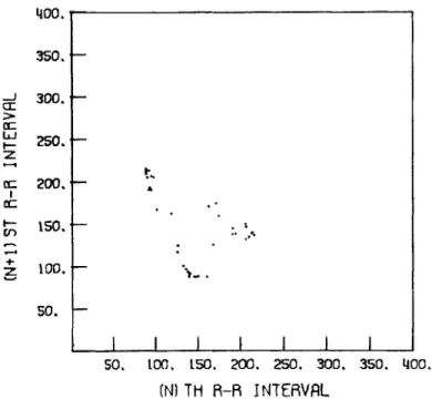
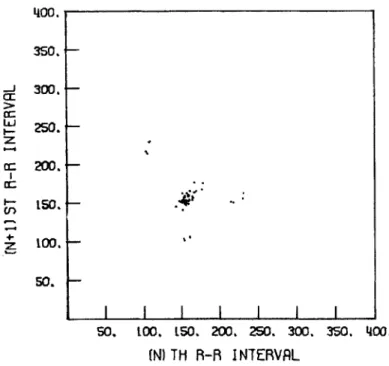
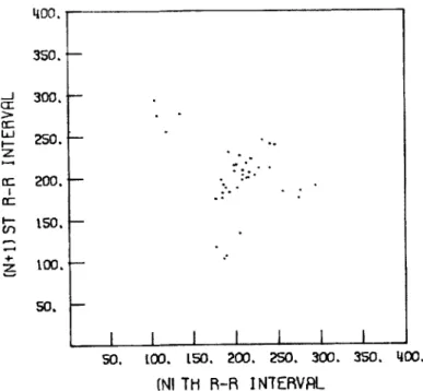
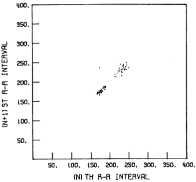
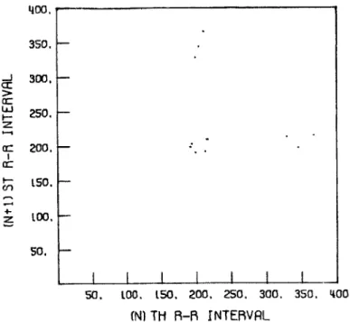
4.2.4 Correlation Functions and Scatter Diagram 64

4.3 Experiments and Results ₇₀

5 _{DYNAMICAL MODELLING OF CARDIAC RHYTHMS BASED ON THEIR 159} R-R INTERVAL CHARACTERISTICS

5.1 Introduction 159

5.2 Dynamical Models for Persistent Rhythms 160 5.3 Dynamical Models for Transient Rhythms 167

Chapter

6 DETECTION AND CLASSIFICATION OF PERSISTENT 172 RHYTHMS

6.1 The Multiple Model Hypothesis Testing

Technique 172

6.2 The Multiple Model Hypothesis Testing 177 Algorithm

6.3 Experiments and Results 186

7 DETECTION AND CLASSIFICATION OF TRANSIENT 254 RHYTHMS

7.1 Generalized Likelihood Ratio Technique 254 7.2 Derivation of GLR Equations

7.2.1 Derivation of Rhythm Signatures 257 7.2.2 Derivation of Likelihood Ratios

and Jump Estimates 264

7.3 Additional Considerations for GLR 273

Computations

7.3.1 GLR Window Width 273

7.3.2 Filter Initialization 275

7.4 Experiments and Results 277

8 CONCLUSIONS AND RECOMMENDATIONS 359

References 365

CHAPTER 1 INTRODUCTION 1.1 Principle of Electrocardiography

It has been known for many years that a measurable amount of potential variations within the electrical field on the body surface is associated with the electrical activity of the heart. As early as

1887, Ludwig and Waller [1] experimented with the capillary electro-scope and recorded this electromotive force from the precordium. In

1899, Wenckebach [2] employed the polygraph to make simple but precise observations of the electrical events of atrial and ventricular acti-vation. Einthoven's description [3], in 1903, of the string galvano-meter for recording the potential variations, stimulated a sudden increase in both clinical and experimental studies of electrocardio-graphy. This type of galvanometer has remained one of the most

frequently used recording method because of its simplicity and porta-bility,although other principles, such as the use of vacuum tube

amplification, have been applied. Recording the potential difference between any two points on the body surface is accomplised by means of electrode from which the current is conducted to the galvanometer of the electrocardiograph via the lead wire, to be returned to the body

by way of a second lead wire and its electrode. In clinical practice twelve leads are usually recorded routinely: (1) three bipolar

extremity leads (standard limb leads), (2) three unipolar extremity leads, and (3) six unipolar precordial chest leads [4]. Using this standard twelve-lead system, the resulting potential difference record is called the Electrocardiogram (ECG).

Biophysical models of the heart and factor analysis of surface potentials have shown that the electrical effects on the surface of the body can largely be accounted for by a single equivalent electrical dipole free to rotate in three dimensions [51-[7]. Under suitable homogeneity assumptions, the components of this equivalent dipole can be estimated by measuring three potential differences in perpendicular directions on the surface of the body, or by resolving non-orthogonal measurements. In practice, the Frank orthogonal lead system which consists of seven leads resolved along mutually orthogonal axes [8],

is the most commonly used for this purpose. A record obtained by the use of this lead system is called a Vectorcardiogram (VCG).

While many differences occur in various leads from the same

subject, and different persons yield distinctive curves, they all tend to conform to a common pattern illustrated in Figure 1.1. The normal electrocardiogram of a cardiac cycle consists of a series of waves arbitrarily designated by Einthoven as the P wave, the QRS complex, and the T wave. When the heart is at rest the electrocardiogram

dis-R

T P

Q

S

plays a straight horizontal line, the so-called iso-electric line or baseline. This baseline represents a constant direct current value produced by the recording device. Alternating current developed with myocardial activity is superimposed upon this baseline and is recorded as upward (positive) or downward (negative) deflections. The baseline may be shifted whenever there is movement of electrodes or a sudden change in skin resistance. In such a case the electrocardio-graphic signal is superimposed upon the baseline variations.

The P wave represents the depolarization wave of the auricular musculature which spreads radially from the sinoauricular (SA) node to the atrioventricular (AV) node. There is a delay in transmission of the impulse at the AV node, represented on the electrocardiogram by the P-R segment. The QRS complex is the depolarization of the ventri-cular musculature. It consists, usually, of an initial downward deflec-tion, the 0 wave, an initial upward deflecdeflec-tion, the R wave, and an

initial downward deflection after the R wave, the S wave. The T wave represents the ventricular repolarization and follows the QRS complex with a delay, the S-T segment, which represents, roughly, the duration of the excited state of the ventricular musculature, or the interval of time between completion of depolarization and the beginning of repolarization of the ventricular musculature (9].

Under pathological conditions the electrocardiogram undergoes some characteristic changes. The various resulting abnormalities in the electrocardiogram may be divided into two groups:

(1) _{disturbances in the cardiac rhythm, and (2) changes in the}

waveform are more or less related to the specific pathological process and its location in the heart, and thus, can be used to describe the state of the working muscle masses. The abnormalities in the order of the heart beat, known as cardiac arrhythmias, yields information concerning the sites and rates of cardiac pacemakers and the impulse propagation through the cardiac conduction system [9]. The electro-cardiogram is the instrument "par excellence" in the diagnosis of the following clinical conditions: myocardial infection, atrial and ventricular hypertrophy, arrhythmias, pericarditis and systemic diseases which affect the heart. A complete analysis of the electrocardiogram should include both the rhythm analysis and the waveform analysis.

1.2 Computer-Aided Analysis of the Electrocardiogram 1.2.1 Background

Due to the high cost of labor, and the large amount of ECG/VCG records to be analyzed, the time available to the interpreting cardio-logist is too limited for taking a multitude of measurements. In addition, due to the limited precision of hand measuring, which does not exceed 0.05 mm, and lack of well-defined criteria for determining the onset and end of waves especially in cases when waves are of low amplitude and have gradual slope, cardiologists are known to differ frequently in their measuring of electrocardiographic events. It is difficult to correlate mentally large numbers of ECG/VCG parameters, and extensive hand calculations for making use of efficient statistical classification techniques are also too time-consuming to be practical.

Careful studies have been made to assess the human variability in ECG interpretation. In one study, the results showed that in

repeated observations of one ECG the same cardiologist did not agree with his own diagnostic statements in 20% of the time, and different

cardiologists did not agree with each other in nearly 25% of the

statements [10]. Another study showed that 7 cardiologists completely agreed in only 28 out of 100 ECG's [11].

The advent of modern computer techniques changed this situation drastically. The unique ability of computers to perform a large number of numerical computations in a very short period of time enables one to apply a variety of mathematical operations for analyzing ECG/VCG records. ECG/VCG analysis from its engineering aspect is also an ideal field for automation. Some of the advantages of using computer-aided analysis of ECG/VCG are given in the following:

(1) Short-term and long-term cost saving.

(2) It become feasible and practical to obtain any number of ECG/VCG measurements. For instance, the slope of the wave at every point can be easily computed. Whether the signals are complex or simple, the measurements will be remarkably precise compared to those obtained manually.

(3) Best utilization of information already available on the scalar or vector electrocardiograms is obtained. Using high fidelity recording equip-ment, the computer can store and repeat the electrical signals of cardiogram; eliminating noise, interference, and other confusing artifacts which present difficulties in analysis.

(4) Application of complex statistical classification procedures no longer represent a limiting factor

(5) It is feasible to perform mass screening of large population groups which is absolutely necessary for the study and control of heart diseases.

Although the computer-aided analysis of ECG/VCG is an attractive one, problems do exist:

(1) In contrast to the human interpreter who possesses high pattern recognition capa-bility, the computer finds this one of the most difficult operations to perform. (2) The tremendous amount of variation that

occurs among subjects, which we would like to classify into the same class, makes it very difficult to invent prac-tical rules that include all instances. (3) For a computer-aided ECG/VCG analysis

pro-gram, the instructions must be listed in an orderly manner and followed precisely during interpretation. In contrast to this orderly, predetermined logical process, the human interpreter has the opportunity to review the record for any amount of time limited only by his own needs. He may review the data randomly, and even correct his initial diagnosis subject to further reviews.

(4) It is very difficult for the computer to identify the P waves, which have low am-plitude and gradual slope, and thus may be buried in noise or masked by ventricular activity. This is also true of other

1.2.2 Historical Review

The concept of computerized analysis of the ECG/VCG is not new. The requirements for practical clinical applications of such programs include two parts: (1) analysis of cardiac rhythm, and (2) analysis of the contour or waveform of the complexes. Starting in the late 1950's there have been numerous efforts to automate the analysis of

ECG/VCG's, resulting in many computer-aided programs for ECG/VCG ana-lysis being used and developed [12]-[27]. Pattern recognition in these programs are almost exclusively done using a heirarchical com-puter logic structure. Much time is spent checking validity of the data, correcting measurement errors, and extrapolating for missing data. These tests are deterministic in that specific thresholds are

set for the various tests, rather than statistical, wherein probabi-listic statements are given based on statistical models of the temporal patterns. Thus, these schemes involve very complex logic structure which are difficult to debug and to modify. Another drawback in using

the logic tree structure is the limitation of the rhythm analysis

program in their assignment of severity levels. For example, arbitrary terms such as "severe", "mild", and "regular" are used. Thus, in

spite of the amount of wo'rk done on this problem, the problem of com-puter-aided analysis of ECG/VCG is not yet completely solved.

Recent comparative studies on the performance of the available programs have indicated that the IBM program was the best overall [28]. On an overall basis, the program had a detection rate of 94.6% on a total of 1150 waveforms tested. However, the rate of correct identi-fication was lower than this detection rate, because some of the arrhythmias detected by the program were assigned to "undetermined

rhythm" by the final identification logic. The program performed even worst on ventricular arrhythmias, for which the detection rate was only 86%. In the reproducibility study, the results showed that using two different digital representations of the same analog ECG record, the output rhythm statements generated by this program did not agree with each other about 10% of the time. It would appear that available programs are too highly tuned in that some features used

for diagnosis actually contain more noise than information.

In more recent years, a variety of statistical analysis procedures for ECG/VCG analysis were studied to improve the performance of de-tection and classification for arrhythmias. Gersch, et al. [29),[30] transformed a sequence of 100 or 200 R-R intervals into a three-symbol

(namely, short, regular, and long R-R interval) Markov chain sequence. The probability that the observed sequence was generated by each set of prototype models characteristic of different arrhythmia classes, was computed. That prototype corresponding to the largest probability of generating the observed sequence was classified as the disorder.

The disorders considered were atrial fibrillation, PVC and PAC, bige-miny, sinus tachycardia with occasional bigeminy , sinus tachycardia,

and ventricular tachycardia. Tests of this approach on patients with atrial fibrillation (AF) and atrial fibrillation with occasional PVC's (AFOCC) showed that 4 out of 15 AF records were misclassified as AFOCC using 200 heart-beats. The performance was worst when using 100 heat-beats. Pipberger, et al. [31] applied linear discriminat function analysis to training and independent sets of three common arrhythmias (namely, normal sinus rhythm, sinus rhythm plus premature beats, and atrial fibrillation) using R-R interval information only.

On an overall basis, this approach correctly classified 85% of the records tested. The performance for the premature beat classification was the worst, for which a correct identification rate of only 66% was obtained.

All the above statistical analysis procedures for classification have used fixed sample tests. Among the problems with a fixed sample test is the -possibility that if the sample size is too large then a transient phenomenon may go undetected due to the large number of normal beats used in the average. Tsui and Wong [32] studied the

feasibility of utilizing Wald's sequential probability test in cardiac rhythm classification. It has provisions for controlling error rate

than sample size. The expected number of observations under pairwise testing of three selected rhythm classes (atrial fibrillation, normal sinus rhythm, and premature atrial and ventricular contractions) as a function of error rate were shown. However, no test of this approach on actual ECG data was given.

It is important to point out that, on an overall basis, arrhythmias were the greatest source of program errors of the three programs

tested (IBM-1971, PHS-D, Mayo-1968) by Bailey, et al. [28]. The im-portance of the identification of arrhythmias is further underlined by the increasing recognition of the role of arrhythmias as a cause of sudden death [33]. Further, the reproducibility results of Bailey, et al. indicate that more robust computer algorithms are needed, and the statistical results suggest that more powerful statis-tical techniques should be used. These facts have provided much of the motivation for the work of developing an automated detection and classification program for rhythm analysis of ECG/VCG studied here.

-14-1.3 Methods of Approach

The problem of automated arrhythmia analysis is, simply put, the problem of adequately reproducing the pattern recognition capabilities of the cardiologist. This problem may be only partially solvable, given the complexity of human pattern recognition capabilities and the

limitations of even the most advanced computers. It seems fair to say that, given the exact timing of P waves and QRS complexes, together with gross descriptions of these waveforms, that arrhythmia diagnosis would be considerably simplified, since the electrophysiological

me-chanisms responsible for a large number of arrhythmia patterns have been described satisfactorily [34]. Theoretically at least, powerful

pattern recognition techniques could then be brought to bear on the problem.

The techniques proposed in this research for arrhythmia detection and classification explicitly take into account uncertainties within each arrhythmia class in a systematic manner by using the very powerful statistical techniques of modern estimation and detection theory.

This approach differs significantly from previous approaches to rhythm analysis in three ways; (1) the underlying rhythms are modeled as outputs of linear stochastic dynamical systems (2) rhythm classifi-cation will be done by hypothesis testing to find the most likely operating system, (3) unpredicted disturbances will be detected using a generalized likelihood ratio technique. Thus, the emphasis is on

statistical modeling and testing of the data.

This approach has several advantages. First, since beat-to-beat variations are present and the wave intervals are never exactly regular, uncertainty has to be accommodated in any rhythm analysis scheme.

This can best be done by first obtaining detailed statistical infor-mation from actual data, which is readily available and quite exten-sive. Given a comprehensive statistical analysis of such data, it is natural to attempt to use it in the best possible manner. This can be done, for example, by trying to match the data to some dynamical model. Thus, if extensive correlation data were available and diagnostically significant, it would be feasible to construct dynamical models with the identical correlation characteristics. One can then bring the powerful techniques of sequential estimation and detection theory into action.

Alternatively, since the temporal patterns of many types of arrhythmias are known, a dynamical model may be subsumed for each "dynamically different" class. The parameters of the models can then be selected to best match the statistical characteristics of the model to the observed data. This approach has been taken in the present research and is covered in detail in subsequent chapters.

Of all of the data that can be obtained from an ECG or VCG, R-R interval data is by far the easiest to obtain and the "cleanest" in the sense of being almost error free. Such data possesses the highest "signal-to-noise ratio" and thus provides the most reliable information. On the other hand, data such as P-R and P-P intervals are inherently more noisy, as the detection of the smaller P waves introduces more errors. Considering this point, we have adopted the point of view that our first task is to understand fully the content of the more accurate R-R interval data. That is, we wish to deter-mine precisely what information concerning arrhythmias is contained in R-R data and then to determine how to best extract this information

-16-from the R-R intervals.

Our work along this direction has several natural subdivisions: (1) The Categorization of Arrhythmias - The determination of how various types of arrhythmic behavior manifest themselves in the ob-served signal. This involves the explicit determination of how various arrhythmias affect R-R interval histories (we do not categorize

the effects of arrhythmias on other observable quantities, such as P-R intervals, P-P intervals, shapes of QRS complexes, etc.; because, for the purpose of this initial study we are mostly concerned with the R-R data). (2) Statistical Analysis of Arrhythmic R-R data -The purpose of this task is to obtain further and more quantitative information about the manifestation of various arrhythmias. Certain simple statistics related to the R-R data are computed, and these statistics can be used either to identify certain arrhythmias or to provide useful inputs in the design of more sophisticated mathematical models. (3) Determination of Dynamic Models for the Generation of R-R Interval Data for Different Arrhythmias - Based on the information in (1) and (2), we can obtain relatively simple dynamic models that generate R-R intervals with the desired statistical properties. The purpose of this task is to construct models to which we can apply the powerful tools of sequential estimation, detection, and hypothesis testing. (4) The Development and Testing of Estimation, Detection, and Hypothesis Testing Algorithms for Arrhythmia Detection Based on

R-R Data - We apply several signal processing techniques to the mathematical models developed in (3).

1.4 Synopsis of Following Chapters

In Chapter 2, an algorithm for fiducial point detection of the

QRS

The categorization of arrhythmias into different distinctive classes is the subject of Chapter 3. This involves the determination of how various types of arrhythmias manifest themselves in the observed

signal, and how various arrhythmias affect the

R-R

Based on the information obtained in Chapters 3 and 4, we deter-mine the dynamical models for the generation of R-P interval data for different arrhythmias in Chapter 5. The purpose of this task is to construct models to which we can apply the powerful statistical analysis tools for detection and classification.

In Chapter 6, the multiple model hypothesis testing algorithm for the detection and classification of persistent rhythms is discussed. Numerical results obtained using actual data are presented. The generalized likelihood ratio detector system for the detection and classification of the transient rhythms is studied in Chapter 7. The necessary GLR equations are derived in detail. Actual data are tested, and the results are presented. Finally, some further discussion and conclusions are qiven in Chapter 8. Several. areas which need further research are also pointed out, and discussed.

All the data used in the tests were digitized at a rate of 250 samples per second, and were provided by USAF/SAM personnel. The computer used to remove the baseline drifts, to locate fiducial point for the QRS complex, and to perform the statistical analysis, was a Nova 2 minicomputer. An IBM/360 computer was used for

CHAPTER 2 DATA PREPROCESSING

Data preprocessing refers herein to the sequence of steps required to obtain the R-R interval sequence from the digitized ECG/VCG record being processed. The preprocessor may be conveniently divided into two steps: (1) remove the low frequency baseline drifts, (2) detect the fiducial points of QRS complexes. These are discussed separately in the following sections.

2.1 Baseline Removal

A crucial step in the computer analysis of ECG/VCG's is the re-moval of low frequency baseline drifts. These disturbances can be quite severe and, if not eliminated, can cause significant errors in fiducial point detection and area computation of the QRS complex, which will be used in arrhythmia detection and classification. The slow varying baseline drift is caused by a combination of factors

including:

(1) DC bias of the ECG/VCG output amplifiers (2) slow changes in temperature

(3) coding/decoding mismatch of the FM tape recording (4) variations in tape speed during data digitization (5) electrode polarization changes

(6) geometric changes of torso due to

respiration

For the present purposes, the baseline will be defined as any unwanted low frequency components of the measured cardiographic sig-nals. Let the measured signal at time t be m(i) and denote the underlying cardiographic signal by v(i). Then,

-20-m(i)

v(i)

base-line estimator, which will take the measured signal m(i) as input and give an estimated baseline b(i) as output. Then we can get the

under-lying cardiographic signal v(i) by subtracting the estimated baseline b(i) from the measured signal m i). The structure of this recursive baseline removal process is illustrated in Figure 2.1.

Baseline Removal Filter

M)

--Estimator

Figure 2.1 Recursive Baseline Removal Process

Several recursive baseline removal processes have been designed and tried in [353, [36]. The results showed that an efficient data preprocessor can best be realized by using a moving average non-causal filter for baseline removal. It is further tested in [37] on

arrhythmic data. The experimental data indicate that very little dia-gnostic information is lost. Since the problem of baseline removal has been studied in detail in [35]-[37], no further discussion is given here.

2.2 Fiducial Point Detection for the QRS Complex

The high slope segments of the QRS complex relative to the re-mainder of the waveform appear to be the most reliable indicator to identify this complex. In order to have a well defined fiducial point for the QRS complex, we use the maximum startup slope point or the maximum slope point before the maximum amplitude of the R wave as the fiducial point (see Figure 2.2). The maximum slope at the fiducial point varies markedly from lead to lead. However, most of the QRS complexes on a given lead have a higher slope at the fiducial point than any part of the P and T waves in that lead. Accordingly, the first step in detecting the fiducial point is to find the slope for each lead which distinguishes P's and T's from QRS's.

Although this method is generally quite reliable, some problems do exist. Occasionally a small number of aberrant QRS complexes are present in a record. The maximum slope at the fiducial point on these QRS complexes may be markedly lower than the maximum slope on the complexes representing the dominant rhythm, and comparable to the high

slope parts of the T waves. In this case it is not possible to find a slope which will distinguish all of the T waves from the QRS complexes. In order to detect all the QRS complexes, we therefore have to set the slope threshold at a very low value. Although we will be able to detect all the QRS complexes by doing this, at the same time we will also detect those T waves which have their maximum slopes greater than the slope threshold. The easiest way to avoid this difficulty is to

-22-R P

s

1T

\7

Time

Figure 2.2 Fiducial Point Detection T Time w ro :1 4J .H "i 04 A 04 01 I

skip a selected number of data points after the fiducial point is de-tected. We choose the number of data points to be skipped to insure

skipping of the T wave, yet small enough so as not to miss any QRS complexes.

Another problem caused by using the low slope threshold is that we will detect noise bursts which have slopes greater than the slope threshold and which are not in the region skipped after the detection of the fiducial point. Since these have amplitudes much lower than the amplitudes at the fiducial points, we can thus reject them by

re-quiring that the fiducial point should also satisfy the condition that the product of its amplitude and slope be greater than a positive

threshold. This condition will not only reject noise bursts, but also insure that the fiducial points of the R waves detected are at the points before the maximum amplitudes of the R waves, since we require

slope times amplitude to be positive.

2.3 Algorithm for Fiducial Point Detection

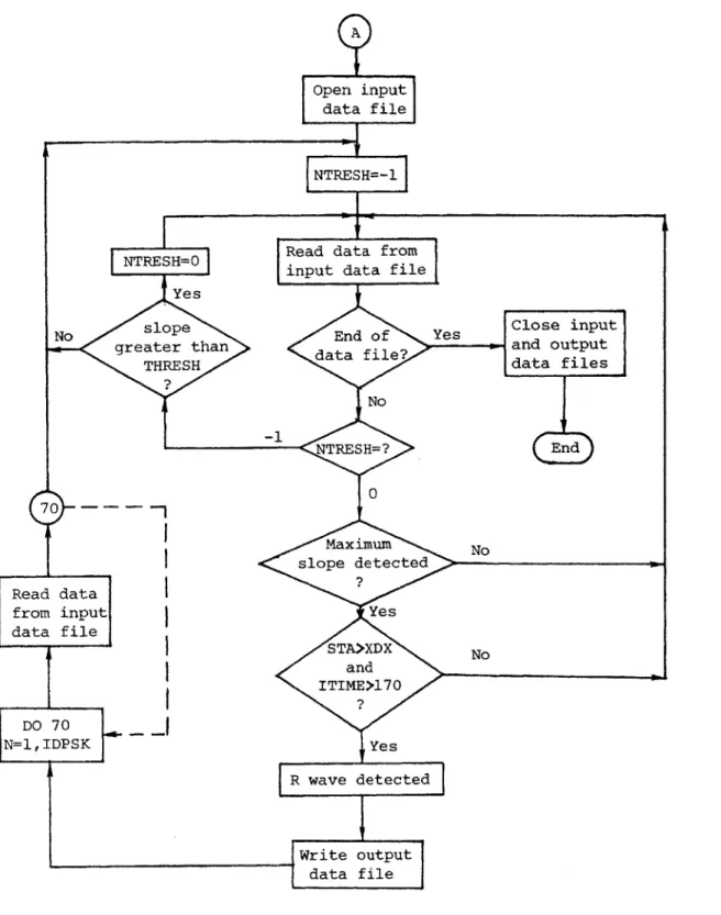
A program, RRFILE, has been developed based on the conceptdes-cribed above for detecting the fiducial points of the QRS complexes for both the arrhythmic and non-arrhythmic data from which the low frequency baseline shifts have been removed. A detailed description of the

algorithm is given in the following, and a flow chart of this program is shown in Figures 2.3(a) and 2.3(b).

First, three data points are read into REM(l), REM(2) and REM(3). The slope of a best fit straight line over these three points is

calculated as: REM(3) - REM(l). The window REM moves forward by dropping its trailing point REM(l), shifting REM(2) to REM(l), etc.,

-24-TStart

Open input data file

N= 0

Read data from input data file

REM(l), REM(2), REM(3) Eor max.

a value

slope N = N +

1

00

data

of inpu data Yas _{C ile}

file? No No s N>500? _En Yes Set slope threshold TRESH equal to TREM*PERC Close input data file A

Figure 2.3(a) Flow Chart for Program RRFILE Search absolut of the TREM ov first 5 points

Open

data f ile

NTRESH=-l

NTRESH=O Read data from

input

No soeEnd

o

output

THRESH data files

No - NTRESH=?Ed

0

from input Yes

data file

STA>XDX

output

Figure 2.3(b) Flow Chart for Program RRFILE

-26-and reading in a new data point as REM(3). The maximum absolute value of the slope, TREM, over the first 500 data points in the input data

file is searched. The slope threshold, TRESH, is then set at a

certain percent PERC of the maximum absolute value of the slope TREM. The value of PERC is an adjustable parameter.

Once the slope threshold is set for this record, we can start searching for the fiducial points from the very beginning of this input data file. When the absolute value of the slope TSUM is greater than the slope threshold TRESH, the maximum slope is searched. This maximum slope point is not the fiducial point of an R wave, unless the product, STA, of its amplitude REM(3) and slope TSUM is greater than a threshold XDX. The value of XDX is a design parameter.

Finally, we require ITIME, the point where a fiducial point is detected, to be greater than 170 before we can declare that an R wave has been detected. The reason for imposing this condition is due to the fact that some records

may

A safe way to avoid this problem is to neglect the fiducial point

detected within the first 50 data points, which is greater than the

width of a QRS complex. All the input data files used in this program must have their baseline shifts removed first. That is, the input to the program RRFILE is the output data file from the baseline removal filter BSLNFT, in which a moving window average is used to estimate the baseline. The baseline at the midpoint of the overall window is

estimated as the average of all the data pr4nts within this window. Thus, at the start of a record no baseline estimates can be made for the first 120 data points which are used to fill the window. Hence a

value of zero is assigned to the first 120 output data points for the

baseline removal filter. Therefore, in order to avoid false detection

we neglect the fiducial point detected within the first 170 data

points in a record.

When a fiducial point is detected, a selected number of data

points IDPSK are not searched for R waves. This will not only skip

the high slope part of the T waves but also speed up the overall

pro-cessing. The value of IDPSK is a design parameter.

2.4 Experiments and Results

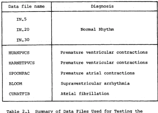
The algorithm for R wave detection RRFILE was tested for both

arrhythmic and non-arrhythmic data. A summary of all these data

files is given in Table 2.1.

Data file name

Diagnosis

IN.5

IN.20

Normal

Rhythm

IN,30

HUANPVCS

Premature ventricular contractions

HARNETPVCS

Premature ventricular contractions

SPOONPAC

Premature atrial contractions

BLOOM

Supraventricular arrhythmia

CUNATFIB

Atrial fibrillation

Table 2.1 Summary of Data Files Used for Testing the Fiducial Point Detector RRFILE

The objective of this test was to determine whether the algorithm des-cribed in Section 2.3 could detect all of the R waves and reject all T waves and noises in each record for a proper choice of the parameters PERC, XDXand IDPSK, where PERC is the percentage of the maximum ab-solute value of the slope TREM over the first 500 data points for the slope threshold TRESH, (TRESH=TREM*PERC), XDX is the slope times ampli-tude threshold for REM(3)*TSUM, and IDPSK is the number of data points skipped after a fiducial point is detected. We also wished to find a set (or sets) of numbers for the parameters PERC, XDX and IDPSK which are good in the sense that no R waves are missed in any of the data

files we have on hand (see Table 2.1). This will aid in our evaluating the robustness of the detector with respect to these parameters.

The input data files to the R wave detector RRFILE were the third lead of those in Table 2.1, from which the baseline shifts have been removed, and the output data files were the R-R intervals detected in each lead. A total of 1,000 sampling data points (250 data points

=1 second) in the third lead of all the arrhythmia data files both before and after the baseline shifts have been removed are shown in

Figures 2.4 - 2.8). From these figures we can see that there are aberrant R waves present in all these data files. Note also that the filtered waveforms appear unaffected from a diagnostic viewpoint. All these data files were tested individually at first for different values of parameters. The R waves detected for each different set of para-meters were then checked visually with the data files, which were dis-played on the Tektronics 4010 digital display. Finally, a satisfactory set of values for the parameters were found, which were good for all the data files being tested. These are given in the following:

PERC =

0.20

XDX =

3,000

IDPSK

=

70

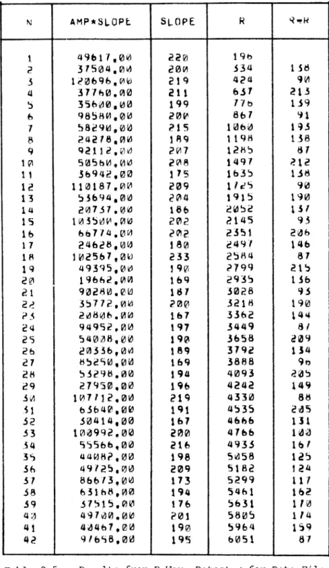
The results are given in Tables 2.2-2.9 for all the data files in Table 2.1. The fourth and fifth columns give the fiducial point

detected and the intervals between the two consecutive fiducial points (or the so called R-R intervals), respectively. We also give the slope and slope* amplitude at the fiducial point in column two and three, respectively. The R-R interval data in column five is in the output data file from program RRFILE. This R-R interval data file will be used in subsequent chapters for arrhythmia analysis.

In this section we have developed a simple procedure for the determination of fiducial points of the QRS complexes. Although good performance was obtained for the data files tested, more data should be tested to evaluate this fiducial point detector in a wide variety of situations. These tests will either be used to adjust parameters of the present detector, or suggest more robust detector designs.

1400. 1500. 1600. a00.

V.

A

Figure 2.4(a) Unfiltered Data File HUANPVCS

L200.

L300.

L500.

1600.

V.

v

1600.

L900.

A

Figure 2.4(b) Filtered Data File HUANPVCS

1000.

1t00.

1900.

I ffo.

ILOU.

1200.

1200.

'AWW4 !%%

. ,e

4000.

4100.

4300.

.W*00

V

Figure 2.5(a) Unfiltered Data File HARNETPVCS

4000. 4100. 4200. 4300. W400, 4500. 4600. 4W. 4WD, 4900.

5000.

_______________ 3~ Lb ~

Figure 2.5(b) Filtered Data File HARNETPVCS .1

P~f I-

_WI

.sA m&& L. Ao j.L Lo ww.- pow% dofts.

? :"&%

JAN A ftL

7600. 7700. 7800. 7900. 8000. VI ._I £ t

I4~

1-V

Figure 2.6(a) Unfiltered Data File SPOONPAC

7000. 7100. 7200. 7300. 7400. 7500. II. 7600. 7700. I. V 7800. 7900. 8000. V

Figure 2.6(b) Filtered Data File SPOONPAC

r - I --. %% 1 0% if - &% -10

1000. 1 L00. 1200. 1300. 1400.

1500.

1800.

A A

Figure 2.7(a) Unfiltered Data File BLOOM

1000. 1100. 120. 1300. 1400. 150. 1600. 1700.

1600,

1900.

I. y

W.

-Figure 2.7(b) Filtered Data File BLOOM

?Soo V

I'?

s. I

a I ..

1400,

1500.

1600.

1700.

LOW.

1900.

_*-~-

-~-I.'

Figure 2.8(a) Unfiltered Data File CUNATFIB

1000.

100.

L700.

Lew.

L900.

1.1 I I I I

4.

Figure 2.8(b) Filtered Data File CUNATFIB

*v. w.

~?4L

*1

4

N

AMP*SLOPE

J8LQPj

R

ROR

1

309222,00

486

343

2

142400,00

467

524

181

3

289014,00

517

706

182

4

335369,00

524

893

18

5

410010,00

503

1081

188

6

302316,00

491

1266

185

7

251758,00

486

1446

10

8

383176,00

518

1629

183

9

318708,00

528

1814

185

10

371700,00

514

2001

187

11

302670,00

506

2186

185

12

179740,00

463

2366

%80

13

420332,00

479

2549

183

14

384524,00

522

2735

186

15

240672,00

514

2921

186

16

167268,00

479

3101

180

17

254380,00

477

3275

174

18

362604,00

509

3448

173

19

250332,00

534

3624

176

20

289333,00

529

3804

180

21

314730.00

475

3980

176

22

377762,00

451

4153

173

4

23

284400,00

526

4330

177

24

387660,00

507

4506

176

25

272847,00

520

4683

177

26

18732e,00

479

4854

171

27

315792,00

474

5019

165

28

322848,00

524

5187

168

29

356580,00

536

5357

170

30

227416,00

496

5533

176

31

375221,00

454

5705

172

32

234720,00

493

5871

166

33

197358,00

488

6044

173

34

292734,00

545

6218

174

35

237870,00

513

6395

177

36

307572.00

506

6567

172

37

338845,00

473

6133

166

38

283974,00

506

b903

170

39

355200,00

530

7075

172

40

324401,00

544

7248

173

41

363540,00

470

7421

173

42

283745,00

483

7592

171

43

174523,00

467

7763

171

Table 2.2 Results from R Wave Detector for Data File IN.5

N

AMP*SLOPE

SLOPE

R

RwR

I

b38420,00

639

224

2

601198,00

631

423

199

3

700036,00

636

629

206

4

624162,00

630

834

245

5

625719,00

634

1028

194

6

678700,00

619

1226

198

7

658125,00

635

1431

205

8

642178,00

622

1634

203

9

635680,00

653

1828

194

10

646323,00

625

2022

194

11

600392,00

632

2222

200

12

666357,00

633

2422

200

13

583128,00

630

2614

192

14

522886,00

629

2807

193

15

510960,00

631

3006

199

16

656051,00

632

3202

196

17

607910,00

629

3387

185

18

554228,00

630

357!

190

19

b25443,00

645

3177

200

20

638352,00

655

3980

203

21

538248,00

622

"176

196

22

500185,00

636

4378

202

23

612315,00

633

4586

208

24

605402,00

640

4790

204

25

b02141,00

624

4989

199

26

525800,00

626

5194

205

27

522110,00

635

5398

204

28

585972,00

641

5593

195

29

590187,00

636

5791

198

30

604144,00

641

5997

206

31

685035,00

661

6204

207

32

544208,00

638

6405

201

33

609224,00

642

6613

208

34

548886,00

640

6828

215

35

593388,00

637

7038

210

36

578716,00

617

7239

201

N

AMP*SLOPE

SLOPE

R

R

1

575901,00

647

376

2

601650,00

606

612

236

3

557118,00

619

854

242

4

579723,00

614

1093

239

5

550745,00

652

1325

232

6

660050,00

659

1548

223

7

304010,00

594

1778

230

8

461610,00

600

2009

231

9

608854,00

637

2239

230

10

670735,00

680

2464

225

11

653016,00

626

2692

228

12

556665,00

587

2936

244

13

624193,00

624

3185

249

14

562100,00

662

3420

235

15

475295,00

6b0

3655

235

16

474240,00

593

3899

244

17

616701,00

607

4142

243

18

664796,00

640

4373

231

19

586440,00

663

4596

223

20

620730,00

632

4821

225

21

540855,00

605

5055

234

22

571340,00

611

5294

239

23

638400,00

663

5526

232

24

567120,00

629

5758

232

25

567862,00

601

5998

240

26

544840,00

61?

6235

237

27

463246,00

632

6465

230

28

b53646,00

683

6680

215

29

592620,00

682

6892

212

30

601620,00

614

7105

213

31

529440,00

553

7323

218

32

667454,00

657

7544

221

33

b40646,00

656

7771

221

Table 2.4 Results from R Wave Detector for Data File IN.30

-38-4

N

AMP*SOPL

SLOPE

R

49b17,00

22l

19h

2

31504,00

200

334

18

3

1;0696,00

219

424

90

4

37760,00

211

637

213

5

35610,00

199

77t>

139

6

98580,00

20V

867

91

7

58290,00

215

1060

193

8

24218,00

189

1198

138

9

9211200

207

12h5

87

10

505hO.00

208

1497

212

11

36942,00

175

1635

138

12

110187000

209

tiles

90

13

53694,00

204

1915

190

14

20731.00

186

2052

137

15

103500,00

202

2145

93

16

66714.00

202

2351

206

17

24628,00

180

2491

146

18

102567,00

233

2584

87

19

49395,00

19V

2799

215

20

19662,00

169

2935

156

21

90280.00

187

3028

93

2?

35772,00

200

3218

190

P3

20806.00

167

3362

144

24

94952,00

197

3449

8?

25

54008,00

190

3658

209

26

20336,00

189

3792

134

27

85290,00

169

3888

90

28

53298.00

194

4093

P45

29

27950,00

196

4242

149

3

107112.00

219

4330

88

.i

63640,00

191

4535

205

32

30414,00

167

4666

131

33

100992,00

200

4766

100

34

55566,00

216

4935

161

35

44082,00

198

5058

125

36

49125,00

209

5182

124

37

86613,00

173

5299

111

38

63168,00

194

5461

162

39

31515,00

176

5631

110

40

49700.00

P01

5805

114

41

40

00

190

5964

159

42

91698,00

19S

6051

87

Table 2.5 Results from R Wave Detert+jr for Data File HUANPVCS

N

AMP*SLOPL

SLOPE

R

RwR

1

187192,014

116

227

2

14833,00

98

381

154

5

16791,00

Ii6

533

152

4

12388,00

101

692

159

5

3276,00

45

798

106

6

15662,00

115

1028

230

7

11255,00

110

1190

162

1415,100

100

1348

158

9

5280,00

108

1502

154

10

4312,00

57

1649

147

11

18291,00

101

1800

151

12

26924,100

126

1951

151

13

32112,00

133

2105

154

14

28416,00

140

2257

152

15

34075,00

158

2416

159

lb

24252,00

136

2581

165

17

38148.00

165

2744

163

18

29555,00

131

2901

157

19

30702,00

150

3061

160

20

10595,00

65

3166

105

21

30492,00

135

3395

229

2p

24910,00

152

3550

155

23

31255,00

142

3712

162

24

28320,00

150

3866

154

25

21144,00

146

4016

ISO

26

28896,00

150

4170

154

27

27132,00

144

4323

153

28

27664,00

146

4471

148

29

23552,00

146

4624

153

3P

3132,00

38

4725

101

31

32562,00

135

4942

21r

32

30222,100

141

5092

150

33

25864,00

135

5246

154

34

16566,00

133

5395

149

35

30702,00

148

5545

150

36

21156,00

147

5686

141

37

23544,00

128

5831

145

38

1176,00

107

5983

152

39

4968,00

65

6086

103

40

24696,00

126

6300

214

41

30226,00

136

6451

151

42

25338,00

147

6602

151

43

29348,00

116

6759

157

Table 2.6(a) Results from R Wave Detector for Data File HARNETPVCS

-40-Table 2.6(b) _{Results from R Wave Detector for Data} File HAPIIETPVCS

AMP*SLOPE

SLOPE

R

i"

44

15453,00

112

6911

152

45

2592t,0

148

7068

157

46

32508,00

132

72?6

158

41

253122,00

t39

7315

149

48

16920,00

M1

1537

162

49

24300900

123

7695

158

50

18948,00

131

1860

165

131

2RP2,00

130

803b

116

52

20384,00

140

8211

175

53

2201$,0o

140

8378

16?

54

288M0.0O

136

8544

165