1
Supporting Information for
Energy Level Alignment at Hybridized Organic-Metal Interfaces: The Role
of Many-Electron Effects
Yifeng Chen1, Isaac Tamblyn2,3 and Su Ying Quek1,4*
1Centre for Advanced 2D Materials and Graphene Research Centre, National University
of Singapore, 6 Science Drive 2, Singapore 117542
2National Research Council of Canada, 100 Sussex Drive, Ottawa, Ontario, K1A 0R6,
Canada
3Department of Physics, University of Ontario Institute of Technology, Oshawa, Ontario,
L1H 7K4
4Department of Physics, National University of Singapore, 2 Science Drive 3, Singapore
117551
*: Corresponding author: phyqsy@nus.edu.sg
Table of contents
1) General details on computational methods used
2) Details of molecular GW self-energy projection calculation 3) GW convergence of Au(111) work function
4) GW convergence of gas-phase molecular orbital levels
5) Off-diagonal elements of GW self-energy evaluated in the BDA MO basis for Geometry 4
6) Off-diagonal elements of GW self-energy evaluated in the BP MO basis for Geometry 7
7) Off-diagonal elements of GW self-energy evaluated in the BT MO basis for Geometry 11
8) Other geometries considered for BDA molecular layer on Au(111) 9) Geometries of metal/molecule/metal junction structures
10) Decomposed self-energy contributions of MO levels from GW versus static-COHSEX results: Comprehensive result
11) Charge rearrangement and binding energy upon molecular adsorption on the Au(111) surface
2 12) Molecule/metal slab geometric parameters
13) DFT and GW bandstructure for the BDA layer as in Geo. 4
14) GW projected molecular level dispersion across the Brillouin zone 15) Calculated image charge correction energy for the hybridized slabs
16) Projected density of states together with our DFT starting points marked for Geo.’s 1-11 investigated in this work.
17) Table S11 summarizing all data
1) General details on computational methods used
Geometry optimization was performed using both VASP [1] and Quantum-ESPRESSO [2] (Q.E.). To account for long-range van der Waals interactions, we used both the Grimme’s PBE-D2 method [3] (as implemented in Quantum Espresso) and the van der Waals density functional (vdW-DF2, optB86b) [4,5] (as implemented in VASP); key geometric parameters are given in Table S8 for all geometries in this work. Geometry 3 was built from experimental information [6] and relaxed in VASP with vdW-DF2 (optB86b), while the BDA linear chain model was provided by Guo Li [7]. Bader charge analysis was performed on total charge densities produced by Q.E. with the UTexas code [8].
GW calculations were done using the BerkeleyGW package [9], with DFT wavefunction input taken from Q.E. using a norm-conserving pseudopotential, PBE
exchange-correlation functional, 60 Ry kinetic energy cutoff, and 10-6 Ry convergence threshold.
Due to the spatial overlap of semi-core and valence wavefunctions in Au [10], we used a 19-electron Au pseudopotential in our GW calculations. A vacuum size of at least 13 Å between periodic slabs was used, and the Coulomb interactions between supercells were truncated with the “cell_slab truncation” and “cell_box truncation” methods. We
employed a 20 Ry energy cutoff for the epsilon matrix (epsilon cutoff), as well as a 20 Ry
screened Coulomb cutoff. We used 5000 bands for 15x15x15 Å3 cells and the equivalent
number in other cells (scaled according to volume). For √3x√3 R30° cells we use a 3x3x1 Monkhorst-Pack k-mesh, while for 3x3 cells we use a 2x2x1 k-mesh. The 𝐪 → 0 limit for metallic slabs was treated using a wavefunction with twice as dense a k-mesh but fewer unoccupied states. The static remainder method was used to help with convergence of the self-energy [11].
3
We performed one-shot GW calculations using a projection approach. To do this, we
obtain the DFT converged wavefunction for both the slab ( |𝛹𝑠𝑙𝑎𝑏⟩ ) and the isolated
molecule in the same geometry as in the slab ( |𝜑𝑚𝑜𝑙⟩ ). The slab wavefunction is used to
construct the dielectric matrix ε and the self-energy operator Σ(E) as in normal GW calculations, but in the sigma output step, we utilize the WFN_outer facility that comes with the BerkeleyGW package [9], to evaluate the self-energy expectation values within the molecular wavefunction basis as in Eq. 1. More details are given in Section 2.
The image charge model used here is similar to Ref. [12]. The image plane position is taken to be 0.9 Å above the Au(111) surface [13]. The molecular orbital charge
distribution was obtained using SIESTA [14] calculations of gas-phase molecules with the same geometry as their corresponding hybrid slabs, and mulliken populations at each atom are used to compute the image charge energy. For thiolate/Au systems, the
molecular orbital distribution was obtained by passivating the thiolate group with the cleaved hydrogen atom. For molecules with metal contacts on both sides, a Mathematica worksheet was used to take into account infinite number of images. Visualization of all geometries in this work was achieved by the XCrysDen software [15].
2) Details of molecular GW self-energy projection calculation
In order to evaluate the self energy in the basis of the orbitals of the isolated molecule, the eqp_outer_corrections flag must be used in the sigma input file in BerkeleyGW. When this flag is set, the sigma executable will look for WFN_outer, the wavefunctions used for evaluating the self-energy correction. WFN_outer will be the wavefunctions of the isolated molecule in this case.
Also, the sigma executable will look for eqp_outer.dat, that contains the DFT starting points for the eigenvalues, as well as the corrected energies at which the self energy is to be evaluated. We run sigma twice. In the first run, eqp_outer.dat contains the DFT levels of the molecular orbital peaks in the slab calculation (this is described below). The corrected energies are also set to be the same as these DFT starting levels. The sigma run will then generate a new eqp_outer.dat which replaces the corrected energies with the computed quasiparticle energies. Sigma is then run a second time, reading this new eqp_outer.dat. In this run, we should see in the output that eqp1 (the final quasiparticle value) is very close to ecor (the energy value read in from eqp_outer.dat, at which the sigma operator is evaluated).
The above will ensure that we are evaluating sigma using the molecular wavefunctions, and that the energies at which we are to evaluate sigma are not those of the isolated molecule, but are those of the molecular peaks in the slab calculation. We also need to make sure that the mean-field exchange-correlation term is computed using the molecular wavefunctions and not the slab wavefunctions. To do so, we do not copy vxc.dat (the
4
matrix elements of the exchange-correlation potential) into the sigma folder but copy the exchange-correlation potential file VXC instead. This will make the sigma executable compute the required matrix elements from the exchange-correlation potential file VXC with the new WFN_outer wavefunctions basis.
For the above to work, the BerkeleyGW code ( Version 1.0.6 ) needs a few minor modifications. Firstly, BerkeleyGW will automatically check that the WFN_outer headings are the same as the WFN_inner headings. This check needs to be removed. Secondly, a new routine must be added to read the DFT starting levels (elda in the sigma output) from eqp_outer.dat, as explained above.
To get the initial DFT eigenvalue starting levels for the eqp_outer.dat file, we utilize the wavefunction projection utility wfn_dotproduct.x that comes with BerkeleyGW. The projection is done at Γ-point only, which outputs the squared modulus overlap weights of i-th molecular level upon all the hybrid slab wavefunction basis manifold and sums up to 1:
𝑤𝐽𝑖 = |⟨𝜑𝑚𝑜𝑙𝑖 |𝛹𝑠𝑙𝑎𝑏𝐽 ⟩|2, ∑𝑁𝑠𝑙𝑎𝑏𝑤𝐽𝑖
𝐽=1 = 1. (S1)
By plotting the weights distribution of one particular MO level across the energy axis, we can readily identify an appropriate DFT energy point for this molecular state taken at the highest weighting factor point. In some cases, the MO can have weights scattered across a large energy range without any particular prominent peaks, which we take as
spectroscopically undefined. The comparison of these DFT starting points with DFT molecular projected density of states (PDOS) plot reveals that they corresponding accordingly to respective molecular peaks in DFT PDOS.
5
Figure S1. (a) Integrated density of states (IDOS) of Au(111) from GW and DFT PBE.
DFT PBE predicts an accurate work function for Au(111) (5.3 eV). So if the IDOS from GW and PBE match well at the DFT Fermi level, GW will also give the same Fermi level, hence the same metal work function. Calculation details: 1x1 cell, 4 layer Au(111)
slab cell with the 19e- PBE norm-conserving Au pseudopotential optimized lattice
constant at 8.06 Bohr, 13 Å vacuum space, 20 Ry epsilon cutoff and screened Coulomb cutoff, 60 Ry bare Coulomb cutoff, K-mesh/q-mesh 6x6x1, fine mesh 12x12x1 for approaching the 𝐪 → 0 limit, slab Coulomb truncation. (b) Similar to a) but using the Wigner-Seitz box Coulomb truncation method on the 3x3 Au(111) cell with 4 layers of gold, calculated at the Γ point only. It is seen that this truncation does not affect the precision of our GW work function prediction.
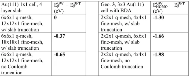
Table S1: Comparison of results from different treatment of the 𝐪 → 0 limit for bare Au(111) system as well as in Geo. 3. For the Au(111) cell, we compare the difference
between GW Fermi level and DFT Fermi level, i.e. EFGW− EFDFT; for Geo. 3, we compare
the difference between GW HOMO level and DFT Fermi level, i.e. EHOMOGW − EFDFT. We
see that the change in the GW HOMO level for different treatments of the 𝐪 → 0 limit was completely due to a corresponding GW Fermi level shift in an equivalent treatment of the 𝐪 → 0 limit for the Au(111) slab. Different fine meshes are used to approach the 𝐪 → 0 limit. With no Coulomb truncation, an averaging procedure is done in a region of the Brillouin Zone near 𝐪 = 0. It is important to note that the reference Fermi level of the GW spectrum has to be carefully calibrated against the DFT Fermi level. Otherwise, a rigid shift of the whole spectrum might result in incorrect level alignment predictions.
Au(111) 1x1 cell, 4 layer slab EF GW− E FDFT (eV) Geo. 3, 3x3 Au(111)
cell with BDA EHOMO
GW − E FDFT (eV) 6x6x1 q-mesh, 12x12x1 fine-mesh, w/ slab truncation 0 2x2x1 q-mesh, 4x4x1 fine-mesh, w/ slab truncation -1.30 6x6x1 q-mesh, 18x18x1 fine-mesh, w/ slab truncation -0.37 2x2x1 q-mesh, 6x6x1 fine-mesh, w/ slab truncation -1.66 6x6x1 q-mesh, 12x12x1 fine-mesh, no Coulomb truncation -0.65 2x2x1 q-mesh, 4x4x1 fine-mesh, no Coulomb truncation -1.98
6
4) GW convergence of gas-phase molecular orbital levels
Figure S2: Molecules investigated in this work. BDA: BenzeneDiAmine; FBDA:
Fluorinated BenzeneDiAmine; BPDA: BiPhenylDiAmine; BP: BiPyridine; BT: BenzeneThiol; BDT: BenzeneDiThiol.
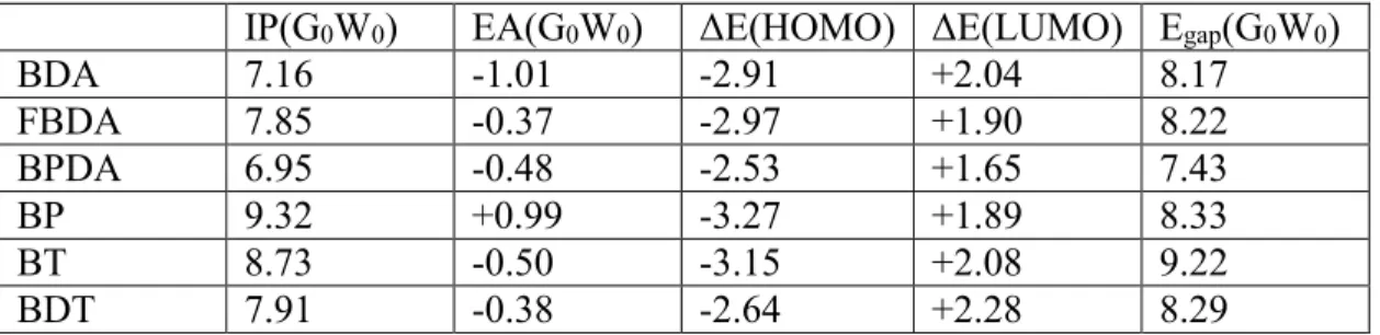
Table S2: Converged GW results for the studied gas-phase single molecules. ΔE’s refer
to GW correction upon their DFT corresponding levels. Egap = IP – EA. Energy units are
in eV. We note that the numbers reported here are obtained using a 24 Ry epsilon cutoff,
5000 bands for 15x15x15 Å3 cells (following previous literature [16]), and a box
Coulomb truncation scheme [9]. However, similar to Ref. [16], we obtain essentially the same results with a 20 Ry epsilon cutoff, which is used in our slab calculations.
IP(G0W0) EA(G0W0) ΔE(HOMO) ΔE(LUMO) Egap(G0W0)
BDA 7.16 -1.01 -2.91 +2.04 8.17 FBDA 7.85 -0.37 -2.97 +1.90 8.22 BPDA 6.95 -0.48 -2.53 +1.65 7.43 BP 9.32 +0.99 -3.27 +1.89 8.33 BT 8.73 -0.50 -3.15 +2.08 9.22 BDT 7.91 -0.38 -2.64 +2.28 8.29
5) Off-diagonal elements of GW self-energy evaluated in the BDA MO basis for Geometry 4
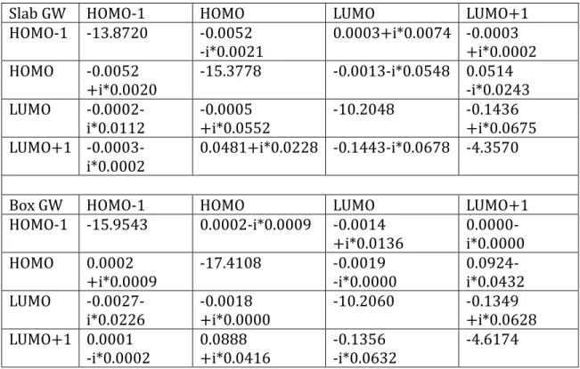
Table S3: Off-diagonal elements of GW self-energy evaluated in the BDA MO basis for
Geometry 4. Only MOs close to the frontier orbitals are considered, as orbitals further away have even smaller probability of mixing with the frontier MOs. Results are shown for both the slab and box truncation schemes. The self-energy for each entry is evaluated at the energy corresponding to the MO identified by the row index of the entry.
7
Slab GW HOMO-1 HOMO LUMO LUMO+1
HOMO-1 -13.8720 -0.0052 -i*0.0021 0.0003+i*0.0074 -0.0003 +i*0.0002 HOMO -0.0052 +i*0.0020 -15.3778 -0.0013-i*0.0548 0.0514 -i*0.0243 LUMO -0.0002-i*0.0112 -0.0005 +i*0.0552 -10.2048 -0.1436 +i*0.0675 LUMO+1 -0.0003-i*0.0002 0.0481+i*0.0228 -0.1443-i*0.0678 -4.3570
Box GW HOMO-1 HOMO LUMO LUMO+1
HOMO-1 -15.9543 0.0002-i*0.0009 -0.0014 +i*0.0136 0.0000-i*0.0000 HOMO 0.0002 +i*0.0009 -17.4108 -0.0019 -i*0.0000 0.0924-i*0.0432 LUMO -0.0027-i*0.0226 -0.0018 +i*0.0000 -10.2060 -0.1349 +i*0.0628 LUMO+1 0.0001 -i*0.0002 0.0888 +i*0.0416 -0.1356 -i*0.0632 -4.6174
6) Off-diagonal elements of GW self-energy evaluated in the BP MO basis for Geometry 7
Table S4: Off-diagonal elements of GW self-energy evaluated in the BP MO basis for
Geometry 7. Note that HOMO level at the interface is not well-defined here. Other details follow those in Table S3.
Slab GW HOMO-1 LUMO LUMO+1
HOMO-1 -17.7891 -0.0034-i*0.0095 0.0919-i*0.0428
LUMO -0.0032+i*0.0095 -13.7422 -0.0005-i*0.0041
LUMO+1 0.0922+i*0.0430 -0.0005+i*0.0041 -10.6064
Box GW HOMO-1 LUMO LUMO+1
HOMO-1 -20.0532 -0.0007+i*0.0001 0.0874-i*0.0409
LUMO -0.0007-i*0.0001 -16.0462 -0.0001+i*0.0001
8
7) Off-diagonal elements of GW self-energy evaluated in the BT MO basis for Geometry 11
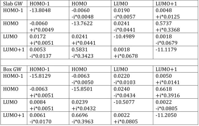
Table S5: Off-diagonal elements of GW self-energy evaluated in the BT MO basis for
Geometry 11. Note that HOMO level at the interface is not well-defined here. Other details follow those in Table S3.
Slab GW HOMO-1 HOMO LUMO LUMO+1
HOMO-1 -13.8048 -0.0060 -i*0.0048 0.0190 -i*0.0057 0.0048 +i*0.0125 HOMO -0.0060 +i*0.0049 -13.7622 0.0241 -i*0.0441 0.5737 +i*0.3368 LUMO 0.0172 +i*0.0051 0.0241 +i*0.0441 -10.4989 0.0018 -i*0.0679 LUMO+1 0.0053 -i*0.0137 0.5831 -i*0.3423 0.0018 +i*0.0678 -11.1179
Box GW HOMO-1 HOMO LUMO LUMO+1
HOMO-1 -15.8129 -0.0063 -i*0.0050 0.0220 -i*0.0103 0.0050 +i*0.0141 HOMO -0.0063 +i*0.0051 -15.8501 0.0240 -i*0.0434 0.6618 +i*0.3916 LUMO 0.0084 +i*0.0051 0.0239 +i*0.0432 -10.5077 0.0022 -i*0.0805 LUMO+1 0.0061 -i*0.0170 0.6696 -i*0.3963 0.0022 +i*0.0805 -11.2050
8) Other geometries considered for BDA molecular layer on Au(111)
The geometry used in Reference [6] was a face-on configuration in a 4x4 Au(111) cell, relaxed using DFT PBE without including van der Waals interactions. We have
performed a geometry optimization of the same system using the vdW-DF2 functional and found that this coverage is likely to be too low (Figure S3). Geometry optimization using the vdW-DF2 functional found that the benzene ring is tilted 18.2° from the surface. Similar geometry optimization for the 3x3 Au(111) cell found a corresponding
tilt angle of 24°, which is closer to the experimentally determined angle of 24°10°. We
also see that the amine group further from the surface is tilted toward the surface, away from the plane of the phenyl ring, by about 8°. This suggests that lower coverages would result in smaller tilt angles further from the experimental value, which is defined for “monolayer coverage” [6].
9
The geometry used in Reference [7] was a linear chain motif of BDA molecules on Au(111), which was experimentally observed at low temperature [17]. Using this same structure, we found a GW HOMO level of -0.75 eV and a DFT+Σ HOMO level of -2.58 eV (including the 0.3 eV intra-layer polarization as in Ref. [7]). The fact that GW
predicts a HOMO level much closer to EF than the UPS value indicates that the linear
chain geometry, which is stabilized by hydrogen bonds at 5 K [17], is not an appropriate geometry for the room temperature UPS experiment [6].
Figure S3. Optimized geometry of BDA in a 4x4 Au(111) cell in the face-on geometry
(VASP, vdW-DF2 functional).
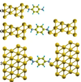
9) Geometries of metal/molecule/metal junction structures
Figure S4. a) BDA vertical up-right geometry in √3x√3 R30° Au(111) cell; b) Au(111) /BDA/Au(111) junction structure with √3x√3 R30° cell; c) Au(111)/BDA/Au(111) junction structure with 3x3cell.
10
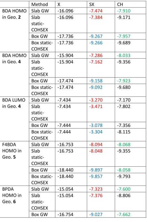
10) Decomposed self-energy contributions of MO levels from GW versus static-COHSEX results: Comprehensive result
Table S6: Components of the GW and static COHSEX self-energy corrections for
different geometries, together with the bare exchange term (X). SX is screened exchange, CH the Coulomb hole term. The GW self-energy is equal to difference between (SX+CH) and the mean-field exchange-correlation term. The X term is given for comparison. Units are in eV. The red, blue and green colors are used as a guide to the eye for the discussion in the main text.
Method X SX CH BDA HOMO in Geo. 2 Slab GW -16.096 -7.474 -7.910 Slab static-COHSEX -16.096 -7.384 -9.171 Box GW -17.736 -9.267 -7.957 Box static-COHSEX -17.736 -9.266 -9.689 BDA HOMO in Geo. 4 Slab GW -15.904 -7.286 -8.033 Slab static-COHSEX -15.904 -7.162 -9.356 Box GW -17.474 -9.158 -7.923 Box static-COHSEX -17.474 -9.092 -9.680 BDA LUMO in Geo. 4 Slab GW -7.434 -3.270 -7.170 Slab static-COHSEX -7.434 -3.471 -7.802 Box GW -7.444 -3.078 -7.356 Box static-COHSEX -7.444 -3.304 -8.115 F4BDA HOMO in Geo. 5 Slab GW -16.753 -8.094 -8.068 Slab static-COHSEX -16.753 -8.048 -9.355 Box GW -18.440 -9.897 -8.058 Box static-COHSEX -18.440 -9.857 -9.793 BPDA HOMO in Geo. 6 Slab GW -15.054 -7.323 -7.600 Slab static-COHSEX -15.054 -7.376 -8.806 Box GW -16.754 -9.027 -7.662
11 Box static-COHSEX -16.754 -9.041 -9.373 BP HOMO-1 in Geo. 7 Slab GW -20.019 -9.647 -7.976 Slab static-COHSEX -20.019 -9.543 -9.488 Box GW -21.603 -11.624 -7.878 Box static-COHSEX -21.603 -11.597 -9.846 BP LUMO in Geo. 7 Slab GW -13.810 -5.388 -8.388 Slab static-COHSEX -13.810 -5.200 -9.548 Box GW -9.677 -3.990 -8.500 Box static-COHSEX -9.677 -4.221 -9.438 BT HOMO in Geo. 8 Slab GW -13.877 -5.365 -8.159 Slab static-COHSEX -13.877 -4.960 -9.566 Box GW -15.105 -7.214 -7.813 Box static-COHSEX -15.105 -6.898 -9.564 BT HOMO in Geo. 9 Slab GW -13.652 -4.475 -8.536 Slab static-COHSEX -13.652 -4.089 -9.921 Box GW -15.451 -7.621 -7.594 Box static-COHSEX -15.451 -7.534 -9.301 BT LUMO in Geo. 9 Slab GW -7.422 -3.177 -7.730 Slab static-COHSEX -7.422 -3.408 -8.518 Box GW -7.448 -3.061 -7.538 Box static-COHSEX -7.448 -3.323 -8.297
12
11) Charge rearrangement and binding energy upon molecular adsorption on the Au(111) surface
Table S7: Number of electrons lost by the molecule (mol.) or the anchoring atom (N for
amine and pyridine, S for thiol), and binding energy upon adsorption of the molecule on the Au(111) surface. The desorbed hydrogen atom from thiol is taken to carry a charge of 1 electron, and is taken into consideration in the final result below. (Geo.: Geometry) There is little net charge transfer from the molecule to the metal, but for thiols, there is significant local charge rearrangement in the molecule. The binding energy is computed as the difference in energy between the hybrid system and the sum of the energies of the gas phase molecule/radical and the Au surface.
Geo.1 Geo.2 Geo.3 Geo.4 Geo.5 Geo.6 Geo.7 Geo.8 Geo.9 Geo.10 Mol. 0.086 0.182 0.159 0.193 0.142 0.177 0.048 -0.117 -0.167 -0.132 Anchor -0.019 -0.449 -0.385 0.144 0.106 0.117 0.158 -1.307 -1.411 -1.457 Binding energy (eV) -0.772 -1.502 -1.615 -1.083 -0.902 -1.023 -1.099 -2.217 -1.036 -0.999
Geo.4 @6L Au Geo.4 @4x4 Au Geo.9 @6L Au Geo.10 @6L Au Geo. 11
Mol. 0.197 0.227 -0.152 -0.107 -0.078 Anchor 0.129 0.159 -1.484 -1.442 -1.334 Binding energy (eV) -1.091 -1.123 - - -2.189
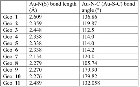
12) Molecule/metal slab geometric parameters
Table S8: Summary of geometric parameters for Geometries 1 to 11
Au-N(S) bond length (Å)
Au-N-C (Au-S-C) bond angle (°) Geo. 1 2.609 136.86 Geo. 2 2.359 119.87 Geo. 3 2.448 112.5 Geo. 4 2.338 114.0 Geo. 5 2.338 114.0 Geo. 6 2.338 114.2 Geo. 7 2.154 120.0 Geo. 8 2.279 105.74 Geo. 9 2.270 179.90 Geo. 10 2.276 179.82 Geo. 11 2.489 132.058
13
Atomic geometric coordinates of BDA/Au systems from Geo. 1 to Geo. 4 are also listed below. Coordinates for Geo. 5 ~ 11 are listed at the end of this document after the Reference section.
XYZ format coordinates for Geo. 1: 28 BDA/Au111 geo. 1 C 3.140518 1.457933 10.954336 C 4.460963 1.453559 13.472880 C 4.142933 2.650504 12.819166 C 3.523252 0.261119 11.567874 C 3.525667 2.652449 11.570825 C 4.140521 0.258851 12.816215 H 4.389917 3.604348 13.289313 H 3.274155 -0.689438 11.092153 H 3.278212 3.604650 11.097572 H 4.385838 -0.696546 13.284024 H 1.793448 2.298496 9.648112 H 5.549743 0.610949 14.995625 H 1.786475 0.626477 9.649273 H 5.551583 2.289944 14.997831 N 2.363610 1.460196 9.778419 N 5.026047 1.451323 14.757731 Au 0.240047 -0.004960 7.177793 Au 2.802509 1.455866 7.206997 Au 5.283109 2.917041 7.177696 Au 1.808581 0.009923 4.762676 Au 1.808580 2.901915 4.762701 Au 4.312146 1.455923 4.762151 Au 0.840531 1.455842 2.366993
14 Au 3.362124 0.000000 2.366993 Au 3.362124 2.911685 2.366993 Au 0.000000 0.000000 0.000000 Au 2.521593 1.455842 0.000000 Au 5.043187 2.911685 0.000000
XYZ format coordinates for Geo. 2:
================================================ 52 BDA/Au111 Geo. 2 C 4.761413451 4.019274501 10.522261754 C 2.620895606 3.443966919 12.262450780 C 3.946629270 3.451639331 12.723128482 C 3.451380398 3.970882823 10.059268094 C 5.001791441 3.737030845 11.864924817 C 2.393848463 3.694654121 10.902427675 H 4.148516089 3.250588215 13.771324166 H 3.257517136 4.149955505 9.004022563 H 6.017168085 3.762421231 12.252915793 H 1.388867942 3.658540452 10.489816377 H 6.733942585 4.147050554 9.981433813 H 0.692925395 2.941910612 12.718771470 H 5.803247145 5.361520897 9.365644656 H 1.772841755 2.788861356 14.005180670 N 5.812986221 4.366152204 9.611924720 N 1.561194696 3.246078170 13.131982881 Au 0.964117351 -0.348343041 7.742372139 Au 4.530236087 1.030773970 7.687033493
15 Au 7.141760993 0.161546092 7.333429351 Au 2.061175236 2.157113304 7.524095839 Au 5.767629850 3.550809856 7.398783007 Au 8.365987446 2.611175034 7.352368745 Au 3.766769803 5.469249307 7.103858434 Au 7.871989956 6.345623619 7.378606960 Au 10.100949264 4.767738419 7.051396140 Au 0.628253963 1.975131362 4.857349387 Au 4.359172220 1.190983249 5.010798781 Au 6.740363878 2.519484037 4.977290905 Au 2.860036358 3.546187156 5.119587743 Au 5.298448399 4.889206840 4.896292938 Au 8.182069279 4.993620986 4.899221627 Au 3.838905079 7.338305521 4.851147983 Au 6.682169373 7.428123119 4.979732177 Au 10.318582343 6.681125101 5.036800014 Au 1.507965000 0.870624000 2.462496000 Au 4.523894000 0.870624000 2.462496000 Au 7.539824000 0.870624000 2.462496000 Au 3.015929000 3.482495000 2.462496000 Au 6.031859000 3.482495000 2.462496000 Au 9.047789000 3.482495000 2.462496000 Au 4.523894000 6.094367000 2.462496000 Au 7.539824000 6.094367000 2.462496000 Au 10.555753000 6.094367000 2.462496000 Au 0.000000000 0.000000000 0.000000000 Au 3.015929000 0.000000000 0.000000000 Au 6.031859000 0.000000000 0.000000000
16 Au 1.507965000 2.611871000 0.000000000 Au 4.523894000 2.611871000 0.000000000 Au 7.539824000 2.611871000 0.000000000 Au 3.015929000 5.223743000 0.000000000 Au 6.031859000 5.223743000 0.000000000 Au 9.047789000 5.223743000 0.000000000
XYZ format coordinates for Geo. 3:
================================================ 52 BDA/Au111 Geo. 3 C 2.730355 2.522484 10.070164 C 5.422029 2.522759 10.925045 C 4.735766 3.730650 10.704206 C 3.410923 1.314465 10.276190 C 3.409572 3.730663 10.279437 C 4.737030 1.314724 10.700964 H 5.252808 4.683311 10.855477 H 2.903116 0.363397 10.082341 H 2.900752 4.681685 10.088120 H 5.255090 0.362164 10.849473 H 0.874735 3.363748 9.711786 H 7.264235 1.673163 11.253534 H 0.875384 1.680238 9.712041 H 7.263835 3.372660 11.255507 N 1.420943 2.522159 9.519558 N 6.728310 2.522613 11.407515 Au -0.011328 -0.021809 7.093648 Au 1.432353 2.519782 7.071760 Au 2.916514 5.057871 7.063904 Au 2.914489 -0.022022 7.066985 Au 4.382766 2.519448 7.050173 Au 5.824010 5.041463 7.104085 Au 5.822985 -0.003273 7.101907 Au 7.253042 2.521951 7.093094 Au 8.720242 5.058489 7.096251 Au -1.460520 -0.835989 4.700900 Au -0.003236 1.679730 4.724558 Au 1.449835 4.198133 4.724686
17 Au 1.450752 -0.844558 4.710308 Au 2.901150 1.682475 4.725055 Au 4.369957 4.207025 4.706791 Au 4.371940 -0.840565 4.703816 Au 5.826000 1.672797 4.702075 Au 7.277906 4.202270 4.714493 Au 10.190898 5.883718 2.366993 Au 7.279213 0.840531 2.366993 Au 8.735055 3.362125 2.366993 Au 4.367527 5.883718 2.366993 Au 1.455842 0.840531 2.366993 Au 2.911685 3.362125 2.366993 Au 7.279212 5.883718 2.366993 Au 4.367527 0.840531 2.366993 Au 5.823370 3.362125 2.366993 Au 0.000000 0.000000 0.000000 Au 1.455843 2.521594 0.000000 Au 2.911685 5.043188 0.000000 Au 2.911685 0.000000 0.000000 Au 4.367527 2.521594 0.000000 Au 5.823370 5.043188 0.000000 Au 5.823370 0.000000 0.000000 Au 7.279213 2.521594 0.000000 Au 8.735055 5.043188 0.000000
XYZ format coordinates for Geo. 4:
================================================ 53 BDA/Au111 Geo.4 C 1.891566814 4.576038109 11.573503922 C 1.832116814 4.543150409 14.408967922 C 2.442723814 3.513916254 13.685161622 C 1.274174814 5.601394909 12.297214522 C 2.470823814 3.528774977 12.297576922 C 1.245677014 5.585894609 13.684983222 H 2.905559814 2.687522649 14.219049422 H 0.803113014 6.424243409 11.765379422 H 2.947296814 2.707463029 11.768434522 H 0.763359114 6.403440209 14.215219522 H 2.598312814 4.012539629 9.744261222 H 1.123661014 5.089952909 16.242661122 H 1.782871814 5.467323309 9.739604922
18 H 1.956700814 3.648590329 16.235336122 N 1.866445814 4.560087409 10.173820022 N 1.866410814 4.560116309 15.809484122 Au 0.000000604 3.482494306 9.268659967 Au 0.000000000 0.000000000 7.201817163 Au -1.507964117 2.611870469 7.201817163 Au -3.015928234 5.223740938 7.201817163 Au 3.015928239 0.000000000 7.201817163 Au 1.507964122 2.611870469 7.201817163 Au 0.000000005 5.223740938 7.201817163 Au 6.031856478 0.000000000 7.201817163 Au 4.523892361 2.611870469 7.201817163 Au 3.015928244 5.223740938 7.201817163 Au 0.000000000 1.741247675 4.842043812 Au -1.507964117 4.353118144 4.842043812 Au -3.015928234 6.964988613 4.842043812 Au 3.015928239 1.741247675 4.842043812 Au 1.507964122 4.353118144 4.842043812 Au 0.000000005 6.964988613 4.842043812 Au 6.031856478 1.741247675 4.842043812 Au 4.523892361 4.353118144 4.842043812 Au 3.015928244 6.964988613 4.842043812 Au 1.507964721 0.870623837 2.462496078 Au 0.000000604 3.482494306 2.462496078 Au -1.507963513 6.094364775 2.462496078 Au 4.523892960 0.870623837 2.462496078 Au 3.015928843 3.482494306 2.462496078 Au 1.507964726 6.094364775 2.462496078 Au 7.539821199 0.870623837 2.462496078 Au 6.031857082 3.482494306 2.462496078 Au 4.523892965 6.094364775 2.462496078 Au 0.000000000 0.000000000 0.000000000 Au -1.507964117 2.611870469 0.000000000 Au -3.015928234 5.223740938 0.000000000 Au 3.015928239 0.000000000 0.000000000 Au 1.507964122 2.611870469 0.000000000 Au 0.000000005 5.223740938 0.000000000 Au 6.031856478 0.000000000 0.000000000 Au 4.523892361 2.611870469 0.000000000 Au 3.015928244 5.223740938 0.000000000
19
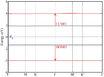
13) DFT and GW bandstructure for the BDA layer as in Geo. 4
Figure S5. DFT (Black) and GW (Red) bandstructure for BDA molecular layer as in
Geo. 4, along the k-path Γ → M → K → Γ → M′ → K′ → Γ calculated with 4x4 k-mesh sampling, and 12 Ry epsilon cutoff in GW calculation. Bandwidth for HOMO and LUMO bands are 0.00055 eV (0.00066 eV) and 0.025 eV (0.073 eV) respectively, for the DFT (GW) results. They are not dispersive across the Brillouin zone. GW HOMO-LUMO gap at Γ for the layer is 7.959 eV, while the corresponding Wigner-Seitz truncation gives 8.169 eV. So the intra-molecular layer polarization effect is only 0.21 eV.
14) GW projected molecular level dispersion across the Brillouin zone
We also performed slab truncation GW projection calculations of the HOMO and LUMO levels of BDA as in Geo. 4 at another three k-points in the Brillouin zone (BZ). The results are summarized in the table below (with respect to the Fermi level). There is seen to be little dispersion even for the projected levels from the molecule-metal hybrid slab. This indicates the molecular band gap renormalization we observe is not from BZ dispersion of the adsorbed molecular layer. A molecular layer GW projected bandstructure is currently beyond the reach of our computational capabilities.
Table S9 Slab GW HOMO and LUMO levels for Geometry 4
(eV) Γ K=(0.0, 0.5, 0.0) K=(0.5, 0.0, 0.0) K=(0.5, 0.5, 0.0) HOMO -1.344 -1.345 -1.345 -1.346 LUMO +4.230 +4.208 +4.207 +4.251
20
15) Calculated image charge correction energy for the hybridized slabs Table S10: Image charge model correction energy for various MO levels in the
hybridized geometries investigated in this work. Here, we compare the image charge correction we have computed with that assuming a unit of point charge (point charge method) at the ring center or in the middle of the molecule (Geometries 6 and 7 where there are two rings). The image plane is taken to be 0.9 Å above the Au(111) surface.
Geo.1 HOMO Geo.2 HOMO Geo.3 HOMO Geo. 4 HOMO Geo.5 HOMO Geo.6 HOMO Image charge
correction used in the main text (eV)
0.9612 1.2181 1.3059 0.8174 0.8129 0.5913
Distance of point charge from image plane (Å)
4.126 3.094 2.515 4.889 4.892 7.043
Point charge method (eV) 0.8725 1.1630 1.4314 0.7363 0.7358 0.5112 Geo.7 LUMO Geo.8 HOMO Geo.9 HOMO Geo.10 HOMO Geo.11 HOMO Image charge
correction used in the main text (eV)
0.5631 0.8639 0.7729 0.5937 2.3382
Distance of point charge from image plane (Å)
6.864 5.447 6.590 6.576 3.957
Point charge method (eV)
0.5239 0.6609 0.5463 0.5474 0.9097
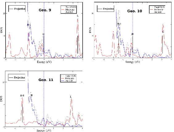
16) Projected density of states together with our DFT starting points marked for Geo.’s 1-11 investigated in this work.
22
Figure S6. Projected density of states plots, with our wavefunction based projected
DFT HOMO-1 (H-1), HOMO (H), LUMO (L), and LUMO+1 (L+1) starting point levels marked on the same plot.
17) Table S11 is given in the next page.
23 1 17 ) S umma ry o f e ne rg y le ve ls o f g eo me tr ie s i nv es tig ate d in th is w or k. 2 Ta bl e S1 1: E ne rg y le ve ls fo r v ar io us str uc tu re s. F er mi le ve ls a re a bs ol ute v al ue s f or e ac h ca lc ul ati on , w hi le a ll th e re st da ta a re g iv en w ith re sp ec tiv e to th e mo le cu le /me ta l s la b Fe rmi le ve l o f e ac h ca se . 3 Sy ste m DF T HO M O GW H O M O (S la b) GW H O M O (B ox ) Ima ge M eth H O M O DF T LU M O GW LU M O (S la b) GW LU M O (B ox ) Ima ge M eth LU M O E_ Fe rmi 4 BD A-Tl /3 x3 Au 11 1 N oA d PB E-D2 (2 ) -0 .8 73 -1 .3 39 2 -3 .1 81 -2 .5 69 8 3. 03 64 3. 70 04 3. 53 94 3. 87 48 3. 83 52 5 BD A-Tl /3 x3 Au 11 1 W /A d PB E-D2 -0 .2 85 2 -0 .7 42 6 -2 .6 01 2 -2 .2 21 2. 96 02 3. 35 3. 21 52 4. 09 93 4. 04 91 6 BD A-Tl /S qr (3 )^ 2 R3 0 Au N oA d Vd W (1 ) -1 .1 72 6 -1 .6 42 8 -4 .2 11 2 -3 .1 25 4 2. 07 44 2. 78 94 N on e 3. 25 01 5. 28 74 7 BD A-Tl /S qr (3 )^ 2 R3 0 Au W /A d Vd W -2 .5 63 4 -3 .4 12 3 -5 .5 62 3 -4 .8 10 4 0. 61 9 W rg O cc . N on e 2. 03 05 6. 63 85 8 BD A-Fa ce /3 x3 Au 11 1 N oA d Vd W (3 ) -0 .9 9 -1 .2 98 8 N on e -2 .5 98 1 N .A . N .A . N on e N on e 5. 96 61 9 BD A-Fa ce /3 x3 Au 11 1 W /A d Q E -1 .6 53 -2 .2 55 9 N on e -3 .8 02 5 1. 86 43 2. 68 49 N on e 3. 13 77 4. 34 14 10 BD A-Fa ce /3 x3 Au 11 1 N oA d Q E -0 .8 71 2 -1 .1 77 9 N on e -2 .5 15 5 N .A . N .A . N on e N on e 4. 76 46 11 BD A-Ve rt/ 3x 3A u1 11 W /A d Q E (4 ) -0 .9 58 2 -1 .3 44 3 -3 .1 07 4 -3 .0 54 8 2. 51 57 4. 23 03 4. 23 6 3. 82 22 3. 61 68 12 Ib id (S ta t.-COH SE X) -0 .9 58 2 -2 .5 42 8 -4 .7 96 6 as a bo ve 2. 51 57 3. 39 67 3. 25 04 as a bo ve ib id 13 BD A-Ve rt/ 3x 3A u1 11 W /A d Vd W -1 .0 59 -1 .4 88 3 -3 .3 57 5 n. a. 2. 82 43 2. 89 19 2. 52 05 n. a. 4. 27 37 14 BD A-Li nCh ai n/ Au 11 1 N oA d @ G. Li -0 .5 71 -0 .7 50 1 N on e N .A . 2. 93 74 4. 20 39 N on e N .A . 4. 20 96 15 F4 BD A-Ve rt/ 3x 3A u1 11 w /A d Vd W (5 ) -1 .1 80 4 -1 .7 12 8 -3 .5 07 4 -3 .3 34 5 2. 49 34 3. 58 88 3. 33 88 3. 66 2 4. 33 61 16 BP DA -V er t/ 3x 3A u1 11 w /A d Vd W (6 ) -0 .7 64 9 -1 .1 67 2 -2 .9 35 6 -2 .7 02 6 2. 57 65 3. 66 86 3. 33 8 3. 66 84 3. 52 2 17 Bp yd -V er t/ 3x 3A u1 11 w /A d Vd W (7 ) N .A . N .A . N .A . N .A . 0. 17 82 0. 39 92 1. 68 56 1. 50 81 4. 02 53 18 Ib id (S ta t.-COH SE X) N .A . N .A . N .A . as a bo ve 0. 17 82 W rg O cc 0. 51 58 as a bo ve ib id 19 BD A-Ve rt/ 4x 4A u1 11 4 L W /A d Vd W (4 '') -0 .5 85 6 N .A . -2 .3 74 9 -2 .6 82 2 2. 80 16 N .A . 4. 21 29 4. 10 81 3. 01 78 20 BD A-Ve rt/ 3x 3A u1 11 6 L W /A d Vd W (4 ') -0 .8 05 2 N .A . -2 .7 75 9 -2 .9 01 8 2. 62 82 N .A . 4. 23 18 3. 93 47 5. 44 39 21 BD A-Ve rt/ Sq r( 3) ^2 R 30 W / A d Vd W -1 .1 38 1 -1 .7 85 3 -4 .4 26 6 -3 .2 35 8 1. 59 64 W rg O cc . W rg O cc . 2. 90 32 6. 01 06 22 Au /B DA -V t/ Au S qr (3 )^ 2 R3 0 Ad Ju nc -1 .2 14 2 -1 .4 84 -4 .0 57 9 -2 .9 53 2 1. 29 77 W rg O cc . W rg O cc . 2. 29 47 9. 67 87 23 Au /B DA -V t/ Au 3 x3 A d Ju nc -0 .5 85 5 N on e -2 .1 46 -2 .3 21 2 2. 64 48 N on e 4. 00 31 3. 64 1 6. 52 64 24 Au /B P-Vt/ Au 3 x3 A d Ju nc N .A . N .A . N .A . N .A . 0. 38 79 N on e 0. 83 86 1. 48 85 6. 56 12 25 BD A/ Sq r( 3) ^2 R 30 N oA d PB E-D2 (1 ') -1 .0 87 -1 .6 98 4 N on e -3 2. 36 67 2. 99 18 N on e 3. 46 84 4. 27 09 26 BT /S qr (3 )^ 2 R3 0 W /A d PB E-D2 -0 .3 71 6 -1 .0 26 1 N on e -2 .2 32 7 2. 64 72 3. 66 02 N on e 3. 95 6 4. 55 05 27 BT -T l/ 3x 3A u1 11 4 L w /A d Vd W (8 ) -0 .2 73 -0 .7 21 2 -2 .2 25 2 -2 .5 55 1 3. 45 41 4. 83 32 4. 80 44 4. 87 34 3. 45 17 28 Ib id (S ta t.-COH SE X) -0 .2 73 -1 .7 23 2 -3 .6 59 4 as a bo ve 3. 45 41 3. 87 39 3. 76 52 as a bo ve ib id 29 BT -R lx /3 x3 Au 11 1 4L N oA d Vd W (1 1) -1 .2 63 9 -1 .8 04 8 -3 .5 96 8 -2 .0 71 7 2. 82 52 4. 45 58 4. 44 92 3. 99 09 3. 69 74 30 Ib id (S ta t.-COH SE X) -1 .2 63 9 -2 .9 64 2 -5 .2 78 7 as a bo ve 2. 82 52 3. 49 46 3. 40 63 as a bo ve ib id 31 BT -R lx /3 x3 Au 11 1 4L w /A d Vd W (9 ) -0 .0 36 2 -0 .2 71 1 -2 .4 78 6 -2 .4 09 3 3. 49 58 4. 89 48 5. 20 38 5. 02 71 3. 41 69 32 Ib id (S ta t.-COH SE X) -0 .0 36 2 -1 .2 70 5 -4 .0 96 as a bo ve 3. 49 58 3. 87 63 4. 18 18 as a bo ve ib id 33 BT -R lx /3 x3 Au 11 1 6L A d Vd W -0 .1 58 6 N on e -2 .1 5 -2 .5 31 7 3. 42 57 N on e 4. 92 31 4. 95 7 5. 23 95 34 BD T-Ve rt/ 3x 3A u1 11 4 L W /A d Vd W (1 0) -0 .0 04 4 -0 .3 44 4 -2 .5 53 2 -2 .0 55 7 3. 1 4. 39 67 4. 74 1 4. 83 25 3. 61 24 35 BD T-Ve rt/ 3x 3A u1 11 6 L W /A d Vd W -0 .1 12 7 N on e -2 .2 74 6 -2 .1 64 3. 03 27 N on e 4. 46 43 4. 76 52 5. 41 4
24 References
[1] G. Kresse and J. Furthmuller, Computational Materials Science 6, 15 (1996).
[2] P. Giannozzi et al., Journal of Physics-Condensed Matter 21, 19, 395502 (2009).
[3] S. Grimme, Journal of Computational Chemistry 27, 1787 (2006).
[4] M. Dion, H. Rydberg, E. Schroder, D. C. Langreth, and B. I. Lundqvist, Physical
Review Letters 92, 4, 246401 (2004).
[5] J. Klimes, D. R. Bowler, and A. Michaelides, Physical Review B 83, 195131 (2011).
[6] M. Dell'Angela et al., Nano Letters 10, 2470 (2010).
[7] G. Li, T. Rangel, Z.-F. Liu, V. R. Cooper, and J. B. Neaton, Physical Review B 93,
125429 (2016).
[8] G. Henkelman, A. Arnaldsson, and H. Jonsson, Computational Materials Science
36, 354 (2006).
[9] J. Deslippe, G. Samsonidze, D. A. Strubbe, M. Jain, M. L. Cohen, and S. G. Louie,
Computer Physics Communications 183, 1269 (2012).
[10] T. Rangel, D. Kecik, P. E. Trevisanutto, G. M. Rignanese, H. Van Swygenhoven,
and V. Olevano, Physical Review B 86, 125125 (2012).
[11] J. Deslippe, G. Samsonidze, M. Jain, M. L. Cohen, and S. G. Louie, Physical Review
B 87, 165124 (2013).
[12] Y. J. Zheng et al., Acs Nano 10, 2476 (2016).
[13] D. A. Egger, Z. F. Liu, J. B. Neaton, and L. Kronik, Nano Letters 15, 2448 (2015).
[14] J. M. Soler, E. Artacho, J. D. Gale, A. Garcia, J. Junquera, P. Ordejon, and D.
Sanchez-Portal, Journal of Physics-Condensed Matter 14, 2745, Pii s0953-8984(02)30737-9 (2002).
[15] A. Kokalj, Computational Materials Science 28, 155 (2003).
[16] S. Sharifzadeh, I. Tamblyn, P. Doak, P. T. Darancet, and J. B. Neaton, European
Physical Journal B 85, 323 (2012).
[17] T. K. Haxton, H. Zhou, I. Tamblyn, D. Eom, Z. H. Hu, J. B. Neaton, T. F. Heinz, and
S. Whitelam, Physical Review Letters 111, 5, 265701 (2013).
XYZ format coordinates for Geo. 5:
================================================ 53 FBDA/Au111 Geo.5 C 3.346936459 1.933185327 11.504639189 C 3.284275559 1.898938327 14.371124289 C 3.891758959 0.882371327 13.631277989 C 2.740061959 2.950213427 12.244251689 C 3.922006159 0.899107327 12.245656989 C 2.709002959 2.933199927 13.630192789
25 F 4.466391559 -0.144357673 14.304729489 F 2.174253959 3.981608427 11.570697789 F 4.529808959 -0.109429673 11.573615989 F 2.107283159 3.945006327 14.302213689 H 4.046689959 1.358908327 9.690505489 H 2.583575959 2.465780227 16.188327589 H 3.217785559 2.825453727 9.687817089 H 3.428218359 1.008035327 16.187054589 N 3.322287359 1.918124327 10.117536089 N 3.310993659 1.914196327 15.758096589 Au 1.455842 0.840531 9.212376 Au 0.000000 0.000000 7.145576 Au 1.455842 2.521594 7.145576 Au 2.911685 5.043187 7.145576 Au 2.911685 0.000000 7.145576 Au 4.367527 2.521594 7.145576 Au 5.823370 5.043187 7.145576 Au 5.823370 0.000000 7.145576 Au 7.279213 2.521594 7.145576 Au 8.735055 5.043187 7.145576 Au -1.455842 -0.840530 4.740462 Au 0.000000 1.681062 4.740462 Au 1.455842 4.202656 4.740462 Au 1.455842 -0.840530 4.740462 Au 2.911685 1.681062 4.740462 Au 4.367527 4.202656 4.740462 Au 4.367527 -0.840530 4.740462 Au 5.823370 1.681062 4.740462 Au 7.279212 4.202656 4.740462 Au -2.911684 -1.681061 2.366993 Au -1.455842 0.840531 2.366993 Au 0.000000 3.362125 2.366993 Au 0.000000 -1.681061 2.366993 Au 1.455842 0.840531 2.366993 Au 2.911685 3.362125 2.366993 Au 2.911685 -1.681061 2.366993 Au 4.367527 0.840531 2.366993 Au 5.823370 3.362125 2.366993 Au 0.000000 0.000000 0.000000 Au 1.455842 2.521594 0.000000 Au 2.911685 5.043187 0.000000 Au 2.911685 0.000000 0.000000 Au 4.367527 2.521594 0.000000 Au 5.823370 5.043187 0.000000 Au 5.823370 0.000000 0.000000
26 Au 7.279213 2.521594 0.000000 Au 8.735055 5.043187 0.000000
XYZ format coordinates for Geo. 6:
================================================ 63 BPDA/Au111 Geo. 6 C 3.355147993 1.929198734 11.507437954 C 3.335166093 1.898626734 15.824901554 C 2.746321293 2.959346734 12.235939054 C 2.251890783 2.406469734 16.555333154 C 2.744683193 2.943040834 13.621835254 C 2.236940743 2.406404734 17.941023154 C 3.340460893 1.904830734 14.351695054 C 3.315899293 1.887271734 18.669003154 C 3.937884493 0.875307734 13.611186954 C 4.408231393 1.382604734 17.951214154 C 3.946577693 0.880544734 12.224902154 C 4.411557793 1.389212734 16.565165554 H 2.279821273 3.786867134 11.705902554 H 1.383887413 2.786858534 16.024913754 H 2.291950583 3.775274234 14.152350454 H 1.373523833 2.802698134 18.470975154 H 4.387785293 0.035310734 14.132204554 H 5.269483193 0.994900734 18.490933154 H 4.405103293 0.055064734 11.685146354 H 5.285158793 1.009420734 16.043815654 H 4.025957493 1.359131734 9.659574754 H 3.180130793 2.809911734 9.668415554 H 2.427767873 1.997757734 20.508727154 H 3.940838193 1.269188734 20.517403154 N 3.322287393 1.918023734 10.117536054 N 3.327639693 1.925412734 20.058623154 Au 1.455842 0.840531 9.212376 Au 0.000000 0.000000 7.145576 Au 1.455842 2.521594 7.145576 Au 2.911685 5.043187 7.145576 Au 2.911685 0.000000 7.145576 Au 4.367527 2.521594 7.145576 Au 5.823370 5.043187 7.145576 Au 5.823370 0.000000 7.145576 Au 7.279213 2.521594 7.145576 Au 8.735055 5.043187 7.145576 Au -1.455842 -0.840530 4.740462
27 Au 0.000000 1.681062 4.740462 Au 1.455842 4.202656 4.740462 Au 1.455842 -0.840530 4.740462 Au 2.911685 1.681062 4.740462 Au 4.367527 4.202656 4.740462 Au 4.367527 -0.840530 4.740462 Au 5.823370 1.681062 4.740462 Au 7.279212 4.202656 4.740462 Au -2.911684 -1.681061 2.366993 Au -1.455842 0.840531 2.366993 Au 0.000000 3.362125 2.366993 Au 0.000000 -1.681061 2.366993 Au 1.455842 0.840531 2.366993 Au 2.911685 3.362125 2.366993 Au 2.911685 -1.681061 2.366993 Au 4.367527 0.840531 2.366993 Au 5.823370 3.362125 2.366993 Au 0.000000 0.000000 0.000000 Au 1.455842 2.521594 0.000000 Au 2.911685 5.043187 0.000000 Au 2.911685 0.000000 0.000000 Au 4.367527 2.521594 0.000000 Au 5.823370 5.043187 0.000000 Au 5.823370 0.000000 0.000000 Au 7.279213 2.521594 0.000000 Au 8.735055 5.043187 0.000000
XYZ format coordinates for Geo. 7:
================================================ 57 BP/Au111 Geo. 7 C 2.609926793 0.821302516 12.056242343 C 0.448298316 0.339810507 17.767854339 C 2.649631142 0.833870231 13.435745220 C 0.393356000 0.323579453 16.379715619 C 1.460313362 0.842881731 14.176526920 C 1.464719776 0.842743837 15.643683747 C 0.266784301 0.848458909 13.442073723 C 2.540800797 1.358348077 16.375483503 C 0.298820733 0.845534869 12.062005361 C 2.492748462 1.338967827 17.763943210 H 3.516483889 0.798050830 11.459771484 H -0.371864948 -0.076305610 18.349660787
28 H 3.611368932 0.810875717 13.934398978 H -0.462652251 -0.117662284 15.879364189 H -0.691999414 0.878410069 13.946053359 H 3.395731724 1.798424833 15.872675457 H -0.611111453 0.864182907 11.470558529 H 3.315778389 1.752749059 18.343104391 N 1.452606489 0.827735032 11.365970727 N 1.471978177 0.839046221 18.467563258 Au 1.455842000 0.840531000 9.212376000 Au 0.000000000 0.000000000 7.145576000 Au 1.455842000 2.521594000 7.145576000 Au 2.911685000 5.043187000 7.145576000 Au 2.911685000 0.000000000 7.145576000 Au 4.367527000 2.521594000 7.145576000 Au 5.823370000 5.043187000 7.145576000 Au 5.823370000 0.000000000 7.145576000 Au 7.279213000 2.521594000 7.145576000 Au 8.735055000 5.043187000 7.145576000 Au -1.455842000 -0.840530000 4.740462000 Au -0.000000000 1.681062000 4.740462000 Au 1.455842000 4.202656000 4.740462000 Au 1.455842000 -0.840530000 4.740462000 Au 2.911685000 1.681062000 4.740462000 Au 4.367527000 4.202656000 4.740462000 Au 4.367527000 -0.840530000 4.740462000 Au 5.823370000 1.681062000 4.740462000 Au 7.279212000 4.202656000 4.740462000 Au -2.911684000 -1.681061000 2.366993000 Au -1.455842000 0.840531000 2.366993000 Au -0.000000000 3.362125000 2.366993000 Au -0.000000000 -1.681061000 2.366993000 Au 1.455842000 0.840531000 2.366993000 Au 2.911685000 3.362125000 2.366993000 Au 2.911685000 -1.681061000 2.366993000 Au 4.367527000 0.840531000 2.366993000 Au 5.823370000 3.362125000 2.366993000 Au 0.000000000 0.000000000 0.000000000 Au 1.455842000 2.521594000 0.000000000 Au 2.911685000 5.043187000 0.000000000 Au 2.911685000 0.000000000 0.000000000 Au 4.367527000 2.521594000 0.000000000 Au 5.823370000 5.043187000 0.000000000 Au 5.823370000 0.000000000 0.000000000 Au 7.279213000 2.521594000 0.000000000 Au 8.735055000 5.043187000 0.000000000
29
XYZ format coordinates for Geo. 8:
================================================ 49 BT/Au111 Geo. 8 C 2.150145 -1.230141 14.477068 C 3.115240 -0.239798 14.271947 C 1.018261 -1.278469 13.655580 C 1.811997 0.660244 12.432239 C 0.843390 -0.339825 12.640182 C 2.953773 0.698985 13.253397 H 2.279572 -1.963974 15.275338 H 4.003986 -0.199515 14.906179 H 0.260375 -2.050132 13.811606 H -0.046466 -0.365081 12.006510 H 3.709088 1.469532 13.082018 S 1.587966 1.944259 11.238962 Au 1.465806 0.896358 9.218989 Au -0.039413 -0.033752 7.150378 Au 1.458566 2.592555 7.053531 Au 2.911708 5.051297 7.108723 Au 2.941963 -0.020757 7.118739 Au 4.381521 2.531892 7.098454 Au 5.824805 5.037709 7.118122 Au 5.822330 0.004812 7.106397 Au 7.270741 2.529382 7.098300 Au 8.731442 5.053135 7.117217 Au -1.441147 -0.828900 4.739646 Au -0.001690 1.669536 4.742193 Au 1.451877 4.211063 4.714260 Au 1.449829 -0.831777 4.749635 Au 2.916351 1.681528 4.720239 Au 4.367039 4.207519 4.722154 Au 4.357423 -0.834021 4.729552 Au 5.823437 1.678444 4.717889 Au 7.281885 4.209522 4.722643 Au -2.911684 -1.681061 2.366993 Au -1.455842 0.840531 2.366993 Au 0.000000 3.362125 2.366993 Au 0.000000 -1.681061 2.366993 Au 1.455842 0.840531 2.366993 Au 2.911685 3.362125 2.366993 Au 2.911685 -1.681061 2.366993
30 Au 4.367527 0.840531 2.366993 Au 5.823370 3.362125 2.366993 Au 0.000000 0.000000 0.000000 Au 1.455843 2.521594 0.000000 Au 2.911685 5.043187 0.000000 Au 2.911685 0.000000 0.000000 Au 4.367527 2.521594 0.000000 Au 5.823370 5.043187 0.000000 Au 5.823370 0.000000 0.000000 Au 7.279213 2.521594 0.000000 Au 8.731442 5.053135 0.000000
XYZ format coordinates for Geo. 9:
================================================ 49 BT/Au111 Geo. 9 C 1.426690 0.839128 15.979084 C 1.437812 0.838811 13.179546 C 0.219173 0.838967 15.272281 C 0.214734 0.838797 13.879280 C 2.639688 0.838943 15.281778 C 2.655425 0.838801 13.888760 H -0.730831 0.838986 15.812101 H -0.722712 0.839139 13.320462 H 3.585295 0.838949 15.829356 H 3.597467 0.839153 13.337756 H 1.422346 0.839351 17.071012 S 1.442356 0.838610 11.425965 Au 1.450868 0.841494 9.156417 Au -0.052733 -0.034792 7.091561 Au 1.453200 2.582392 7.096040 Au 2.907229 5.041691 7.093721 Au 2.958261 -0.034232 7.093453 Au 4.375841 2.526106 7.080925 Au 5.820825 5.029961 7.083813 Au 5.820347 -0.002465 7.089806 Au 7.265927 2.526024 7.081017 Au 8.734023 5.042040 7.093887 Au 2.920018 6.727657 4.719918 Au 0.002202 1.677897 4.721198 Au 1.454337 4.189516 4.719575 Au 5.821989 6.724917 4.718755 Au 2.906571 1.677815 4.721424
31 Au 4.361479 4.203880 4.712465 Au 8.723205 6.727948 4.720487 Au 5.821971 1.673987 4.711652 Au 7.282404 4.203845 4.712494 Au 10.190896 5.883717 2.366993 Au 7.279211 0.840531 2.366993 Au 8.735053 3.362125 2.366993 Au 4.367527 5.883717 2.366993 Au 1.455842 0.840531 2.366993 Au 2.911685 3.362125 2.366993 Au 7.279212 5.883717 2.366993 Au 4.367527 0.840531 2.366993 Au 5.823370 3.362125 2.366993 Au 0.000000 0.000000 0.000000 Au 1.455843 2.521594 0.000000 Au 2.911685 5.043187 0.000000 Au 2.911685 0.000000 0.000000 Au 4.367527 2.521594 0.000000 Au 5.823370 5.043187 0.000000 Au 5.823370 0.000000 0.000000 Au 7.279213 2.521594 0.000000 Au 8.735055 5.043187 0.000000
XYZ format coordinates for Geo. 10:
================================================ 50 BDA/Au111 Geo. 10 C 1.450287 0.839070 15.967575 C 1.436239 0.839678 13.152452 C 0.232534 0.839533 15.261061 C 0.222492 0.839878 13.872808 C 2.660110 0.839449 15.250630 C 2.655280 0.839722 13.862775 H -0.714431 0.839709 15.807552 H -0.722960 0.840254 13.327235 H 3.613864 0.839714 15.784193 H 3.595005 0.840010 13.307438 H 2.714658 0.835950 17.932905 S 1.380408 0.838385 17.723131 S 1.441391 0.837451 11.411168 Au 1.441553 0.837765 9.135625 Au -0.057260 -0.039232 7.074550 Au 1.453108 2.584203 7.083807 Au 2.906261 5.039850 7.092668
32 Au 2.958892 -0.036463 7.080940 Au 4.376632 2.525972 7.079947 Au 5.820942 5.029329 7.083890 Au 5.818905 -0.002927 7.088006 Au 7.265678 2.525811 7.080161 Au 8.734281 5.041441 7.093029 Au 2.917288 6.725523 4.715117 Au 0.001077 1.678335 4.716452 Au 1.454314 4.190536 4.715515 Au 5.822172 6.722654 4.713393 Au 2.907832 1.678137 4.717274 Au 4.362059 4.203358 4.712223 Au 8.724665 6.726484 4.716837 Au 5.822145 1.674022 4.711135 Au 7.282074 4.203297 4.712359 Au 10.190896 5.883717 2.366993 Au 7.279211 0.840531 2.366993 Au 8.735053 3.362125 2.366993 Au 4.367527 5.883717 2.366993 Au 1.455842 0.840531 2.366993 Au 2.911685 3.362125 2.366993 Au 7.279212 5.883717 2.366993 Au 4.367527 0.840531 2.366993 Au 5.823370 3.362125 2.366993 Au 0.000000 0.000000 0.000000 Au 1.455843 2.521594 0.000000 Au 2.911685 5.043187 0.000000 Au 2.911685 0.000000 0.000000 Au 4.367527 2.521594 0.000000 Au 5.823370 5.043187 0.000000 Au 5.823370 0.000000 0.000000 Au 7.279213 2.521594 0.000000 Au 8.735055 5.043187 0.000000
XYZ format coordinates for Geo. 11:
================================================ 48 BT/Au111 Geo.11 C 1.427023 0.835287 13.362285 C 1.444150 0.813753 10.575703 C 0.220572 0.827981 12.655337 C 0.219814 0.816530 11.259890 C 2.642057 0.828828 12.670319
33 C 2.660004 0.817531 11.274996 H -0.729934 0.830400 13.194242 H -0.718246 0.809103 10.698633 H 3.585868 0.831860 13.220914 H 3.604888 0.810943 10.725375 H 1.420272 0.844064 14.454275 S 1.456048 0.832010 8.793631 Au -0.144635 -0.082733 7.132111 Au 1.456660 2.686360 7.116473 Au 2.916801 5.039582 7.135703 Au 3.058789 -0.083550 7.130434 Au 4.397068 2.539729 7.073653 Au 5.824298 5.013067 7.073183 Au 5.824420 0.008593 7.137298 Au 7.251223 2.539947 7.073566 Au 8.732137 5.039474 7.135849 Au 2.918450 6.728941 4.730779 Au 0.015958 1.672855 4.765087 Au 1.456520 4.201386 4.723540 Au 5.824058 6.745527 4.768819 Au 2.897121 1.672792 4.765215 Au 4.358670 4.209696 4.703969 Au 8.730309 6.728533 4.729741 Au 5.824068 1.670957 4.703792 Au 7.289482 4.209714 4.704031 Au 10.190896 5.883717 2.366993 Au 7.279211 0.840531 2.366993 Au 8.735053 3.362125 2.366993 Au 4.367527 5.883717 2.366993 Au 1.455842 0.840531 2.366993 Au 2.911685 3.362125 2.366993 Au 7.279212 5.883717 2.366993 Au 4.367527 0.840531 2.366993 Au 5.823370 3.362125 2.366993 Au 0.000000 0.000000 0.000000 Au 1.455843 2.521594 0.000000 Au 2.911685 5.043187 0.000000 Au 2.911685 0.000000 0.000000 Au 4.367527 2.521594 0.000000 Au 5.823370 5.043187 0.000000 Au 5.823370 0.000000 0.000000 Au 7.279213 2.521594 0.000000 Au 8.735055 5.043187 0.000000