The application of advanced hydrodynamic analyses in ship design

The Application of Advanced Hydrodynamic Analyses

in Ship Design

by

Casey John Moton

B.S. Naval Architecture, U.S. Naval Academy, 1991

Submitted to the Departments of Ocean Engineering and Mechanical Engineering in partial fulfillment of the requirements for the degrees of

Naval Engineer and

Master of Science in Mechanical Engineering at the

MASSACHUSETTS INSTITUTE OF TECHNOLOGY June 1998

©

Casey John Moton, 1998. All rights reserved.

The author hereby grants to MIT permission to reproduce and distribute publicly paper and electronic copies of this thesis document in whole or in part, and to grant

others the right to do so.

Author .

Departments of Ocean Engineering and Mechanical Engineering May 8, 1998

Certified by .

Read by .

Dick K. P. Yue Professor ofHyd~04~¥mics and Ocean Engineering Thesis Supervisor

'-/

~

I

Ah~~d

-r.'

Gh;C

profe~st

of Mechanical Engineering

/'\ . . / I Thesis Rp.::lnPT

Mn-A. Sonin Chairman, Departmental Committee on Graduate Students

1ii'AA';~~~~~~-.Department of Mechanical Engineering

MASSACHUSETTS INSTITUTE OF TECHNOLOGY

Accepted by _

/ J. Kim Vandiver

Chairman, Departmental Committee on Graduate Students

Departmen~ineering

Accepted by .

The Application of Advanced Hydrodynamic Analyses

in Ship Design

by

Casey John Moton

Submitted to the Departments of Ocean Engineering and Mechanical Engineering on May 8, 1998, in partial fulfillment of the requirements for the degrees of

Naval Engineer and

Master of Science in Mechanical Engineering

Abstract

Recent advances in computational hydrodynamics offer the opportunity to incorpo-rate more accuincorpo-rate analyses earlier in the ship design process. In particular, significant work has been conducted towards the prediction of nonlinear wave-induced motions and loads in the time domain. Seakeeping analysis has traditionally been incorpo-rated late in the design process, using parametrics and two-dimensional linear strip theory methods in the frequency domain. Model testing, due to its relative expense, is incorporated even later in the process. As a result, seakeeping performance is of-ten evaluated after, rather than during, each stage of ship design. Serious problems, particularly in structural loading, may not be discovered until late in the process.

This research investigates the applicability of nonlinear time domain predictions to ship design. A method for incorporating time domain analyses of motions and loads in early design is proposed. Several hulls are tested in the frequency and time domains in moderate to severe seas. The first set of hulls are mathematically defined, derived from the well-known Wigley Seakeeping Hull, with variations in flare, tumblehome, and waterline entrance both above and below the calm waterline. A Very Large Crude Carrier, representative of many commercial hulls, is also analyzed.

The nonlinear motions and loads differ substantially from linear predictions, espe-cially in critical operating conditions. The nonlinear methods also predict significant variations in performance due to flare and tumblehome, which are not adequately ob-served with linear theory. Despite increased preparation complexity and computation times, and requirements for validation, time domain methods should be incorporated in early design. Detailed analyses of hull concepts may then be conducted much sooner, reducing the economic and schedule impact of any necessary changes.

Thesis Supervisor: Dick K. P. Vue

Acknowledgments

Professionally, this research could not have been completed without the instruction and encouragement of my thesis advisor, Professor Dick K.P. Yue, who forced me to relearn the scientific method. I would also like to thank Professor Ahmed Ghoniem, of the Department of Mechanical Engineering, for sacrificing his time to act as my second thesis reader.

The assistance of the entire Ship Technology Division of Science Applications International Corporation (SAIC) was vital to the conduct of this research. In par-ticular, I would like to thank Dr. Woei-Min Lin and Mr. Ken Weems for their invaluable support in understanding, preparing, and operating the LAMP code.

Finally, I would like to thank all of the family and friends who assumed that I had merely dropped off the face of the Earth. In particular, I include my parents, who still say "Yes, you can" every time I say "No, I can't." Most of all I would like to thank my wife, Jill, and my son, Daniel. Jill took care of Daniel and everything else in my life while I studied. And Daniel, now you get your Daddy back.

Contents

1

Introduction

19

2 Design Method 23

2.1

Performance Criteria

23

2.1.1

Motion Limits.

23

2.1.2

Structural Load Limits

25

2.1.3

Operating Environment

27

2.1.4

Seakeeping Measures of Performance

28

2.2

Prediction Tools. .

32

2.2.1

Parametric .

32

2.2.2

Frequency Domain: SMP .

34

2.2.3

Time Domain: LAMP ..

35

2.3

Time Domain Methods in Design

40

2.3.1

Seakeeping Performance Index Verification 40

2.3.2

Simulation of Experimental Facilities

41

3 Hull Geometries 45

3.1

Mathematically Defined Hulls

45

3.1.1

Motivation . . .

45

3.1.2

Constant and Varied Hull Parameters .

46

3.1.3

Hull Component Definitions

48

3.1.4

Characteristics . . .

54

3.2 Very Large Crude Carrier Hull . 64

3.2.1 Characteristics . . . 64

3.2.2 Computational Tool Setup 66

4 Parametric and Frequency Domain Methods 71

4.1 Parametric Evaluation of Mathematical Hulls 71

4.2 Frequency Domain Results . 74

4.2.1 Mathematical Hulls . 74

4.2.2 VLCC 26

. . . .

79

4.2.3 Transition to the Time Domain 80

5 Time Domain Methods: Irregular Waves 83

5.1 Irregular Waves Methods in Design 84

5.1.1 Introduction . . . 84

5.1.2 Options for Time Domain Analysis 85

5.1.3 LAMP Test Plan

. . . .

86

5.2 Mathematical Hull Predictions. 89

5.2.1 SMP Results and SPI Verification Tests 89

5.2.2 Trends in Irregular Waves Predictions .. 90

5.2.3 Difficulties with LAMP Irregular Seas Tests 94

5.3 VLCC Predictions . . . 124

5.4 Irregular Waves Tests Conclusions. 152

6 Time Domain Methods: Regular Waves 155

6.1 Regular Waves Methods in Design. 155

6.1.1 Introduction . . . 155

6.1.2 Regular Waves Data Processing 156

6.1.3 LAMP Test Plan

. . . .

159

6.2 Mathematical Hull Predictions. 162

6.3 VLCC Predictions

. . . .

175

6.3.2 Dependence of VLCC Responses on Wave Slope

6.4 Applications of Regular Wave Data .

6.4.1 Harmonic Methods for Time Domain Simulation. 6.4.2 Suitability of Regular Wave Methods . . . .

7 Design Implications

7.1 Summary of Observations

7.2 Discussion and Recommendations 7.3 Recommendations for Future Research

184 184 190 201 207 207 210 217

List of Figures

2-1 Speed Polar Plot, Mathematical Baseline, Pitch (SS6) . . . .. 29 2-2 Speed Polar Plot, Mathematical Baseline, Naval Transit Mission (SS6) 30 2-3 LAMP Formulations . . . .. 38

3-1 Flare and Entrance Angle Definitions 49

3-2 Mathematical Hull Individual Components 51

3-3 Mathematical Hull Geometries (BL, VI, V2) 57

3-4 Mathematical Hull Geometries (V3, V4, V5) 58

3-5 Mathematical Hull LAMP-1/2 Output Geometry 63

3-6 VLCC Body Plot . . . 64

3-7 VLCC LAMP Panelization . 67

3-8 VLCC LAMP Mixed Source Panelization . 69

4-1 Transit Seakeeping Operating Envelopes - Hulls BL/V4/V5 (SMP) 75

5-1 Mathematical Hull Heave. 98

5-2 Mathematical Hull Pitch . 101

5-3 Mathematical Hull Vertical Shear Force STA5 104

5-4 Mathematical Hull Vertical Bending Moment STA10 107

5-5 Mathematical Hull Vertical Shear Force STA15 110

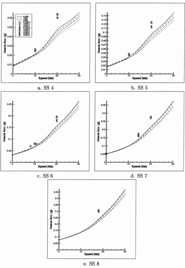
5-6 Mathematical Hull Heave Acceleration . . . 113

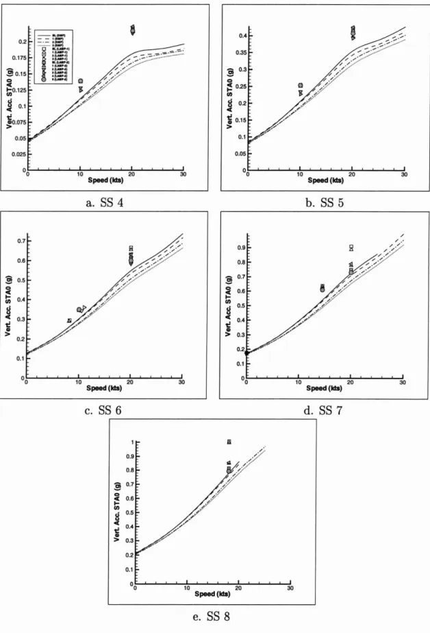
5-7 Mathematical Hull Vertical Acceleration STAO . 114

5-8 Mathematical Hull Vertical Acceleration STA3 . 115

5-10 Mathematical Hull Relative Motion STAO 5-11 Mathematical Hull Relative Motion STA3 5-12 Mathematical Hull Relative Velocity STA3 5-13 Mathematical Hull Relative Motion STA20 . 5-14 Mathematical Hull Deck Wetness STAO . 5-15 Mathematical Hull Slamming STA3 . . .

5-16 Mathematical Hull Propeller Emmersion STA20 5-17 VLCC Heave

5-18 VLCC Pitch .

5-19 VLCC Vertical Shear Force STA5

5-20 VLCC Vertical Bending Moment STA10 5-21 VLCC Vertical Shear Force STA15 5-22 VLCC Heave Acceleration . . . . . 5-23 VLCC Vertical Acceleration STAO . 5-24 VLCC Vertical Acceleration STA3 . 5-25 VLCC Vertical Displacement STA20 5-26 VLCC Relative Motion STAO

5-27 VLCC Relative Motion STA3 5-28 VLCC Relative Velocity STA3 . 5-29 VLCC Relative Motion STA20 . 5-30 VLCC Deck Wetness STAO 5-31 VLCC Slamming STA3 . . .

5-32 VLCC Propeller Emmersion STA20

6-1 V4 Harmonics Comparison (Motions) 6-2 V4 Harmonics Comparison (Loads) . 6-3 V4 Heave RAG's, 20 knots, Head Seas 6-4 V4 Pitch RAG's, 20 knots, Head Seas . 6-5 V4 VSF5 RAG's, 20 knots, Head Seas. 6-6 V4 VBM10 RAG's, 20 knots, Head Seas

117 118 119 120 121 122 123 126 129 132 135 138 141 142 143 144 145 146 147 148 149 150 151 168 169 170 171 172 173

6-7 V4 VSF15 RAG's, 20 knots, Head Seas 174 6-8 VLCC Heave RAG's 178 6-9 VLCC Pitch RAG's. 179 6-10 VLCC VSF4 RAG's 180 6-11 VLCC VSF16 RAG's. 181 6-12 VLCC VBM10 RAG's 182

6-13 VLCC Mean RAG's, (R_{o -} R_{calm )/(2} 183

6-14 VLCC Heave RAG's by Wave Slope. 185

6-15 VLCC Pitch RAG's by Wave Slope 186

6-16 VLCC VSF4 RAG's by Wave Slope 187

6-17 VLCC VSF16 RAG's by Wave Slope 188

6-18 VLCC VBM10 RAG's by Wave Slope . 189

6-19 Harmonics Method Time Domain Comparison: Pitch (SS5, 20kts) 197 6-20 Harmonics Method Time Domain Comparison: VBM10 (SS5, 20kts). 198 6-21 Harmonics Method Time Domain Comparison: Pitch (SS7, 20kts) .. 199 6-22 Harmonics Method Time Domain Comparison: VBM10 (SS7, 20kts). 200 6-23 Normal Distribution Analysis, V4, Pitch & VBM10, SS5 20kts 203 6-24 Normal Distribution Analysis, V4, Pitch & VBM10, SS7 20kts 204

List of Tables

2.1 Selected Seakeeping Criteria for Naval and Commercial Hulls. 25

2.2 U.S. Navy Sea State Standards 27

2.3 LAMP and SMP Formulation Comparison 36

2.4 Measured Responses in LAMP and SMP 44

3.1 Mathematical Hull Main Particulars. . . 59

3.2 Mathematical Baseline Static Load Limits 61

3.3 VLCC Hull Main Parameters 65

3.4 VLCC Static Load Limits . . 66

4.1 McCreight Ranks of Mathematical Hulls . . . 72

4.2 Out-of-Range Geometry Factors for McCreight Index 73

4.3 Mathematical Hull Naval Criteria Limiting Speeds (SMP) 77

4.4 SPI (Naval Criteria) of Mathematical Hulls. . . 78

5.1 Mathematical Hulls LAMP Irregular Seas Run Summary 87

5.2 VLCC LAMP Irregular Seas Run Summary . . . 87

5.3 V4 Prediction Comparison, Irregular Seas (SS6, 10 kts) 94

6.1 Mathematical Hull LAMP Regular Waves Run Summary 161

6.2 VLCC LAMP Regular Waves Run Summary . 162

6.3 V4 Method Comparison - Heave. 192

6.4 V4 Method Comparison - Pitch . 193

6.5 V4 Method Comparison - VSF5 . 193

6.7 V4 Method Comparison - VSF15 . . . .

7.1 Relative Clock Time Comparison - V4 and VLCC Analyses

194

Nomenclature

ABS AWA B BL BML

C

B CDF CFD

CG

C

J CVPA

C

VPF D DDG DOD DWL FFG FFT FP Fr 9

American Bureau of Shipping Waterplane Area, Aft of Midships Molded Beam

Mathematical Hull Baseline Longitudinal Metacentric Radius Block Coefficient

Cumulative Distribution Function Computational Fluid Dynamics Center of Gravity

Waterplane Inertia Coefficient,

=

BML

\7/

BL3

Vertical Prismatic Coefficient, Aft of Midships Vertical Prismatic Coefficient, Forward of Midships Molded Depth

Guided Missile Destroyer Department of Defense Design Waterline Guided Missile Frigate Fast Fourier Transform Forward Perpendicular Froude Number, V/VgLBP Gravitational Acceleration Significant Wave Height Wave Height

'l

KG

kxx

k

yy L LAMP

LBP

LCB

LCF

LCG

LMPRES

LOA

Lw LWL MSF MSI NTU 01 POSSE R1

RAO

RMS

ROE

s SA SAIC SHCP SIG SMP

ith harmonic (1,2,3, ... ), 0

=

mean response,

calm

=

calm water steady state value Height of Center of Gravity above the Keel Mass Transverse Radius of Gyration

Mass Longitudinal Radius of Gyration Length (LWL unless otherwise specified) Large Amplitude Motions Program Length Between Perpendiculars Longitudinal Center of Buoyancy Longitudinal Center of Flotation Longitudinal Center of Gravity LAMP Pressure Post-Processor Length Overall

Wave Length

Length of the Waterline Mixed Source Formulation Motion Sickness Indicator National Taiwan University Operating Index

Program of Ship Salvage Engineering McCreight Rank

Response Amplitude Operator Root Mean Square

Response Operating Envelope Sample Standard Deviation Single Amplitude

Science Applications International Corporation Ship Hull Characteristics Program

Significant One-Third Response Ship Motions Program

SOE SPI SPI-1 SPI-2 SS STA T

v

Vx VBMx VBMxi VLCC VSFx VSFXi

z·

z K-3 w

Seakeeping Operating Envelope Seakeeping Performance Index Mission Effectiveness Index Transit Time Index

Sea State Ship Station Molded Draft Modal Wave Period Ship Velocity

Mathematical Hull Variant x

Total Vertical Bending Moment at Station x

Vertical Bending Moment at Station x, ith harmonic Very Large Crude Carrier

Total Vertical Shear Force at Station x

Vertical Shear Force at Station x, ith harmonic Sample Mean

Heave Response, ith harmonic Displacement

Wave Amplitude

Total Disturbance Potential Incident Wave Potential Total Velocity Potential Skew

Kurtosis

Population Mean

Population Standard Deviation

(a

2 _{= Variance)}

Pitch Response, ith harmonic Absolute Wave Frequency

Wave to Ship Encounter Frequency Volumetric Displacement

Chapter

1

Introduction

Hydrodynamics is a critical part of the ship system design process, directly or indi-rectly impacting nearly every other engineering aspect. Hydrodynamic design areas include ship resistance, propulsor design, seakeeping, maneuvering, and the dynamic impacts on hydrostatic stability. However, properly incorporating hydrodynamics in ship design is one of the most difficult tasks confronting the engineer. The fl uid-ship interaction is an extremely complicated one and difficult to accurately predict. As a result, designers often rely on empirically based parametric data or simplified calculation methods during the early stages of design. As the design progresses, ex-perimental model tests are often used to confirm the hydrodynamic characteristics of the hull. Because model testing involves the production of physical scale models and the use of large laboratory facilities, experiments can be quite costly. The high expense can force delay of model tests until late in the design process, and accu-rate hydrodynamic predictions transition from design to merely analysis tools. Any changes required in the ship hull form at this stage are likely to be far more expensive than if the deficiencies were predicted earlier.

The widespread availability of powerful high speed computers offers the oppor-tunity to include accurate hydrodynamic analyses much earlier in the ship design process. Recently researchers have made significant efforts towards accurately pre-dicting fluid flow around ships and appendages. Advances in numerically solving both inviscid potential flow fields and viscous laminar and turbulent flows using high

performance computers are now beginning to fill the design gap between early design methods and experimental studies. Computer methods are available for predicting ship resistance, propulsor performance, details of viscous flows around ships and sub-marines, and seakeeping.

Seakeeping, particularly, is a critical area of ship design. VADM R.E. Adamson, Jr., U.S. Navy, operationally defined seakeeping in 1975, while Commander, Naval Surface Forces Atlantic [1]: "Seakeeping, as it pertains to the U.S. Navy, is the ability of our ships to go to sea, and successfully and safely execute their mission despite adverse environmental factors." This definition of seakeeping is not merely naval -commercial ships too must execute their economic mission in harsh environments, although particularly severe seas may be avoided, which may not be possible in mil-itary scenarios. Technically, seakeeping involves the prediction of ship motions and structural loads which are induced by the hull's encounter with water waves. No matter the ship's mission, seakeeping will have an important impact on the ability to perform that mission. Seakeeping is arguably the most critical of all hydrodynamic sub-disciplines due to its impact on ship survivability, particularly in heavy to se-vere seas. This research concentrates on the seakeeping sub-discipline because of the severe risks to ships in dangerous seas.

Very early stage ship seakeeping design has traditionally relied on empirically-based parametric estimates of ship motion and load response amplitudes. For naval destroyer type hulls, designers often use ranking systems developed separately by Bales [2] and McCreight [3]. Each of these researchers statistically regressed key seakeeping response amplitudes as functions of ship underwater geometry. The same parameters of a new ship hull can be used to relatively compare predicted seakeeping performance as a single index value. These method are discussed further in Chapter 2. Other researchers, notably Loukakis and Chryssostomidis, have developed series for early prediction of ship seakeeping [4]. These series can be used in a similar fashion as the well-known resistance prediction method, the Taylor Standard Series. The Loukakis and Chryssostomidis series predicts motions and loads of ships with cruiser sterns as a function of beam to draft ratio (BIT), length to beam ratio (LIB), and

block coefficient (CB) .

For the next stage of seakeeping design, the use of linear strip theory predictions for motion and loads in the frequency domain is now widely accepted among naval architects as an early stage design tool. Salvesen, Tuck, and Faltinsen developed strip theory into a viable design calculation method for ships [5]. Their effort led to the current frequency domain calculation programs. Two of the most prominent of these are the U.S. Navy's Ship Motions Program and the MIT RA05D code. Frequency domain programs can quickly calculate ship responses at a large number of speeds, headings, and wave conditions, and are thus ideal for early design, where a large number of hull alternatives may require analysis.

There are limits to the usefulness of parametric and frequency domain prediction methods in seakeeping design. Most parametric methods, including those of Bales and McCreight, are based on characteristics of the mean underwater hull form. Geometry factors above the calm waterline, such as flare or tumblehome, do not influence a ship's performance rank. Only a limited number of geometric parameters are used to predict performance. Some methods, such as the cruiser stern series use only length, beam, draft, and volumetric displacement as inputs. Additionally, if any hull or envi-ronmental characteristics fall outside the range of tested conditions, the extrapolated results may be questionable. Linear frequency domain codes also function on the assumption that ship responses to encountered waves may be linearly superposed to yield the total response. Again, only the mean underwater hull form is considered. Significant variations in above water geometry will affect the prediction accuracy. Additionally, the frequency domain programs linearize by assuming small wave and motion amplitudes. Sea states or ship characteristics which result in large amplitude motions or loads violate the conditions of this linearization. The linear predictions will break down in cases where seakeeping performance is most critical- where large amplitude responses seriously degrade ship performance or even threaten survival.

To overcome these problems, towing tank tests are traditionally performed later in design to predict vertical motions (heave and pitch) and loads in head seas, and possibly horizontal motions (especially roll) in oblique seas. As mentioned above,

these experimental tests are expensive. Again, changes in hull form at the stage of tank tests are more costly and have a larger effect on the rest of the ship design.

To overcome these difficulties, the prediction of wave-induced motions and loads in the time domain has been the primary goal of many of the recent computer advances in ship hydrodynamics. Efforts have ranged from nonlinear time domain implementation of strip theory, such as discussed by Burton, et al. [6], to the solution of the nonlinear three-dimensional problem. One example of the latter is the Large Amplitude Motions Program (LAMP) developed by the Ship Technology Division of Science Applications International Corporation (SAIC). The theory and some results of the LAMP code have been presented in several papers [7, 8, 9, 10]. A brief review of the theory and formulations of LAMP is given in 2.

With the availability of such time domain prediction methods, the obvious ques-tion to any ship designer should be: "How do I use them?" This research explores that question. A possible design progression which incorporates parametric, frequency domain, and time domain methods is proposed. Two types of hulls are considered. The first type consists of a series of six mathematically defined hull forms, based on the well-known Wigley seakeeping hull. While primary dimensions of the ship

(L,

B, T, and CB) are fixed, two parameters important to seakeeping - flare angle and

waterline entrance angle - are varied both above and below the mean waterline. Two hulls are different from the baseline Wigley hull only above the waterline - one with flare, and the other with tumblehome. These hulls are particularly interesting in that parametric and linear methods predict exactly the same performance as the baseline. A commercial Very Large Crude Carrier (VLCC) hull is also examined.

Each hull is analyzed in the frequency domain with SMP, and in the time domain with the different implementations of LAMP. All hulls were tested in irregular seas in the frequency and time domains. Regular wave runs to determine Response Am-plitude Operators (RAO's) were also conducted in the time domain. The results of the different calculation methods are compared. Finally, recommendations are made for the use of time domain codes in seakeeping design, discussing both the results of this research and several other applications not examined explicitly here.

Chapter

2

Design Method

Incorporation of seakeeping in the ship design process requires the selection of reason-able performance criteria, which typically consist of a series of motion and structural load limits. The ship's ability to meet these performance criteria is then analyzed in sea states corresponding to the expected operating environment of the vessel. Chapter 2 discusses the selected performance criteria and operating environments for both the mathematical and commercial hulls and the prediction tools selected for comparison. Finally, a proposed method for incorporating time domain predictions in the design procedure is presented.

2.1

Performance Criteria

2.1.1

Motion Limits

The first step in measuring the seakeeping performance of a ship is the establishment of motion (and load) limits, beyond which occurs degradation of one or more aspects of the total ship system. These criteria apply in any sea state, ship speed, or heading with respect to the waves. Motion criteria can generally be grouped into two cate-gories: primary and derived. Primary criteria include the basic ship motions - surge, sway, heave, roll, pitch, and yaw - and their velocities and accelerations. Motions at a point other than the ship center of gravity (CG) are also considered primary criteria

as they are fully defined by the six basic motions. Derived criteria can actually be more critical in their degradation of the ship's mission. These criteria include relative motions at a point, defined as the difference between the amplitude of the vertical point motions (displacement, velocity, or acceleration) and the wave motion (again, displacement, velocity, or acceleration) at that point. Several other derived responses are themselves functions of relative motion, including deck submergence (wetness), emergence (such as at the propeller), and slamming. Slamming occurs when the ship emerges out the water at a point, and reenters the water above a threshold relative velocity. A motion sickness indicator (MSI) is also available to estimate the likely percentage of sea sickness among the crew. Excellent descriptions of the motion limits are available in Lewis, 1989 [11] and Bhattacharyya, 1978 [12].

Appropriate naval motion limits for design have been well defined by Comstock, et al., 1980 [13], and recommended as a U.S. Navy (USN) design standard [14]. Motion criteria are established for each warfare mission of naval ships, e.g. anti-air warfare, anti-submarine warfare, and aviation operations. For purposes of this study, the recommended criteria for transit operations are used to define ship requirements. These criteria are summarized in Table 2.1 on the facing pagea.

For transit missions, the deck wetness and slamming limits define conditions where damage to the ship hull or deck equipment could occur. The roll, pitch, and accel-eration criteria define conditions where the ability of ship's personnel to function effectively would be degraded. The acceleration conditions typically are applied at the vessel's bridge - station! 3 is used as a conservative typical position. USN stan-dards for ship-equipment interface also define the level of dynamic forces which all shipboard equipment must be designed to encounter [17]. For the mathematical hull, the personnel-related acceleration limits are exceeded before the equipment interface standards, therefore only the personnel standards are considered.

Commercial ship criteria are less well-defined than naval criteria. However, Aertssen, et al. (1968, 1972) studied the the seakeeping performance of several commercial ships and proposed appropriate design criteria [15, 16]. These criteria are prescribed for

Criteria Naval Monohull (Transit)

Roll

(0)

8.0

Pitch

(0)

3.0

Vert. Accel. (g) STA3 0.4

Lat. Accel. (g) STA3 0.2

Slam Freq. STA3 20/hr.

Dk. Wetness STAO 30/hr.

Note: Significant 1/3 Single Amplitudes

a. Naval Transit Criteria [14, 13]

Criteria Bulk Carrier

(Transit)

Vert. Accel. (g) STA3 0.5

Slam Accel. (g) STA3 0.2

Slam Freq. STA3 3/100

Dk. Wetness STAO 5/100

Prop. Emergence STA20 25/100 Note: RMS Single Amplitudes

b. Commercial Transit Criteria [15, 16, 11, p.143]

Table 2.1: Selected Seakeeping Criteria for Naval and Commercial Hulls

typical vessels in Principles of Naval Architecture [11, p. 143]. The Aertssen criteria for bulk carriers are applied to the VLCC hull in this research, and are summarized in Table 2.1b. Note that the selected naval criteria are defined as the average of the highest one-third response amplitudes ("Significant Single Amplitude (SIG SA)"). The commercial criteria are the root mean square response amplitudes (RMS SA).

2.1.2

Structural Load Limits

Motion criteria are relatively easy to define since they typically correspond to an observable response, e.g. motion of the ship, or wetness of the foredeck. Structural load limits, however, are more difficult to quantify since the stresses of the ship are not immediately discernible until failure occurs, unless strain measuring devices

are installed for real time feedback to the ship's operators. In early ship design, initial scantling sizes are traditionally estimated based on projected vertical bending moments and shear stresses. These moments and stresses are calculated based on the ship's longitudinal buoyancy and weight distribution. Besides the still water condition, both naval and commercial criteria typically require the calculation of maximum design stresses which are expected to occur in both a severe hogging and severe sagging condition.

For USN ships, the hull is balanced on a trochoidal wave, with the length of the wave equal to the ship's length, Lw

=

LBP, and the height of the wave defined as

Hw = 1.1JLBP[feet]. For the design hogging condition, the wave is centered on the

ship with the crest at amidships. For the sagging condition, crests are positioned at the perpendiculars. After weight and buoyancy are balanced in each condition, the shear stresses and bending moments are calculated along the length of the ship. The resulting stresses are the design maximums for initial structural definition [18].

For commercial ships, various criteria typically apply, dependent upon the ship's classification society, flag nation standards, etc. A typical criteria is that used by the American Bureau of Shipping (ABS) [19]. These det6fministic rules are semi-empirical functions of ship length, beam, and block coefficient which estimate addi-tional shear stress and bending moment in sagging and hogging conditions.

Both the USN and ABS criteria are static and so often criticized for represent-ing deterministic solutions to what is realistically a probabilistic problem. ABS is implementing probabilistic criteria through its Safehull software. Though still deter-ministic, the Navy static wave balance is supplemented by the additional inclusion of stresses due to wave slap, water on deck, and other secondary loads. Dynamic stresses due to ship motion are included with guidelines such as the DOD-STD-1399, discussed above.

There are several other categories of structural loads that must be considered dur-ing design. Besides the vertical shear stresses and benddur-ing moments, both horizontal and torsional loads should be considered as primary hull girder loads. Severe local loads can also occur due to wave hydrostatic and hydrodynamic pressure. Slamming

Sea Significant Wave Percentage Modal Wave Period (sec)

State Height (m) Probability Most

Number Range Mean of Sea State Range Probable

o-

1

o-

0.1 0.05 0 - -2 0.1 - 0.5 0.3 5.7 3 - 15 7 3 0.5 - 1.25 0.88 19.7 5 - 15.5 8 4 1.25 - 2.5 1.88 28.3 6 - 16 9 5 2.5 - 4 3.25 19.5 7 - 16.5 10 6 4-6 5 17.5 9 - 17 12 7 6-9 7.5 7.6 10 - 18 14 8 9 - 14 11.5 1.7 13 - 19 17 >8 >14 >14 0.1 18 - 24 20

Table 2.2: U.S. Navy Sea State Standards [14]

can create severe local loads and ship whipping responses. Finally, the fluctuations of stresses due to these load factors are an important consideration in fatigue prevention.

Many of these additional loads are not currently predicted well. Such calculations are one potential benefit of nonlinear time domain methods and are discussed briefly in Section 7. However, as a reference load limit during this research, the USN static wave balance is applied to the mathematical hulls, and the ABS limit to the VLCC hull. The structural limit calculations are further discussed in Sections 3.1.4 and 3.2.1.

2.1.3

Operating Environment

Seakeeping performance is dependent on the ship hull, the ship's operating profile (speeds and headings, discussed in Section 2.1.4), and the sea environment. The sea conditions are typically defined by sea state, representing expected wave heights, wave modal periods, and wind speeds. Table 2.2 represents standard sea conditions in the winter North Atlantic, and is recommended for design by the U.S. Navy [14]. Expected wind conditions are not included, since none of the selected motion or load criteria are explicitly wind dependent. Performance criteria for aviation operations are strongly wind dependent. Comstock, et aI., performed a thorough study of the

seakeeping characteristics of naval aviation-capable ships using wind criteria in 1982

[20].

For this research, sea states 4 (moderate) through 8 (severe) are considered. A Bretschneider two-parameter spectrum is used to define each sea state based on the most probably significant wave heights and modal periods, so that:

S(w)

=

486.0·HITo-4w-5e-1948.18.To-4w-4

3

Only long-crested unidirectional seas are considered in the seakeeping assessments.

2.1.4

Seakeeping Measures of Performance

Once the ship's motion and load limits are established, and the operating environment defined, the ship's seakeeping performance is evaluated at each desired condition. Two well-established methods for quantifying overall seakeeping performance are the Mission Effectiveness Index (SPI-l) and the Transit Time Index (SPI-2) [11].

Mission Effectiveness Index (SPI-l)

The SPI-l is the percentage of time that a ship in a given condition can perform its military or commercial mission, given a projected operating environment. Per-formance of a mission assumes that no motion or load limits are exceeded. SPI-l is calculated in the following manner:

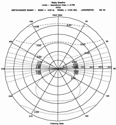
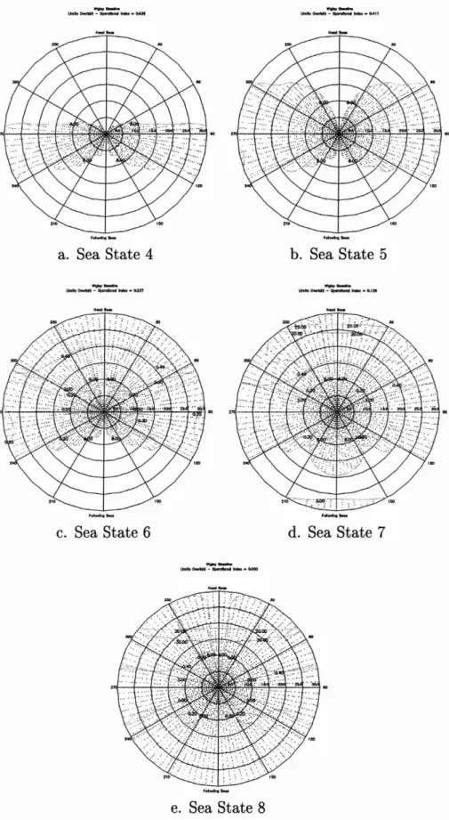
1. Calculate the ship's motions and loads in each sea state of interest, over all possible speeds and headings with respect to the waves. For each motion, the data are often presented in a speed polar format, such as in Figure 2-1 on the next page. Here, the significant one-third pitch amplitude in sea state 6 for the mathematical baseline of this study (Wigley Seakeeping Hull) is contour plotted, as calculated by the frequency domain program SMP. The radial axis is ship's speed in knots. The angular axis is heading with respect to the waves. For each motion, the appropriate limits are overlaid. In Figure 2-1, response contours above the pitch limit of 3° are dashed. Ifall speeds and headings are

W1gleyBa...

Umlt. - Operational Index - 0-7511 PITCH

BRETSCHNEIDER S£AWAY - SlGWH - 5-00 IL 'IlI0lW. - 13.00 SEC. LONGCRESTED SIC SA

FollowinllS

-Figure 2-1: 8peed Polar Plot, Mathematical Baseline, Pitch (886)

weighted equally, the Response Operating Envelope (ROE) for pitch in this case is 0.759. The ROE indicates that the Wigley Baseline does not exceed pitch limits in 886 at 75.9% of all possible speeds and headings.

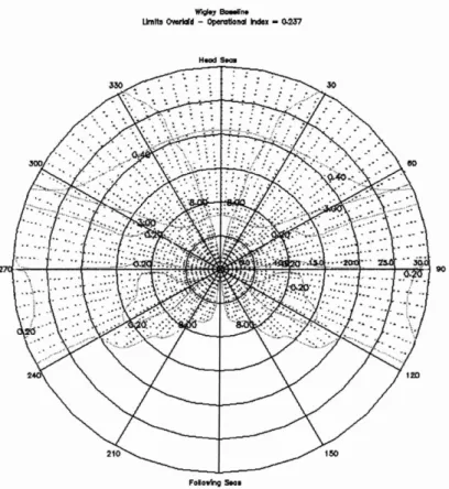
2. For each mission, all of the applicable ROE's are overlaid for each sea state. Again for 8S6, the naval transit limits defined in Section 2.1.1 are overlaid against ship response and plotted in Figure 2-2 on the following page. Dotted areas indicate speeds and headings where one or more of the transit motion limits are exceeded. The Seakeeping Operating Envelope for each mission in each sea state is the intersection of all the applicable ROE's. The 886 Transit 80E is only 23.7%, limited primarily by roll in addition to pitch. One of the primary strengths of the 8PI-1 method is that each speed-heading combination can be weighted by its probability of occurrence in the ship's expected operating profile. The Operating Index (01) for the mission is then the 80E weighted

Heads.a.

Folow1nv SM.

Figure 2-2: 8peed Polar Plot, Mathematical Baseline, Naval Transit Mission (886)

by the speed-heading probabilities. In this example, however, all speeds and headings are weighted equally, and the 01 equals the 80E. Mathematically, for the transit mission,

Oli

=

L L SOE· Wj

Speed Heading

where Wj is the probability of each speed-heading.

3. Next, the 01 for each mission area in each sea state is weighted by the probability of that sea state, yielding a total mission 01. The mission OI's are then weighted by the mission importance to yield 8PI-l, or:

i j

SPl= L miLOli'Pj

Missions SS

where mi is the mission weighting, and Pj is the sea state probability, defined in Table 2.2 on page 27.

For military ships, SPI-l is particularly well suited for seakeeping comparison because both the speed-heading operating profile and the mission importance can be included. Frequency domain programs, like SMP, are particularly well suited for the calculation of SPI-l, due to their calculation speed. All speed-heading combinations can be quickly calculated.

Transit Time Index (SPI-2)

The transit time index, or SPI-2, is defined as the amount of time a given distance would take to travel in calm water, divided by the amount of time the same trip would take in the actual sea environment. Alternatively, the expected speed fraction is used, which is the ratio of actual maximum speed to calm water maximum speed for a given transit route [11]. SPI-2 is often used for commercial ship analysis, where port-to-port transit time is the primary concern. When analyzing transit missions for naval ships, SPI-2 is also applicable.

Unlike SPI-l, SPI-2 considers both involuntary and voluntary speed losses. In-voluntary speed losses are caused by added resistance in waves and loss of propulsor efficiency due to the sea environment and wave-induced motions. Voluntary speed losses are considered under the assumption that the ship's operators would change either speed or heading if any motion limits were exceeded at their current speed and heading. For military ships particularly, this assumption would not always be true -depending on the tactical situation, the ship may need to perform a mission at any speed or heading, even if performance is degraded by motions or loads. For moderate to high speed ships, the involuntary speed losses are typically small compared to the voluntary speed losses, and are often neglected.

To calculate SPI-2, SOE diagrams for the transit mission in each sea state are prepared as above. For each heading in each sea state, the maximum speed at which transit is possible without voluntary speed reduction is recorded. Finally, the max-imum speed is weighted by the ship heading probability with respect to the waves for each sea state. The weighted average maximum speed for each sea state is then weighted by the probability of occurrence for each sea state, and summed to yield the

average expected speed. This speed is divided by the ship's maximum speed, yielding the expected speed fraction. This method applies if the minimum distance route is taken, regardless of possible routing around bad weather. If that assumption is not true, the transit time fraction should be used.

For purposes of this research, only the transit missions of the mathematical (naval criteria) hulls and the VLCC are considered. Thus, SPI-2 is an appropriate measure of seakeeping performance. Additionally, only head seas are considered (discussed in Section 2.3.2), so that the expected speed fraction is calculated for head seas. Hereafter, SPI refers to SPI-2, unless otherwise specified.

2.2

Prediction Tools

With the motion and load criteria defined, and the head-seas only SPI selected as the performance index for frequency and time domain calculations, the different predic-tion methods in the study are now considered.

2.2.1

Parametric

Empirical or semi-empirical parametric prediction methods are often the first sea-keeping evaluation tool used in the ship design process. By definition, parametric tools use the known characteristics of similar ships to interpolate for the unknown seakeeping performance of the current ship.

Two of the most common parametric methods in naval monohull seakeeping de-sign are those proposed by Bales in 1980 [2] and by McCreight in 1984 [3]. Bales considered the head seas seakeeping performance of twenty destroyer-type hulls over a range of operating speeds in various sea states. He developed a performance index (the Bales Index) which is a function of eight responses: heave, heave acceleration, pitch, relative motion at the bow, absolute vertical acceleration at the bow, absolute vertical displacement at the stern, relative motion at the stern, and a slamming co-efficient measured at Station 3. The performance of each ship was then regressed as a function of several key hull geometry parameters, including: waterplane area

coef-ficients forward and aft of amidships (CWF and CWA ), draft-to-Iength ratio (T/ L),

vertical prismatic coefficient forward and aft of amidships (CVPF and CVPA ) , and

cut-up ratio (c/

L).

Cut-up (c) is the distance from the ship's forward perpendicu-lar to the point where the keel begins to rise above the baseline towards the stern. Displacement was not explicitly considered, as all tested ships had full scale displace-ments of about 4300 metric tons. A ship's final index score is calculated based on its geometric properties, and can then be adjusted for its displacement.

McCreight expanded on this method in 1984. While considering the same list of important seakeeping responses, he tested twenty-five hulls in addition to the original Bales series, extending the applicable range of hull parameters. Regression of sea-keeping performance was attempted for several additional hull parameters, including volumetric displacement (V). Additionally, cut-up ratio was eliminated as a param-eter. The resulting regression equation for the McCreight Index is:

where:

R

I is the McCreight Rank, BML is longitudinal metacentric radius, AwA

is waterplane area aft of amidships, LCB is longitudinal center of buoyancy, LCF is longitudinal center of flotation, and CJ is a waterplane inertial coefficient, equal

to BMLV /BL3. The regression coefficients, ai, are available in [3]. The McCreight

Rank calculation is performed for each of the mathematically defined hull forms in Chapter 4.

Parametric methods such as the Bales or McCreight ranks, or series such as the Loukakis and Chryssostomidis seakeeping study [4], are very useful for extremely early design in selecting primary hull dimensions which generally will improve seakeeping. However, like linear methods, the above water hull is not considered, and any other variations from the hulls of the empirical database reduce their usefulness in design.

2.2.2

Frequency Domain: SMP

After parametric methods, the next step in seakeeping design is typically the use of linear frequency domain methods based on two-dimensional (2-D) strip theory. Their usefulness has already been demonstrated through the rapid preparation of speed polar plots such as those in Section 2.1.4. The frequency domain program used to predict motions and loads for the mathematical hulls and VLCC in this study is the U.S. Navy standard, Ship Motions Program, 1995 version2 _(SMP95).

Linearized strip theory programs, such as SMP and the MIT RA05D program, were developed based on the calculation methods of Salvesen, Tuck, and Faltinsen [5]. Strip theory methods, though extremely useful for early design, suffer from the failure of the linear assumption for certain hulls and sea conditions. 2-D strip theory requires that the ship length be much greater than both the beam and the draft, so that end effects are not important in the potential flow solution. The SMP user's manual warns that prediction accuracy is degraded when L/B

<

5 [21]. Addition-ally, linearization requires that the properties of the hull sections and waterplanes throughout the range of motion be well represented by the calm water values. Hull geometry above the calm waterline, including flare or tumblehome, does not affect the solution. The linearization assumption thus requires that ship motions be limited to small amplitudes. SMP again specifically warns that prediction accuracy degrades for wave heights greater than ship's draft,.

Finally, the linear frequency domain method assumes that the ship's response to a system of waves (such as irregular seas) is simply the sum of the responses to each individual wave, through superposition. Only the first order response is considered. For vertical motions or loads like heave and pitch, this assumption is often valid as long as motion amplitudes remain small. For lateral motions or loads, such as roll, however, the linear assumption is typically not valid. SMP applies a weakly nonlinear correction to model hull and appendage lift viscous damping based on the

2SMP95 was used for regular and irregular wave predictions for the mathematical hulls, and irregular seas prediction for the VLCC. VLCC regular waves predictions were actually performed first chronologically, using SMP91. Load RAG's were not calculated for the VLCC due to a known error in the SMP91 loads algorithm, which was corrected in SMP95.

significant roll amplitude. During irregular seas calculations, an iterative procedure for roll response is implemented.

As long as the assumptions of the the linearized 2-D solution are valid, programs like SMP are extremely rapid, useful tools. The recommended design procedure outlined in Section 2.3 uses linear frequency domain programs to narrow down the conditions which warrant nonlinear time domain analysis. Using regular wave anal-ysis, the linear prediction of zero higher order response is also examined in Chapter 6.

2.2.3

Time Domain: LAMP

The Large Amplitude Motions Program (LAMP), developed by the Ship Technol-ogy Division of Science Applications International Corporation (SAlC) , was used to perform all time domain calculations for this study. LAMP is representative of cur-rent computational fluid dynamics (CFD) codes for the prediction of nonlinear ship motions and loads in the time domain. A brief review of the LAMP methodology provided here is similar to the description found in Shin, et al. (1997) [9]. More detailed descriptions of the LAMP theory are available in the LAMP User's Manual, and in Lin and Vue (1990) [22, 7].

LAMP computes a time domain solution for a general three-dimensional body floating on a free surface. Six degree-of-freedom motions are permitted. In the most advanced formulation, the complete hydrodynamic, hydrostatic, and Froude-Krylov potential solution is calculated at each time step on the ship's instantaneous under-water hull form. Note that this is a major difference from linear methods, where only the mean underwater body is considered. The wave pressure forces are combined with any external forces to solve the equations of motion at each time step. The hull pressure forces may also be used to calculate hull bending and torsional moments and shear forces. Due to the complexity of applying the fully nonlinear body boundary condition, several different formulations have been developed. These formulations, along with SMP, are compared in Table 2.3 on the following page.

SMP 2-D Linear Hydrodynamics (Strip Theory)

Linear Hydrostatic Restoring and Froude-Krylov Wave Forces Frequency Domain

LAMP-l Free Surface Boundary Condition on Mean Water Surface 3-D Linear Hydrodynamics

Linear Hydrostatic Restoring and Froude-Krylov Wave Forces LAMP-2 Free Surface Boundary Condition on Mean Water Surface

3-D Linear Hydrodynamics

Nonlinear Hydrostatic Restoring and Froude-Krylov Wave Forces LAMP-4 Free Surface Boundary Condition on Incident Water Surface

3-D Nonlinear Hydrodynamics

Nonlinear Hydrostatic Restoring and Froude-Krylov Wave Forces Table 2.3: LAMP and SMP Formulation Comparison

The computations are much less intensive, but the results still suffer from the disad-vantages inherent with the mean body boundary condition. However, the limitations of 2-D methods do not apply. Additionally, simply switching to the time domain eliminates the requirement for the linear superposition assumption required by fre-quency domain methods. For large-amplitude responses, this difference should be quite significant. LAMP-4 is the fully nonlinear implementation, solving the under-water potential solution on the instantaneous hull surface. However, LAMP-4 is far more computationally intensive than LAMP-I. LAMP-2 is an approximate nonlinear method which retains many of the advantages of both LAMP-l and LAMP-4. In this formulation, the hydrodynamic potential is still solved on the mean underwater body, but the hydrostatic and Froude-Krylov wave forces are applied to the instantaneous underwater body. In head seas and vertical motions, where these forces typically dominate, LAMP-2 may be very useful.

The mathematical implementation of the LAMP method is discussed briefly below. The fluid motions are described by a velocity potential

~T(X,

t)

=

~I(X,

t)

+

~(x,

t)

to the presence of the ship.

x

is a position vector and t is time. The velocity potential must satisfy Laplace's equation,

The disturbance potential solution must satisfy the free surface and body bound-ary conditions, along with a radiation condition. The free surface boundbound-ary condition is linearized in all three formulations, such that

on

where g is gravitational acceleration. The body boundary condition is next applied on the instantaneous underwater body for LAMP-4 and the mean underwater body for LAMP-l and LAMP-2,

on

wheren is a unit normal vector to the body out of the fluid andVn is the instantaneous

body velocity in the normal direction. Obviously, 8b

(t)

is constant for LAMP-l and

2. Next, the radiation conditions require that the disturbance velocity potential goes to zero at infinity, 800 ,

8<I>

<P=--+O

at

on 800 ,t

>

0

Finally, the initial conditions require a zero disturbance potential on the free surface at t = 0,

a

<I> <I>=-=O

at

on

Two methods have been included in LAMP to solve for the potential function,

<I>(t)

at each time step. The first uses a transient free-surface Green function (Go

+

Gf),

with homogeneous singularities placed on the hull surface only. This formulation, along with the boundary conditions is graphically summarized in Figure 2-3a, from

a. Transient Green Function Formulation

s

00

b. Mixed Source Formulation Figure 2-3: LAMP Formulations [22]

the LAMP User's Manual. A mixed source formulation (MSF), recently developed, is summarized in Figure 2-3b. Inthis method, the fluid is split into two domains (1 and 11). The MSF distributes simple Rankine sources (G) on the hull, local free surface, and a matching surface, Sm, between the two fluid domains. A transient Green function is applied on the matching surface. Both SAIC testing and the author's experience with both the VLCC and mathematical hulls in large-amplitude motion cases indicate that the MSF is more robust, particularly with non-waIl-sided hull geometries [23]. Consequently, the mixed source formulation was used in all LAMP runs.

LAMP provides the user with several other options affecting the time domain solution method. For the MSF, two options for the inner boundary of the free surface panelization are available. For both methods, the hull matching surface is used as the outer edge of the free surface panelization. In the first method, the actual hull waterline is used as the inner boundary of the free surface, yielding a "body-fitted" free surface grid. In the second, a shifted and scaled copy of the matching surface is used as the inner boundary, resulting in minimized gaps between the hull and free surface grid. For all LAMP runs, the body-fitted method was used. However, some LAMP-4 runs were attempted unsuccessfully with the gapped method. This is discussed in Section 5.2.3.

Two methods are also available for cutting the panelization of the hull at the mean waterline. In the default method, component cutting, the intersection of the mean or incident free surface is calculated at each station. The underwater station is then resplined with the same number of points at each time step. The alternate method, master geometry cutting, does not respline stations under the free surface. Submerged panels are maintained, and panels at the waterline are trimmed off. The component cutting method was used for all LAMP-l and LAMP-2 runs, which use the mean underwater body regardless. Because the hulls were tested in cases likely to have large-amplitude motions, the master geometry cutting method was used in most LAMP-4 cases. Some VLCC cases, with less severe motions than the smaller mathematical hulls, used component cutting in LAMP-4. The comparison is briefly discussed in Section 6.3.

Calculation of the pressure from the potential flow solution can also be linearized by dropping the nonlinear second order term in Bernoulli's equation, ~1\7~12. The pressure linearization speeds up calculation, particularly for LAMP-4, and generally results in negligible differences for head seas cases. The linearized method was used for all cases, after consultation with SAIC.

Finally, for all head seas cases, the hull was fixed in all directions except heave and pitch, which is also a normal experimental setup. Additional details of the LAMP setup for each hull are included in Sections 3.1.5 and 3.2.2.

2.3

Time Domain Methods in Design

Because of the increased computation time required for 3-D time domain runs, apply-ing them in the same manner as current frequency domain programs is not feasible. In fact, to test a transversely symmetric hull from zero to thirty knots (five knot increments), in head to following seas (15° increments) would take ninety-one runs per sea state. In this section, two alternative methods of incorporating time domain runs in design are proposed. The first is to use time domain codes (hereafter, LAMP) to verify the frequency domain (hereafter, SMP) predictions for the SPI. The second is to use LAMP as a simulated experimental testing facility.

2.3.1

Seakeeping Performance Index Verification

Once SMP is used to calculate either SPI-1 or SPI-2 for a hull, LAMP can be used to verify the critical points in each ROE or SOE. These critical points are the speeds and headings where either motions or loads first exceed the threshold. For example, referring again to Figure 2-1 on page 29, the pitch ROE of the mathematical baseline in SS6, LAMP could be used only at the speeds and headings where the pitch limit of 3° is exceeded. Assuming 15° heading increments, the hull would be tested at 000, 015, 030, 045, and 060, for a total of only five runs. The speed at each heading would initially be the SMP predicted crossover speed. Using an appropriate iteration scheme, only a few additional runs at each heading should be required to define the ROE.

To reduce the number of required runs even further, LAMP may be used to verify the SOE, where all motion and load limits for a single mission are overlaid, as in Figure 2-2 on page 30. To verify the SS6 Transit Mission SOE, LAMP tests would be conducted at: (1) 000 to verify pitch limit crossover, (2) 180 to verify 30 knots is feasible, and (3) 120, 135, 150, and 165 to verify roll limit (8°) crossover. A total of six initial runs would be necessary, with follow-on runs for iteration to the actual limit crossover speeds.

Testing Application of SPI Verification Method For this study, a modified SPI (transit speed limit) for head seas only is calculated for the mathematical hulls and the VLCC. This reduces the number of required LAMP runs even further, since only the threshold speed at 000 need be verified. Using SMP, the head seas SPI is calculated for each hull in sea states 4 through 8, based on the transit motion limits defined in Section 2.1.1. Of course, mission limits and the ship's operating guidelines may also include load limits. The results of the SMP SPI calculations are included in Section 4.2.1 on page 74. The decision of which operating conditions to test with LAMP is also discussed. Because the use of LAMP as a simulated experimental facility is more scientifically interesting, most of the time domain runs were completed for that procedure. Only a few examples of ROE and SOE verification were completed.

2.3.2

Simulation of Experimental Facilities

Another major use of codes like LAMP will be as simulated experimental facilities, such as tow tanks. Because of the relative expense associated with constructing models for seakeeping tests and performing the tests in a suitable facility, experiments are currently conducted late in the ship design process, if at all. Comparisons of alternative concept hulls would be completed with existing 2-D linear codes like SMP. If the hulls differ in a way that is not considered in SMP, as with above water changes, the linear predictions may be inadequate. LAMP may be used to perform seakeeping analyses earlier in design, reducing the number of required model tests.

In the case where hulls being considered are similar to those for which the time domain code is validated, design perturbations may be investigated earlier with more accurate methods than SMP. Model tests may be substantially reduced, and perhaps even reserved for simulation of critical conditions later in design, where the surviv-ability of the hull in severe seas is under examination. However, if the proposed hulls are a significant departure from previous computational tests, model tests on a single baseline may be conducted early in the design. The experimental results may then be used to validate the LAMP predictions and, working with the code authors, to

improve the computational prediction method. Once the code is validated for the new hulls, perturbations to the baseline may be considered without the need for additional model construction. Model tests may finally be included to once again validate the final hull's computational results. The use of the computational tool will not likely eliminate model testing for validation, but should substantially reduce the required tests, allowing the application of accurate seakeeping predictions during design, not just for analysis of the final hull.

Using LAMP in this manner should reduce design budgets. Assuming that the initial overhead of LAMP tests and model tests are comparable (which may be a conservative estimate in favor of model testing), the ability to continue use of LAMP on modified hulls with minor changes to panelization and hull setup should save research and development money.

Additional substantial costs may be eliminated when hull girder load testing is considered. Constructing and testing a model to accurately measure vertical, horizon-tal, and torsional deflections is significantly more expensive than motions only testing. Yet these measurements are essential for thorough structural design and proper de-sign of load-sensitive equipment. In LAMP, these loads are easily calculated once the ship's projected weight distribution has been modeled. And since dynamic loads are functions of the weight distribution, motions, and wave pressure forces, load predic-tions should be accurate if motion predicpredic-tions are adequately validated. Transient events such as slamming-induced whipping loads may also be considered in design. Precise predictions of instantaneous pressure along the hull are also available from the time domain fluid potential solution. These pressures may be used as input for time domain structural and/or acoustic finite element methods. Such measurements are extremely difficult to obtain experimentally.

Testing Application of Experimental Simulation Method In this research, the majority of the LAMP tests are devoted to application of the experimental simu-lation method. As proposed in this section, SMP is used to narrow down the number of required LAMP test runs. Two approaches for the use of LAMP as a test facility

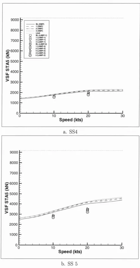
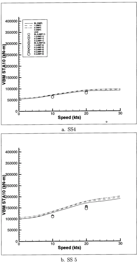
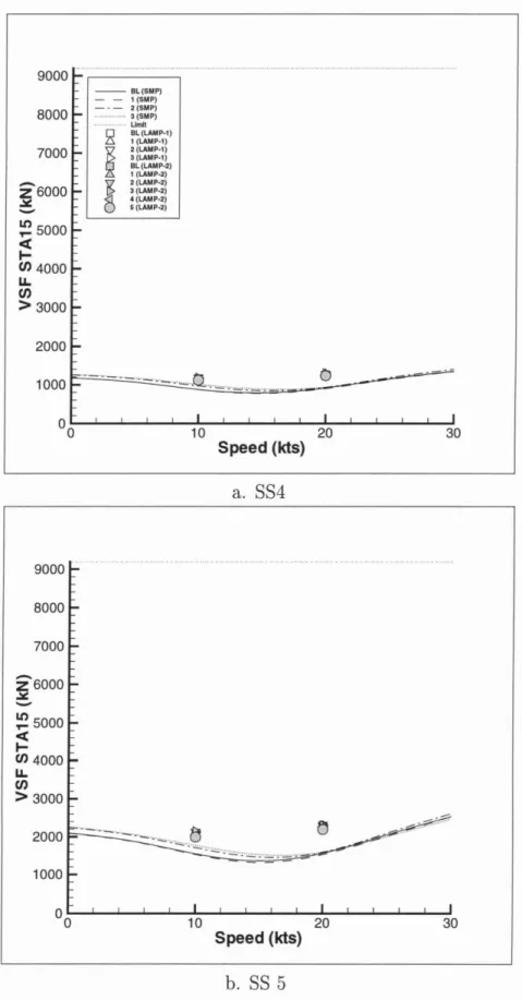
are then applied. In the first method, LAMP is used to simulate irregular seas runs of about fifteen minutes real time each. Motion and load amplitudes are then calculated directly from the LAMP time domain predictions. In the second method, LAMP is used as a regular wave test facility. For heave, pitch, and vertical loads, the ampli-tudes of the first and any higher harmonics are calculated from the regular seas time domain predictions. These harmonics are then used as a form of Response Amplitude Operator (RAO) to predict responses in irregular seas. As mentioned previously, the testing included only head seas. Although much work needs to be done assessing the oblique seas design capabilities of LAMP, time restrictions limited this study to head seas, and vertical motions and loads. However, this is appropriate to an analysis of 3-D time domain code utility in early design, since head seas are often the most severe encountered by a ship, and are typically the subject of experimental tests. Table 2.4 on the next page lists the ship responses which are measured with both SMP and LAMP. This list includes the motions defining the naval and commercial transit limits, and those motions considered by the Bales and McCreight parametric indices. Vertical shear, which typically reaches absolute maxima at the hull quarter points, and vertical bending moment at amidships are compared for the loads.

Heaver Pitcht

Heave Acceleration

Vertical Acceleration at Station 0 Vertical Acceleration at Station 3 Vertical Displacement at Station 20 Relative Motion at Station 0

Relative Motion at Station 3 Relative Velocity at Station 3 Relative Motion at Station 20 Deck Wetness at Station 0 Slamming at Station 3

Propeller Emmersion at Station 20 Vertical Shear Force at Station 5t *

Vertical Shear Force at Station 15t *

Vertical Bending Moment at Station lOt

tOnly these responses are calculated in regular waves.

*

Measured at Sta. 4 & 16 for VLCC, point of static hog maxima. Table 2.4: Measured Responses in LAMP and SMP

Chapter

3

Hull Geometries

3.1

Mathematically Defined Hulls

3.1.1

Motivation

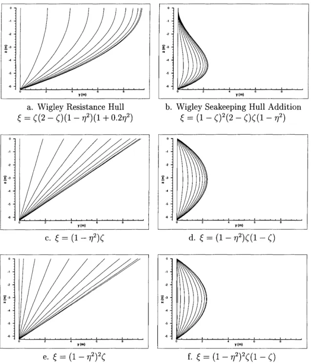
The primary test hulls for this research are a group of six mathematically generated surfaces, derived from the well-known Wigley Seakeeping Hull (hereafter, the Wigley Hull). The Wigley Hull is an extremely simple hull with zero flare along its length. The hull is fore-and-aft symmetric, with offsets becoming zero at the perpendiculars. There is no flat of bottom, and both the stem and stern are vertical. The mathemati-cal definition can be applied to any desired length, beam, and draft. The formulation of the Wigley Hull is fully described in Section 3.1.3. The hull is the baseline for this study, and a plot of the geometry (applied to the study dimensions) is shown in Figure 3-3a, in Section 3.1.4. The baseline has varying depth, which is also discussed in that section.

This hull has proven extremely popular for hydrodynamic research both because of its simplicity and because the hull definition may be included analytically in the governing equations of motion. But why include such a hull in current numerical seakeeping studies, when high power computers are available? The primary reason is again that the hull's simplicity makes it an excellent tool for early code validation. However, though such a hull form is extremely useful for 2-D linear predictions of

seakeeping motions, it is inadequate for proper testing of 3-D nonlinear codes. The alternative is to create a hull which maintains the simplicity of the original Wigley Hull, but which is useful for comparative studies using LAMP and SMP. The hulls designed for this study meet this goal. These mathematically defined hulls were accomplished through the superposition of additional hull forms with the original Wigley Seakeeping Hull components. The use of such hull forms allows the varia-tion of certain hull geometrical parameters which are considered significant in their effect on both seakeeping and other hydrodynamic characteristics, such as resistance. Additional advantages and disadvantages of such hull forms include:

• With proper variation of mathematical components, desired hull characteristics may be easily achieved, without possibly inconsistent modifications of offset or B-Spline definitions.

• Simple hull shape eliminates many hull characteristics which might reduce the applicability of the research. Specifically, fore-and-aft symmetry removes ef-fect of stern shape as a variable. However, some of these simplifications may simultaneously reduce the realism of the tests.

• Significant research has previously been conducted on Wigley type hulls, for example, Gerritsma (1988), Journee (1992), and Adegeest (1994) [24, 25, 26].

• Mathematical definition allows rapid generation of panelized hulls.

Section 3.1.2 further describes the selection of which parameters were to be held constant or varied for each hull. The mathematical hulls are to act as the "naval-like" hulls in this study, although the final choice of hull particulars certainly does not preclude commercial applicability.

3.1.2

Constant and Varied Hull Parameters

Before commencing the design of the mathematical hull forms, the possible combina-tions of hull parameters which would be used to specify the hull shape were examined. Priorities in proper selection of the parameters were:

1. Select standard hull parameters generally used by naval architects in describing hull shape characteristics.

2. Vary items which are accepted as having a significant impact on the hydrody-namic characteristics of ships.

3. Vary items which would realistically be possible to alter in the early design stages of a ship hull.

4. Hold constant parameters which would potentially be constrained by the spec-ifications of a design, such as length, beam, draft, and displacement.

5. Limit geometry variation to isolate changes in hydrodynamic performance to a small number of variables.

6. Vary parameters to develop a hull form which includes characteristics that do not affect linear seakeeping calculations (especially above waterline hull form.)

7. Vary the proper number of parameters to constrain the hull selection uniquely without preventing a determinate solution. This is a function of the number of mathematical hull forms to be superimposed.

It is generally accepted that overall seakeeping performance may be improved by anyone of several methods [11, 12]: increasing length to draft ratio (LIT), increasing the ratio L2_{I (BT), increasing the beam to draft ratio, BIT (which increases damping}

effects), and increasing length to volume ratio

(LI"V).

Besides these primary ratios, seakeeping may also be improved by altering the standard coefficients of form, espe-cially by reducing block coefficient (CB) or increasing waterplane coefficient (C_wp ).

It is also possible to alter longitudinal bending moment responses by varying the midships section coefficient (C

M) .

While the above adjustments can in general improve seakeeping motions, it is possible to specifically improve pitch response by increasing waterplane area at the ends of the ship - and particularly the bow. Quantitatively, this requires increasing the waterplane moment of inertia coefficient, CA. At the bow, which controls worst case

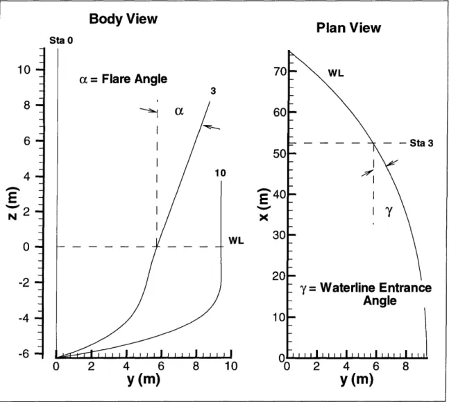
pitch response in head seas, waterplane area may be maximized by increasing both the flare angle (a) and/or the waterplane entrance angle (7). These two angles are defined in Figure 3-1 on the facing page. Increasing flare forward will generally result in a more "V-shaped" hull form. Flare angle may usually be increased to 20-25°, and a reasonable hull form maintained [11]. In fact, U.S. Navy design recommendations, based on work conducted by Bales (1979), state that ships in this range of flarel have "superior wetness" performance [27, 28]. The flare for the first set of varied hulls was in fact set at 20°. Increasing entrance angle will also improve pitch response, but can have a drastic effect on ship resistance. These angles, and flare in particular, will to a great extent determine the hull shape near the bow. Proper flare can reduce pitch motions, green water on deck, and relative bow motions. Extreme flare can in turn create severe slamming loads.

Once the important hull parameters in seakeeping prediction were defined, the task of choosing which to vary and which to maintain constant was completed. Because of their significant impact on hydrodynamic performance, flare and entrance angle were chosen as the primary parameters to be varied in generation of a test series. Length, beam, draft, and displacement are held constant. Hull depth, although not a factor in the mathematical definition, is constant for all variants. These restrictions simulate a realistic challenge in early design. Ship payload and performance requirements may drive the choice of main particulars, but the designer has some latitude in creating a hull form (e.g. in selection of flare and entrance) that meets these criteria.

3.1.3

Hull Component Definitions

With the selection of hull parameters to be varied or maintained constant, the actual task of mathematical definition is possible. Achieving reasonable mathematical hull forms proved quite challenging, and is completely documented in Moton (1996) [29]. A review of the process and the final definition method is included here. All hulls are defined with nondimensional coordinates, since the final dimensions were not chosen

Body

View

Plan View

Sta 0 10

a

=

Flare Angle 3 8 ~

a

I 6 _I - - Sta 3 I 4 I 10

...--.

I

E

--""'2 I

_Y

N I 0 - - -

- -

WL -2 _'Y

₌

Waterline Entrance Angle -4 -6 0 2 4 6 8 10 2 4 6 8

y(m)

y(m)

Figure 3-1: Flare and Entrance Angle Definitions (Variant 3 Lines)

until after the mathematical definition was created. These coordinates are:

TJ = 2x/L

~

=

2y/B

(= 1

+

z/T

with x

=

a

at amidships, and positive forward; y

=

a

on the centerline and positive to port; and z =

a

at the design waterline and positive up.