Analysis of Functionally Graded Material Object
Representation Methods
by
Todd Robert Jackson
B.S.E., Princeton University (1994)
S.M., Massachusetts Institute of Technology (1997)
Submitted to the Department of Ocean Engineering
in partial fulfillment of the requirements for the degree of
Doctor of Philosophy
at the
MASSACHUSETTS INSTITUTE OF TECHNOLOGY
June 2000
©
Massachusetts Institute of Technology 2000. All rights reserved.
Author...
..
..
..
..
...
...
. -. . .. ..-. :.-.. . . .. .. . . . .. . . . .. .. .. . ...Department of Ocean Engineering
January 28, 2000
Certified by...
Certified by...
Are iitorl 1
Nicholas M. Patrikalakis, Ph.D.
Kawasaki Professor of Engineering
,jJ ,,isSupervisor
..
. ...
....
*.
. .*
-
. . . .*
Emanuel M. Sachs, Ph.D.
Professor of Mechanical Engineering
Thesis Supervisor
Nicholas M. Patrikalakis
Chairman, Departmental Committee on Graduate Studies
MASSACHUSETTS INSTITUTE OF TECHNOLOGY
Analysis of Functionally Graded Material Object Representation
Methods
by
Todd Robert Jackson
Submitted to the Department of Ocean Engineering on January 28, 2000, in partial fulfillment of the
requirements for the degree of Doctor of Philosophy
Abstract
Solid Freeform Fabrication (SFF) processes have demonstrated the ability to produce parts with locally controlled composition. To exploit this potential, methods to represent and exchange parts with varying local composition need to be proposed and evaluated. In modeling such parts efficiently, any such method should provide a concise and accurate description of all of the relevant information about the part with minimal cost in terms of storage. To address these issues, several approaches to modeling Functionally Graded Material (FGM) objects are evaluated based on their memory requirements.
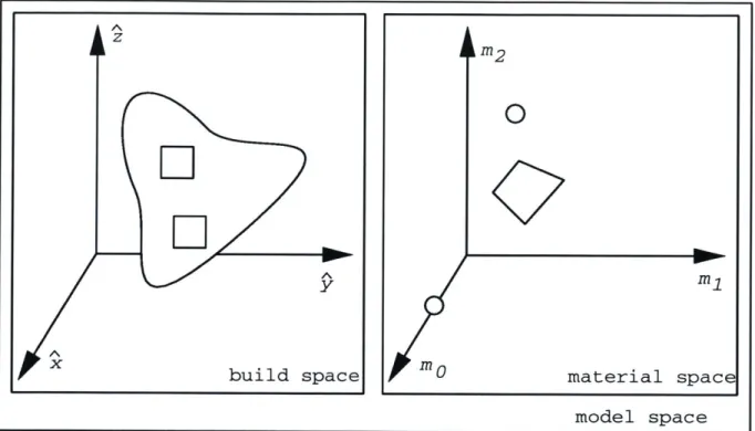
Through this research, an information pathway for processing FGM objects based on image processing is proposed. This pathway establishes a clear separation between design of FGM objects, their processing, and their fabrication. Similar to how an image is represented by a continuous vector valued function of the intensity of the primary colors over a two-dimensional space, an FGM object is represented by a vector valued function spanning a Material Space, defined over the three-dimensional Build Space. Therefore, the Model Space for FGM objects consists of a Build Space and a Material Space. The task of modeling and designing an FGM object, therefore, is simply to accurately represent the function m(x) where x E Build Space.
Data structures for representing FGM objects are then described and analyzed, including a voxel-based structure, finite element method, and the extension of the Radial-Edge and Cell-Tuple-Graph data structures with FGMDomains in order to represent spatially varying properties. All of the methods are capable of defining the function m(x) but each does so in a different way. Along with introducing each data structure, the storage cost for each is derived in terms of the number of instances of each of its fundamental classes required to represent an object.
In order to determine the optimal data structure to model FGM objects, the storage cost associ-ated with each data structure for representing several hypothetical models is calculassoci-ated. Although these models are simple in nature, their curved geometries and regions of both piece-wise constant and non-linearly graded compositions reflect the features expected to be found in real applications. In each case, the generalized cellular methods are found to be optimal, accurately representing the intended design.
Thesis Supervisor: Nicholas M. Patrikalakis, Ph.D. Title: Kawasaki Professor of Engineering
Thesis Supervisor: Emanuel M. Sachs, Ph.D. Title: Professor of Mechanical Engineering
Dedication
This dissertation is dedicated to my wife, Courtney, and our families. Thank you for your unwaiver-ing love and support as I pursued my dream.
Acknowledgements
I wish to thank my thesis supervisors, Professors Nicholas M. Patrikalakis and Emanuel M.
Sachs, for the opportunity to participate in this research project. Participating in a project forging new grounds in Computer Aided Design and Manufacturing has been an exciting, challenging, and rewarding process. I am grateful for their mentoring and patience as we explored new ideas together and defined the direction of my research. Professor Michael J. Cima also deserves recognition for his role in helping to define the direction of this work. I would also like to thank and recognize the efforts of my colleagues who contributed invaluable energy and insights to the challenges presented through this work, including David Brancazio, Dr. Wonjoon Cho, Hongye Liu, and Dr.
Hauijun Wu. Along with my thesis supervisors, Dr. Cho's critical readings of the drafts of this
manuscript have been instrumental in expediting the completion of this document and ensuring that the final draft meets the expectations for an MIT dissertation.
The author and investigators in this project also gratefully recognize the financial support of the
National Science Foundation (grant #DM19617750) and the Office of Naval Research (grant #N00014-96-1-000857), without which this research would not have been possible.
The examples used in this thesis were generated through the CAD system SolidWorks and meshed using the Finite Element Analysis package Algor.
Finally, I wish to thank my friends and colleagues for their friendship and support through my years at MIT. The names are too numerous to mention here, but their comradery deserves just as much acknowledgement. Please forgive me for not attempting to list names here, for to do so would inevitably lead to the omission of someone who should not have been excluded. I choose rather to close these acknowledgements with a simple "thank you" and trust they all will realize how much their friendships mean to me and take some satisfaction in seeing this work in final form.
Contents
1
Introduction 1.1 M otivation . . . . 1.2 Scope of research .... ... 1.2.1 T hesis . . . . 1.2.2 Approach . . . .1.3 Solid Freeform Fabrication . . . .
1.3.1 Single material SFF processing . . . .
1.3.2 Local Composition Control through SFF with
1.3.3 Modeling and processing for SFF . . . . 2 Previous work
2.1 Introduction . . . . 2.2 Current data exchange methods . . . . 2.2.1 ST L file . . . .
2.2.2 STEP: STandard for the Exchange of Product
multiple
model
2.3 Modeling of FGM objects . . . . 2.3.1 Voxel-based modeling . . . . .
2.3.2 Finite element modeling . . . . 2.3.3 Generalized modeling methods 2.4 Discussion . . . .
3 Identification of issues in FGM modeling 3.1 M otivation . . . . 3.2 Modeling shape versus shape and composition 3.2.1 Geometric modeling . . . .
3.2.2 Geometric and material modeling .. 3.3 Accuracy in representation . . . . 3.3.1 Shape . . . . materials data 21 21 21 21 22 23 23 24 24 28 28 28 29 31 33 33 37 37 40 42 42 42 42 43 46 46 . . . . . . . . . . . . . . . . . . . .
3.3.2 M aterial . . . . 3.4 Processing FGM models for fabrication.
3.4.1 Image processing . . . . 3.4.2 FGM model processing . . . . . 3.5 Discussion . . . .
4 Modeling composition through decomposition
4.1 M otivation . . . .
4.2 Nomenclature . . . . 4.3 Voxel-based modeling . . . . 4.4 Triangulated shells . . . . 4.5 Finite element meshes . . . . 4.6 Generalized cellular decomposition or multi-region B-rep . 4.6.1 Data structures for topology . . . . 4.6.2 FGMDomains . . . . 4.6.3 Relationship between FGMDomains and topology 4.7 D iscussion . . . .
5 Bounds for voxel-based model growth 5.1 M otivation . . . .
5.2 Voxel size dictates lattice size . . . .
5.3 Geometric constraint on voxel size . . . .
5.4 Composition constraint on volume fraction
5.5 Composition constraint on voxel size . . . 5.5.1 Constraint based on discontinuities
5.5.2 Constraint based on gradient . . . 5.6 Discussion . . . .
resolution . . .
in composition
6 Bounds for meshed model growth
6.1 M otivation . . . . 6.2 Curve meshing . . . .
6.2.1 Approximating a circular arc . . . .
6.2.2 Approximating a G1 curve . . . .
6.2.3 Approximating an arbitrary curve or curves
6.3 Surface meshing . . . . 6.3.1 Approximating the surface of a sphere . . . 6.3.2 Approximating an arbitrary surface patch .
91 91 91 92 95 97 97 101 104 110 . . . 1 10 . . . 1 10 . . . 1 1 1 . . . 1 12 . . . 1 16 . . . 1 1 7 . . . 1 1 7 119 . . . . 4 7 . . . . 4 8 . . . . 5 0 . . . . 5 3 54 54 55 56 58 60 64 65 76 85 87 47
6.4 Volume meshing ... ...
6.4.1 Bounds on the number of tetrahedra due to geometric accuracy . . 6.4.2 M aterial curvature . . . . 6.4.3 Bounds on number of tetrahedra due to composition accuracy . . .
6.5 Relationship between the number of triangles and nodes in a triangulated shell 6.6 Relationship between the number of
tetrahedra and nodes in a finite element mesh
6.7 D iscussion . . . . 7 Approaches to FGM design
7.1 M otivation . . . . 7.2 FGM fitting . . . . 7.3 FGM library . . . .
7.4 FGM chamfer, fillet, and blending . . . .
7.5 D iscussion . . . .
8 The cost of representing composition 8.1 M otivation . . . . 8.2 Case studies . . . .
8.2.1 Sphere of unit radius . . . .
8.2.2 Bar with graded transition .
8.2.3 Graded composition from boundary 8.2.4 Cylinder butted to plate . . . .
8.2.5 Drug delivery device . . . .
8.2.6 Widget Mold . . . .
8.3 Discussion . . . .
9 Conclusions and Recommendations 9.1 Conclusions . . . .
9.2 Contributions . . . . 9.3 Future work and recommendations
9.3.1 Investigation into generalized
9.3.2 Exploration of FGMDomains
9.3.3 FGM object design methods
9.3.4 Establishment of a design me
9.3.5 Tools for fabricating FGM ob
of cavity in block
FGM.mdele... FGM modeler . . . .
hodology for FGM
objects
.jects . . . .
9.3.6 Efficient methods for voxel-based and finite element models . . . .
. . . . . . . . 120 121 121 124 126 128 129 133 133 133 145 146 149 150 150 151 151 158 166 179 189 198 208 209 209 212 213 213 213 213 214 215 215 t
9.3.7 Exploration of material systems . . . 215
9.3.8 Exploration of halftoning strategies . . . . 216 9.3.9 Exploration of Design Rules . . . 216
List of Tables
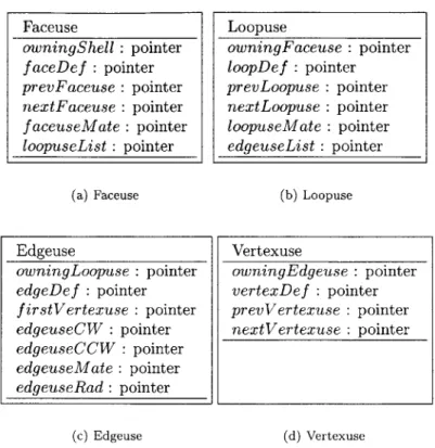
4.1 Storage costs for each instance of each class within the Radial-Edge data structure. 70
4.2 Storage costs for different objects within the Cell-Tuple Data structure. . . . . 76
4.3 Storage costs of FGMDomain definitions used in analysis of memory requirements for generalized FGM modeling methods. . . . . 85
4.4 The relationships between the number of topological entities in Radial-Edge data structure and each derived class of FGMDomain. . . . . 87
4.5 The relationships between the number roles of each topological entities in Radial-Edge data structure and each derived class of FGMDomain. . . . . 87
4.6 The relationships between the number instances of each class in the Cell-Tuple-Graph data structure and each derived class of FGMDomain. . . . . 88
4.7 Memory requirements for Exhaustive Enumeration, Triangulated B-Rep, Tetrehedral Mesh, Radial-Edge, and Cell-Tuple-Graph solid modeling methods. . . . . 90 6.1 Modification to triangulated mesh. . . . 126
8.1 Storage costs associated with primitive data types on a Silicon Graphics 02 worksta-tion with 64 bit processor. . . . 151
8.2 FGMDomain and Cell-Tuple-Graph objects required to represent sphere object
ex-actly and the associated storage cost. . . . 155
8.3 Number of instances of Radial-Edge objects required to represent sphere model exactly
and the associated storage cost. . . . 155 8.4 FGMDomain and Cell-Tuple-Graph objects required to represent bar object exactly
and the associated storage cost. . . . 164
8.5 The Radial-Edge objects required to represent FGM bar object exactly and the asso-ciated storage cost. . . . 164
8.6 FGMDomain and Cell-Tuple-Graph objects required to represent FGM
8.7 Radial-Edge objects required to represent FGM block-with-cavity object exactly and
the associated storage cost. . . . 176
8.8 FGMDomain and Cell-Tuple-Graph objects required to represent FGM cylinder-plate
object exactly and the associated storage cost. . . . 185 8.9 Radial-Edge objects required to represent FGM cylinder-plate object exactly and the
associated storage cost. . . . 186 8.10 Cell-Tuple-Graph objects required to represent FGM drug delivery device object
ex-actly and the associated storage cost. . . . 195
8.11 Radial-Edge objects required to represent the topology of FGM drug delivery device
object exactly and the associated storage cost. . . . 196
8.12 FGMDomain and Cell-Tuple-Graph objects required to represent FGM Widget Mold
exactly and the associated storage cost. . . . 204
8.13 Radial-Edge objects required to represent the topology of FGM Widget Mold exactly
List of Figures
1-1 (a) 3D Printing illustrating how SFF processes can build a part on a point-wise basis.
(b) Parts fabrication through 3D Printing demonstrating the flexibility of SFF to
produce complex geometries. [59] . . . . 25
1-2 3D Printing illustrating Local Composition Control by selectively depositing droplets of different material into a powderbed to form a Functionally Graded Material object. 26
1-3 Information flow for 3D Printing. . . . . 26
2-1 STL file format. The boundary of a model is described as a list of triangular facets and their norm als. . . . . 30
2-2 (a) Faceted approximation of a wheel (26906 triangles). (b) STL text file describing part (3.17 Megabytes in ASCII format, 1.34 Megabytes in binary format) . . . . 31 2-3 The structure of STEP. . . . . 32
2-4 (a) Geometric and (b) topological entities defined with Part 42 of STEP (IS010303). 34
2-5 (a) Surfaces defining the boundary of a wheel (269 surfaces). (b) STEP encoding of
the part (11.1 M egabytes). . . . . 35 2-6 Photograph of actual brain, magnetic resonance imaging of brain, voxelized model
of brain. (image courtesy of University of Washington Structural Informatics Group http://sig.biostr.washington.edu/) [77] . . . . 36 2-7 (a) Proposed decomposition of solid model into atlases. (b) Proposed data structure
for rm-object modeling based [40]. . . . . 38 2-8 (a) Model motivating need for representation method for heterogeneous objects with
rm-sets [40]. (b) Example of a graded bar represented as an rmn-object, decomposed into cells [40]. . . . . 39 2-9 (a) A pulley consisting of graded material defined as a cellular model with Bezier
triangles and tetrahedra. (b) A drug delivery device defined as a cellular model with B6zier triangles and tetrahedra. [33, 32]. . . . . 40
3-1 (a) The Model Space represented by state-of-the-art solid modeling systems. (b) Associating of materials to regions within a model. . . . . 44
3-2 The Model Space for objects consisting of graded material spans both the Build Space
(X) and a Material Space (M) in which the material variations are defined. . . . . . 45
3-3 To define an FGM object, each point in the Build Space (x E X) must map to a
composition in the Material Space (m(x)
C
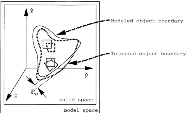
M) . . . . 45 3-4 The maximum distance between the intended object's boundary and the modeledboundary is the geometric accuracy (6g) of the modeled object.) . . . . 47
3-5 Visual interpretation of material accuracy, showing the difference between the desired
composition m*(xo) and the modeled composition m(xo) at the point x0 in Build
Space. ... ... 48
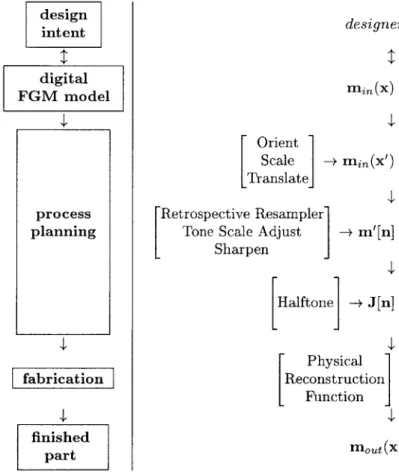
3-6 Steps of the information flow for image processing. . . . . 49
3-7 (a) Initial image: Ii,(x). (b) Sampled image: I'(n). (c) Halftoned image: J(n). (d)
Physically reconstructed image: It(x). . . . . 51 3-8 Steps of the information flow for FGM model processing . . . . 52
4-1 Model consisting of two tetrahedra used to illustrate various modeling methods. Shown is the wireframe of the model. . . . . 55
4-2 Relationships between classes in an exhaustive enumeration method for modeling
FG M objects. . . . . 57
4-3 (a) Voxelized representation of sample model. (b) VoxelModel object model. . . . . . 57
4-4 Relationships between classes in the triangulated boundary representation approach for modeling FGM objects. . . . . 58
4-5 (a) Triangulated shell representation of sample model. (b) Object model showing the instances data required to represent the sample model in the data structure. . .. .. 59
4-6 Relationships between classes in tetrahedral mesh approach to modeling FGM objects. 61 4-7 (a) Tetrahedron classes for consideration in meshed modeling representations. (b)
Vertex classes for consideration in meshed modeling representations. . . . . 61
4-8 (a) Tetrahedral mesh representation of sample model. (b) Object model showing the instances data required to represent the sample model in the data structure. .. .. 62
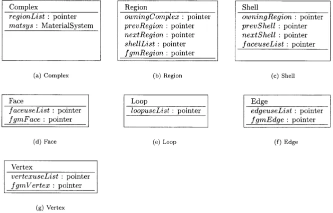
4-9 The classes comprising the Radial-Edge data structure and how they are related. . . 66
4-10 Topological classes defined within the Radial-Edge data structure and their attributes. 67 4-11 The Uses of topological entities within the Radial-Edge data structure. . . . . 69
4-12 (a) Radial Edge representation of sample model. (b) Object model showing the in-stances of topological entities required to represent the sample model in the Radial Edgedata structure. ... ... 71
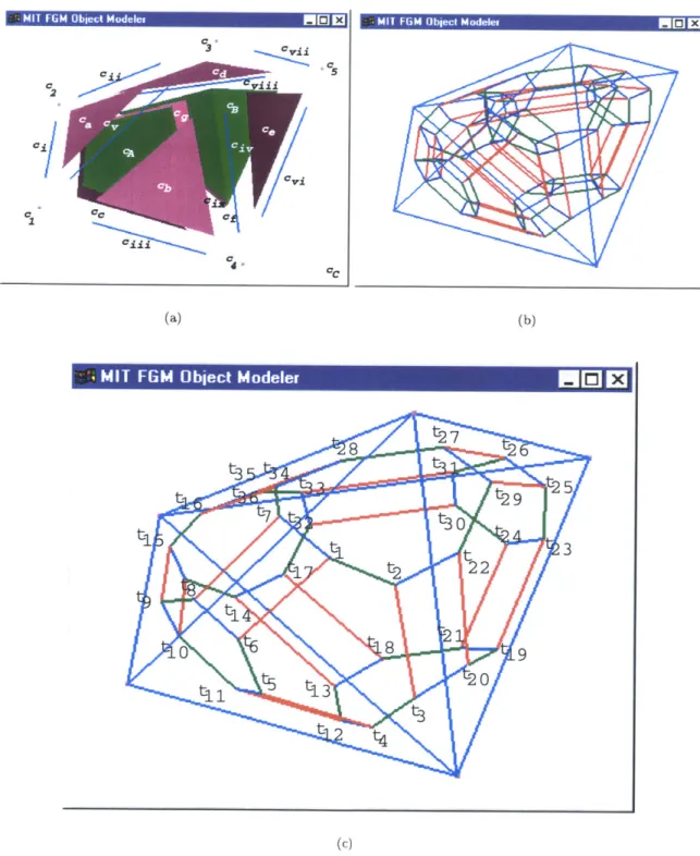
4-13 (a) Cells in model. (b) Graph of tuples. Paths between tuples are colored according to dimension: red=0, green = 1, blue = 2, dashed blue/yellow = 3. (c) Graph of
tuples over boundary with each tuple labelled. . . . . 73
4-14 Relationships between classes in Cell-Tuple-Graph data structure. . . . . 74 4-15 Illustration of switch operator performed on tuple ti for dimension 1 (green). (a)
Cells in tuple ti. (b) Location of tuple ti in graph. (c) Cells in Tuple t2. (d) Location
of tuple t2 in graph. . . . . 75
4-16 Zero dimensional FGMDomain. . . . . 77
4-17 One dimensional FGMDomain: FGMRationalBezierCrv. . . . . 78
4-18 Two dimensional FGMDomains: FGMRationalB6zierTri, FGMRationalBezierQuad, and FGM PlanarSurface. . . . . 79
4-19 Three dimensional FGMDomains: FGMRationalBezierTet, FGMRationalB6zierPent, FGMRationalBezierHex, and FGMBRepRegion. . . . . 82
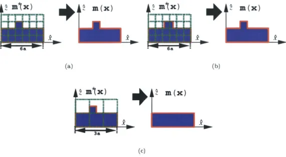
4-20 (a) Modeling two piecewise constant regions with composition information associated with (a) the two regions and (b) the vertices. In order to represent two piece-wise constant regions when the material information is associated with the vertices, the interface region must be meshed as in (c). . . . . 89 5-1 (a) The addition of a feature to a voxel-based data structure. (b) Modified voxel-based
model to capture intended feature. . . . . 92 5-2 Examples of distretization of the intended boundaries of models into voxels. . . . . . 93 5-3 Intended designs for object boundary (m*(x)) and modeled boundary (m(x)). The
dimensions of the voxels are 6,
y,
6z = a. (a.) Boundary of geometric feature lies along voxel boundaries. (b.) Boundary of geometric feature lies off voxel boundaries but is still captured in representation. (c.) Voxel mesh is too coarse to capture geom etric feature. . . . . 955-4 Thresholding of continuous grading to discrete levels maintained in voxel representa-tion (a) nA = 2, (b) (a) nx = 3, (b) (a) nA = 4, (d) nA = 7. . . . . 96 5-5 Examples of discontinuities in composition. (a) Discontinuity between two regions of
uniform composition. (b) Discontinuity with regions of graded composition. . . . . . 97 5-6 (a) Voxel to approximate a subregion of discontinuous composition. The discontinuity
in composition occurs of the plane ir. (b) The desired composition (m*(x)) over the subregion occupied by the voxel. . . . . 98 5-7 Thresholding of designed material assigned to discretized regions of uniform
5-8 Intended designs for material distribution (m* (x)) and modeled compositions (m(x)). 6, 6Y, 6Z = a (a.) Boundary of material feature lies along voxel boundaries. (b.) Boundary of material feature lies off voxel boundaries but is still captured in repre-sentation. (c.) Voxel mesh is too coarse to capture material feature. . . . . 100 5-9 (a) Region of linearly graded material and direction ('v) of grading. (b) The desired
graded to be assigned to the region. . . . . 101 5-10 Examples of linearly graded designs thresholded to uniform composition assignments
to voxels. ... ... 102
5-11 Storage cost (in bytes per material) required to represent a model as a function of
normalized Build Space volume (V* = L' ), which is equivalent to the number of voxels (n,,,). (slope = bytes) . . . . 106 5-12 Storage cost (in bytes per material ) required to represent a model as a function of
Build Space volume (V in m3
) for an SFF process with a resolution of 6. = 6y = 6Z= 10-4m. (slope = 1.25 x 10¹¹"Q.) . . . . 107 5-13 Storage cost (in bytes per material ) required to represent a Build Space with a
cross-sectional area of L. x LY = 10- 2m2 as a function of Build Space height (L,), for an
SFF process with a resolution of 6, 3z = 6Y = = 10-'m (slope = 1.25 x 1 09 byes
)
1086-1 Error associated with approximating a circular arc with a straight line segment.. . 111 6-2 The maximum arclength of a circular arc (As) that can be approximated by a single
line segment within a prescribed accuracy (cg), plotted as a function of 69-. The actual, maximum arclength that can be approximated by a single line is also plotted. . . . . 113 6-3 Convergence to the shape of the arc with an increasing number of straight line
seg-ments: (a) nsegments = 1, (b) nsegments = 2, and (c) nsegments = 4. .. .. . . . . 114
6-4 The number of line segments required to approximate a circular arc of unit arclength, plotted as a function f R . . . . 114
g
6-5 (a) An arbitrary tangent continuous curve. (b) Approximation of a tangent continuous
curve with a chain of line segments. . . . . 115 6-6 (a) An arbitrary curve. (b) Approximation of an arbitrary curve with a chain of line
segm ents. . . . . 117 6-7 (a) A triangle approximating a patch of a sphere's boundary. (b) Enlarged view of
triangle showing the circumscribed circle and the approximation error. (c) Approxi-mation of circular arc of radius R with a line segment of length D. . . . 118
6-8 Number of triangles required to mesh a sphere to achieve a prescribed approximation accuracy. The data was generated from the STL export module in SolidWorksTM. . 120
6-9 (a) Hypothetical cube of graded material. (b) Parametric line p(u) through the graded material. (c) Hypothetical variations of the volume fractions of the different materials along the curve p(u). . . . 123
6-10 (a) Minimum material feature size determined by the minimum dimension of an
inter-nal feature of uniform composition. (b) Minimum material feature size determined by the minimum distance of the object's boundary and an internal feature of the uniform composition. (c) Minimum material feature determined by the distance between two discontinuities in material variation. . . . . 124
6-11 Topological operations for modifying a closed, triangulated shell. (a) The subdivision
of a face into three triangles (Opi). (b) The subdivision of an edge into two edges (Op"i). (c) The creation of a hole through the shell (Opinr). . . . . 127 6-12 Methods to modify a tetrahedron with the addition of a new node. . . . . 128 7-1 (a) Set of data points. (b) Surface fit of data points. . . . . 134
7-2 Illustration of evaluation of distance from features (red) to node points (black) and
the offset region (yellow) in which the composition is to be fitted. . . . . 135 7-3 Grading styles for the design of FGM objects as a function of distance: (a) uniform,
(b) linear, (c) and (d) quadratic, and (e) cubic. . . . . 136
7-4 (a) Fit of composition (smoothly blended at re) designed as a quadratic function of distance within a unit cube from point po = (0,0,0) (r, =
Ocm,
r, =}cm,
mS = [0 1 01T, me = [1 0 O]T). (b) Rendering of nodes colored according to composition.(c) Rendering of material variation over slices through cube. . . . . 138 7-5 (a) Previous design plus fit of composition (smoothly blended at r, =
}cm
and re1cm) designed as a cubic function of distance within a block from point po = (0,0,0)
(M = [1 0 O]T, me = [0 0 1]T). A uniform composition of m = [0 0 I]T is assigned to all nodes beyond a distance of 1 mm from point po = (0,0,0). (b) Rendering of nodes colored according to composition. (c) Rendering of material variation over slices through cube. ... ... 139 7-6 (a) View of solid cube with composition designed as a cubic function of distance within
a unit cube as from the line passing through po = (0, 0,0) to pi = (1, 1,1) (rs =
0cm,
re = 1cm, m. = [1 0]T, m - [0 I]T). (b) View of nodes in mesh. (c) View of slices
through FGM cube. . . . . 140
7-7 Fit of composition designed as a linear function of distance within a unit cube from
plane 7r : z = 0 (r, = 0cm, re = 1cm, m, = [1 O]T and me = [0 1]T. (a) View of solid cube. (b) View of nodes in mesh. (c) View of slices through FGM cube. . . . . 141
7-8 (a) Design of tool on commerical CAD system. The dimension of the tools is 100mm x
50mm x 10mm. (b) Phantom view of the tool showing internal features (cooling
channels). ... ... 142
7-9 (a) Fit of nodes to intended composition (smoothly blended at re) designed as a quadratic function of distance from the boundary of the tool (r, =
Omm,
re = 1mm). (b) View of composition grading over slices through FGM model. . . . . 1437-10 Fit of composition (smoothly blended at re) designed as a quadratic function of dis-tance from a subset of the boundary of a tool (r, =
Omm,
re = 5mm ). The dimension of the tool is 100mm x662mm x20 mm. (a) View of solid tool. (b) View of nodes in mesh. (c) View of slices through FGM model. . . . . 1447-11 (a) A texture primitive stored in a feature library. (b) The mapping of the feature over a plate. (c) The mapping of the feature over a torus. . . . . 145
7-12 (a) Primitive of regions containing drug. (b) The initial pill consisting of a uniform base material. (c) The mapping of drug primitives into the drug delivery device. The placement of of the primitives tailors the drug release profile. . . . . 146
7-13 (a) Original design of corner of part. (b) Chamfered corner. (c) Filleted corner. . . . 147
7-14 (a) Original material distribution over a cross-section of a block. (b) Material distri-bution over block cross-section with material chamfer. . . . . 147
7-15 (a) Original material distribution over a cross-section of a block. (b) Material distri-bution over block cross-section with material fillet. . . . . 148
7-16 (a) Original material distribution over a cross-section of a block. (b) Material distri-bution over block cross-section with material blend . . . . 149
8-1 Geometric design of unit sphere. . . . . 152
8-2 Voxelized approximation of sphere. . . . . 152
8-3 Triangulation of sphere. . . . . 153
8-4 (a) Vertices and edges in generalized representation of sphere. (b) Faces in generalized representation of sphere... ... 154
8-5 Graph of storage cost for representing a unit sphere as a function of geometric accuracy for the data structures considered. . . . . 156
8-6 Graph of storage cost for representing a sphere as a function of geometric accuracy in the STL and STEP file formats. . . . . 157
8-7 Geometric bar specimen to contain smoothly graded transition between two different com positions. . . . . 158
8-8 (a) Desired decomposition of bar into uniform and graded regions. (b) Graded com-position along length of bar. . . . . 159
8-10 Tetrahedral mesh approximation of bar. . . . . 161 8-11 (a) Vertices and edges in generalized representation of bar. (b) Faces and regions in
generalized representation of bar. . . . . 163 8-12 Graph of storage cost for representing an FGM bar specimen as a function of material
accuracy within the indicated data structures with c. =
0.1mm.
. . . . 165 8-13 Geometric design of block with cavity. . . . . 1668-14 (a) Intended density distribution over bar specimen, grading of fully dense material at the surfaces x = 30mm and y = 10mm to 20% density at a distance of 10mm from these boundaries. (b) View of halftoned bar illustrating porous macro-structure generated through the halftoning of the continuous FGM model into binary material prim itives. . . . 167
8-15 (a) Initial compositions of block and the selection of the desired faces from with the
composition will be graded. (b) Desired grading from the selected feature. . . . 169
8-16 Approximation of block geometry with tetrahedra within a finite element mesh. (2206
boundary (external) facets, 8685 tetrahedra, and 2197 nodes) . . . 170
8-17 (a) Nodes of the tetrahedral mesh colored according to their assigned compositions.
View of composition grading assigned to tetrahedral mesh over slices defined by the planes (b) 7r : x = oxffset, (c) 7r : y = Yof fset and (d) 7r : z = Zoffset. . . . . 171
8-18 (a) Wireframe view of block decomposed into FGMDomains. (b) View of block with
FGMDomains colored according to class and degree of shape and material variation. (c) Exploded view of three dimensional FGMDomains, colored according to their degrees of geometric and material variation. . . . . 174
8-19 Graph of storage cost for representing a block (with composition graded from the
boundary of a cavity) as functions of geometric accuracy (a) cm = 0.001, (b)
Em
=0.0056234, (c) Em = 0.17783, and (d) Em = 1. . . . .. . . . . .. . . .. 177 8-20 Graph of storage cost for representing a block (with composition graded from the
boundary of a cavity) as functions of material accuracy (a)
Eg
= 0.001mm, (b)Eg
= 0.00446688mm, (c) 69 = 0.1122mm, and (d) cg = 0.50119mm . . . . 178 8-21 Geometric design of cylinder butted to plate. . . . . 179 8-22 Initial, piece-wise constant compositions assigned to cylinder and plate. . . . . 180 8-23 (a) Selection of the desired face across which composition will be filleted. (b)Decom-position of model into desired piece-wise constant regions and material fillet. . .. . 181
8-24 Voxel-based representation of cylinder and plate. . . . . 182 8-25 Tetrahedral mesh model of cylinder and plate (1708 boundary facets, 7985 tetrahedra,
8-26 (a) Decomposition of cylinder and plate into regions to represent grading exactly
with-in a generalized data structure. (b) Edges and vertices with-in generalized representation of bar butted to plate. . . . 184
8-27 Graph of storage cost for representing a cylinder butted to a plate (with a material
fillet) as functions of geometric accuracy (a) fm = 0.001, (b)
Em
= 0.0056234, (c)m = 0.17783, and (d) Fm = .. . . . 187 8-28 Graph of storage cost for representing a cylinder butted to a plate (with a material
fillet) as functions of material accuracy (a)
E.
= 0.001mm, (b) cq = 0.00446688mm, (c) (9 = 0.1122mm, and (d) eg = 0.50119mm. . . . . 188 8-29 Geometric design of boundary of drug delivery device. . . . . 189 8-30 (a) Library drug primitives with minimum geometric and material feature sizes P.and pm. (b) Placement of drug primitives into drug delivery device. . . . . 191 8-31 Representation of the drug delivery device as a tetrahedral mesh. . . . . 193 8-32 Representation of the drug delivery device as a collection of FGMDomains. Shown are
only the vertices and edges bounding the region of uniform composition, into which the drug primitives are placed. (a) Initial vertices and edges of pill. (b) Vertices and edges of device after the addition of a drug primitive . . . . 194
8-33 Geometric design of Widget Mold. . . . . 198
8-34 (a) Representation of the Widget Mold as a tetrahedral mesh (wireframe view). (a) Representation of the Widget Mold as a tetrahedral mesh (solid view). . . . . 200
8-35 (a) View of the nodes in the tetrahedral mesh. (b) View of the material grading over
slices of a tetrahedral mesh representation of the Widget Mold. (c) View of material evaluated over 60% of each tetrahedron's domain. (d) View of material evaluated over 40% of each tetrahedron's domain. . . . . 201
8-36 (a) FGMDomain vertices and edges into which the Widget Mold is decomposed in a
generalized data structure. (b) A single FGMDomain representing the interior of the Widget Mold in a generalized data structure. . . . 202
8-37 Hierarchy from FGMDomain to FGMProcRegion. . . . 203 8-38 Graph of storage cost for representing the Widget Mold (with composition graded
from the boundary) as functions of geometric accuracy (a) cm = 10', (b)
Em
= 10- 3,(c) cm = 10-1, and (d) Em =1. . . . .. . . . .. . .. .. . . . 205 8-39 Graph of storage cost for representing the Widget Mold (with composition gradedfrom the boundary) as functions of material accuracy (a)
Eg
= 10- 3mm, (b) cgSymbols
[al The ceiling of a; the first integer b equal to or larger than a such that 0 < b - a < 1
La] The floor of a; the first integer b equal to or less than a such that 0 < a - b < 1
AP the area of the surface p.
Go position continuity: no breaks or gaps exist over a G' curve or surface
G1 tangent continuity: the tangent vector for a G' curve varies continuously; the orientation of the tangent plane for a G1 surface varies continuously
G2 curvature continuity: the center of curvature for a G2 curve varies continuously; the principal curvatures for a G2 surface vary continously
MO material continuity: the volume fraction of each material varies continuously over an MO region, lim (m(x) - m(x + Ax)) = 0
Ax-O
M' material derivative continuity: the rate of change of the volume fraction of each material varies continuously within an M1 region,
Vm(x)
is continuous at all points x in an M1 region M a vector or array or composition pointsSa storage cost for an object of type a
SbIn storage cost for a Boolean object
S t storage cost for a float object
Sit storage cost for an integer object S, storage cost for a Material System
Sptr storage cost for a pointer object R radius of curvature
U a vector or arracy of points in parameter space Vq the volume of the region of space q
X a vector or array of points in Build Space
Xnxm multidimensional array of data (mn floats or doubles) b Boolean flag (true or false)
dm number of materials in the Material System; dimension of the Material Space in which the
FGM object exists
m a composition stored in an FGM modeling system; a vector of volume fractions of materials in Material System; the modeled point in Material Space
m* the intended composition to be stored in an FGM modeling system; the intended point in
Material Space
n,\ number of intensity levels represented in a voxel-based data structure (each intensity level maps
to a specific volume fraction of material) u a point in parameter space
x a geometric point in Build Space
E9 accuracy in approximating a desired or ideal geometry Em accuracy in approximating desired or ideal composition
Kg curvature of curve or surface
Km material curvature Vf(x) gradient of f(x) at xo; x=xo
(Of Of Of
Vf(x) Vf()IX=XO =K~
'~ax', 1y'
z
X=X. Vf(x) -9
directional derivative of f(x) at point xo in direction ';(=f(x)-) - (
(Of(x)
Chapter 1
Introduction
1.1
Motivation
With recent advances in Solid Freeform Fabrication (SFF), the ability to fabricate parts with Local Composition Control (LCC) is becoming a reality, opening the door to creating a whole new class of parts with graded compositions. Despite the advanced capabilities of these SFF machines, access to this new technology is limited by how information is represented, exchanged, and processed. Designers need new CAD representations to capture their ideas as models with graded compositions and manufacturers need algorithms capable of converting these models into machine instructions for their fabrication. A method for maintaining this information, however, has not yet been adopted as the preferred solution from the many approaches to representing volumetric data. This presents an obstacle to the exploration of tools for capturing design intent, algorithms for processing models for fabrication, and finally exercising the capabilities of LCC to produce FGM parts and tooling, as each method maintains data differently and follows a different paradigm. One of the major obstacles to choosing a solid modeling method through which to explore modeling FGM objects is the memory required to accurately store information within the model. By investigating the memory requirements for various approaches to representing parts with graded compositions, a decision about which method should be preferred as the basis for the solid modeling of FGM parts can be made.
1.2
Scope of research
1.2.1
Thesis
With recent advances in Solid Freeform Fabrication (SFF) technology to achieve Local Composition Control (LCC), Computer Aided Design (CAD) methods need to extended to truly realize the potential of Functionally Graded Material (FGM) parts and tools. To better understand the CAD
issues involved with modeling FGM objects, this dissertation identifies and compares several likely candidate data structures in terms of how they might represent FGM objects. Through this work, the following hypothesis is examined:
"A memory efficient and accurate approach to modeling FGM objects can be achieved by
extending solid modeling methods currently used for mechanical design. This extension consists of incorporating methods to map from a Build Space to a Material Space into their underlying generalized cellular decomposition or B-rep data structures."
Through the exploration of this hypothesis, the information flow from concept to fabrication is outlined, modeling issues for FGM objects are identified, several alternative approaches to FGM modeling are discussed, and sample FGM objects are presented and their expected storage costs are analyzed in terms of each data structure.
1.2.2
Approach
In order to study the memory required to model FGM objects, this dissertation will begin with an overview of what FGM objects are and how they can be fabricated through SFF processes. Next, a review of methods for model exchange is presented followed by proposed solutions for FGM modeling. The decision for selecting one method over another remains an open question at this point. To answer it, issues concerning the modeling of FGM objects are outlined, including the representation of geometry and composition and how this information should be processed into machine instructions for fabrication through SFF. The accuracy of representation of both the geometry and composition are identified as the relevant parameters in evaluating modeling methods and a clean separation is established between the representation of the object and its processing. To address the issue of representation, data structures for maintaining FGM models are then introduced (voxel-based, triangulated shells, finite element based, and generalized cellular decomposition), along with their memory requirements in terms of the data they maintain. Since several of the modeling methods approximate the designer's intent, a relationship is established between the number of instances of each of their data classes with the accuracy at which the intended geometry and composition is captured. Since working with FGM objects is a new concept, a set of design tools are proposed for defining FGM models as pathways for capturing the designer's intent for material variation. In order to explore the storage costs associated with modeling FGM objects, several hypothetical FGM objects are introduced, using these tools, containing features that a real FGM part might possess (such as curved surfaces and nonlinearly graded compositions). The storage costs associated with representing the objects in each modeling method are analyzed, as functions of accuracy in shape and composition representation. This dissertation then concludes with a recommendation for a preferred solid modeling method based on memory considerations and suggests possible directions
for future research.
1.3
Solid Freeform Fabrication
Solid Freeform Fabrication (SFF) refers to a class of manufacturing processes that build objects in an additive fashion directly from a computer model. While some SFF processes are restricted to building in a single material at a time, most can be adapted to exercise some degree of control over the local composition [17, 35, 57]. Such Local Composition Control (LCC) provides the opportunity to design and create parts with graded composition tailored for specific applications. These graded compositions have become known as Functionally Graded Material (FGM) [20, 80] and refer to the tailored distribution of material within a part designed for optimal performance.
The capability of LCC and fabrication of FGM parts could be utilized by a wide variety of industries. Applications could range from multi-color visualization models to functional parts and tools. For example, the potential to convey additional tissue information through multi-color medical models would increase their usefulness in medical applications such as surgical planning [31]. Not limited to prototyping, SFF processes can also build finished parts and tools. The possibility of incorporating graded compositions could be used in applications requiring the optimization of the mechanical properties of parts and tools at a local scale, potentially reducing distortion due to internal stresses, increasing hardness at points of greatest wear, or resisting failure, for example by locally controlled toughening [80]. The application of FGM compositions to drug delivery devices is even being studied as a means to achieve optimal, controlled release of medicine into a patient [78].
1.3.1
Single material SFF processing
SFF processes build parts by repeatedly adding minute primitives of material according to a
com-puter model until the final object is created [3, 39]. Although there are many variations on this process using different materials and mechanisms for adding material, the underlying philosophy is the same: fabricate an object in an additive fashion directly from a computer model. Some of these SFF processes, each capable of building parts in some additive fashion such as Selective Laser Sintering (SLS) [6], Laminated Object Manufacturing (LOM) [10], Stereolithography (SLA) [34], Shape Deposition Manufacturing [74], Selective Area Laser Deposition (SALD) [35], and 3D Print-ing(3DP) [57]. To illustrate how SFF processes work, the 3D Printing process is explained here.
3D Printing manufactures a part by selectively binding powder together according to a computer
model. The build cycle begins by spreading a layer of powder over the print bed. A print head then traverses the bed, selectively depositing binder 1 over the regions corresponding to the interior
of a slice of the computer model. After the layer is printed, the print bed is lowered and another layer of powder is spread. The process of spreading powder, depositing binder, and lowering the print bed is repeated, as shown in Figure 1-1(a), until the entire volume of the object is printed. At the end of the process, the bound powder becomes the manufactured object, effectively rendering the computer model as a physical object. Post processing steps may also be performed, included sintering and infiltration, in order to increase the density and strength of the object. Currently, metal and ceramic parts are being manufactured through 3D Printing, but the potential exists to build with any material supplied in powder form. A collection of parts manufactured with a single material is pictured in Figure 1-1(b).
1.3.2
Local Composition Control through SFF with multiple materials
Considering that most SFF processes build parts on a point-wise basis, a analogy can be made between how parts are constructed and how images and documents are rendered by the computer on display or hard-copy devices. Following this analogy, the capability to generate mixtures of materials similar to how varying intensities of color are generated through image processing is a logical next step for SFF processes. Through the local control of primitives of different material, the material in a part can be controlled on a local scale, achieving what has become known as Local Composition Control (LCC). Although many SFF processes are capable of achieving LCC, how 3D Printing could achieve it is explained here.
Similar to how an ink-jet printer prints color documents, 3D Printing can achieve LCC with multiple materials. This is accomplished by using a print-head with several jets, as shown in Figure 1-2, each depositing binders and/or slurries 2 of unique material. By varying the pattern in which the jets deposit material on the powder-bed, the material composition can be controlled on the scale of the binder droplets (~ 100pm). Regions of uniform and graded composition can be created in a manner analogous to how continuous tone images are rendered on a hard-copy device from primary colors. With this capability, graded compositions can be designed along with the geometry of the part, tailoring the part's physical properties for a specific purpose or function.
1.3.3
Modeling and processing for SFF
Solid Freeform Fabrication (SFF) processes build parts directly from computer models. These models may originate from sampled volumetric data or solid models of parts designed within a CAD system. The processing of these models for fabrication is unique to each SFF system (depending on the architecture and mechanism of adding material) but the general philosophy can be understood by looking at the information flow for 3D Printing, as shown in Figure 1-3.
2
A solution or colloid without binding properties, used as a transport mechanism for locally adding material to an FGM object.
start
Spread powder Apply binder
remove
Lower print bed F
(a)
(b)
Figure 1-1: (a) 3D Printing illustrating how SFF processes can build a part on a point-wise basis.
(b) Parts fabrication through 3D Printing demonstrating the flexibility of SFF to produce complex
geometries. [59]
t
start Spread powderA
l
Apply binders remove -o *jF inished partFigure 1-2: 3D Printing illustrating Local Composition Control by selectively depositing droplets of different material into a powderbed to form a Functionally Graded Material object.
The process begins with a designer interacting with a CAD system to define the shape of the object. The designer uses tools to modify the geometry of the part and the CAD system provides visual and numerical feedback to the designer about the status of the design. The solid model is represented internally by a proprietary CAD representation, which may be exchanged with other designers and manufacturers using a similar system or translated into a neutral file format (such as
STEP [49, 29] or IGES [27]) for exchange between different systems.
design intent digital solid model process planning fabrication finished part Figure designer
proprietary CAD data structure
Convert boundary into triangles - STL fileo
Orient
Scale - STL file, Translatej
Slice into layers -+ SLC file
Raster layers into passes -+ Raster file Encode into instructions -+ 3DP file
Apply binder according to 3DP file
Bound powder
1-3: Information flow for 3D Printing.
in-structions for the fabrication process. The first step in this process is the conversion of the model from its native representation into a tessellation of triangles approximating its boundary. Next, this tessellated model is oriented, scaled, and positioned in order to ensure its optimal fabrication. Once correctly positioned, the model is sliced into layers of polygons. These polygons are then rasterized into scan lines which are then encoded into instructions for the 3D Printer, indicating where to apply binder as the printhead traverses the printbed.
Although capable of achieving Local Composition Control, the pathway for information flow in current practice does not permit either the definition of FGM objects at the design stage or the conveyance of the material variation downstream to the printer.
Chapter 2
Previous work
2.1
Introduction
Computer Aided Design and Manufacturing methods aim to improve the design process and the quality of the finished process by using computers to represent, design, and evaluate models and from these models, generate plans for their accurate fabrication. Initially, CAD systems were simply used to reproduce traditional drafting tools within the computer, enabling the creation and stor-age of digital engineering drawings. As computers and modeling methods evolved, CAD systems evolved as well, from simply representing engineering drawings to allowing the complete definition and representation of solid parts and assemblies in three dimensions, along with all the relevant man-ufacturing data (surface finish, bill of materials, etc.). Relative to Solid Freeform Fabrication (SFF), the capability of solid modeling has enabled designers to create models and directly manufacture the parts through an SFF process, in a manner analogous to producing hardcopy output directly from a word processing program. One of the next challenges for solid modeling is the representation of graded compositions, or Functionally Graded Material (FGM). With their representation, FGM objects could then be designed and fabricated through SFF processes capable of Local Composition Control (LCC). The current standards for data exchange do not allow this, as explained below in the review of current data exchange methods, providing motivation for research into new model-ing methods. To address this shortcommodel-ing, several solutions for modelmodel-ing FGM parts have been proposed by different groups and are also outlined below.
2.2
Current data exchange methods
Data exchange allows designers to communicate models between each other, the customer, and manufacturers. Although there are as many methods to define an exchange specification as there
are CAD systems, two paths are considered here. The first, the STL file format, is introduced as the accepted specification for model processing within the SFF community. The second, STEP (IS010303), represents a neutral exchange standard proposed by the CAD community at large to enable the complete and exact exchange of model information between various CAD systems.
2.2.1
STL file
In current practice within the SFF community, the processing of models for fabrication is based on the STL file format. This format was introduced in 1987 by the Albert Consulting Group and remains the most common specification for the transfer of models to SFF processing systems [42, 47]. Designers use the tools within a commercial solid modeling system to define a model. Once a model is defined, the boundary of the model is tessellated into a collection of triangular facets, approximating the intended design of the part, and written to a file in the STL format. This file is then used as input to the data processor for generating machine instructions for the part's fabrication. At this point, the model may be oriented, scaled, or support structures added to ensure optimal fabrication. The tessellated model is then sliced into layers and instructions unique to each SFF machine for printing each layer are written to a file. This process of information flow is illustrated in Figure 1-3. To represent a part, the STL format maintains a triangulated representation of the model's boundary. The file is organized as a list of solids, each of which maintains a list of facets defining its boundary, as shown in Figure 2-1. The orientation of the facet is defined by: (1) the ordering of the vertices such that they form a counter clockwise circuit when viewed from outside the solid and (2) the outward pointing normal.
The appeal of the STL file to the SFF community comes from its simplicity. Since the STL file is simply a list of triangles, algorithms to read, write, manipulate, and process models are relatively simple to develop and implement (when compared to generalized boundary representation methods). With the convenience of simplicity, however, comes penalties as well. These penalties can be divided into three general categories: approximation tradeoffs, shortcomings in format definition, and conversion errors [47].
Through the representation of solid models as a triangulated boundary representation within the STL format, curves and curved surfaces are approximated, resulting in a loss of information and accuracy. To provide a higher fidelity representation of a designer's intent for curved objects, more triangles must used, resulting in greater storage cost. Therefore, with the use of a triangulated boundary representation, a tradeoff must be made in the accuracy of representation of the model and the memory required to represent that model.
The definition of the STL format, itself, introduces problems. First, the STL file is unnecessarily verbose, containing redundant data. The orientation of each facet, for instance, is doubly defined by the ordering of its vertices and the associated normal. Second, truncation errors are introduced into
Figure 2-1: STL file format. The boundary of a model is described as a list of triangular facets and their normals.
the representation through the use of single precision floating point numbers. This may result in gaps between facets that cannot be easily detected due to the third problem with the format: lack of topological information. Although the topology, or connectivity, between facets may be inferred, the lack of explicit topology prevents models from being quickly validated as being solids;
ie.
having watertight boundaries. STL models containing gaps and holes may be created and not detected without the costly step of re-deriving all of the neighbor information between triangles [4, 5].The final categories of problems with the STL format are due to conversion from the original solid model into the triangulated representation. During triangulation from the original model into the STL file, any of the following errors may be generated: gaps (open shells) or dangling facets formed, degenerate facets recorded, inconsistent normals assigned, or the topology of the model altered [41, 47, 11]. All of these errors are a function of the accuracy and robustness of the algorithms used to convert the native solid modeling representation with the designer's CAD system into the STL file.
To illustrate the STL format, Figure 2-2(a) shows the tessellated representation of a wheel (with a radius of 269 mm), initially designed with swept, freeform surfaces. Figure 2-2(b) is a truncated description of the part as an STL file. The STL model of the wheel has a total of 26906 triangular facets with a reasonable approximation tolerance, requires 3.17 Megabytes to store the data in ASCII format (1.34 Megabytes as a binary file). The model was created and converted to the STL specification using the commercial CAD system SolidWorks TM
STL File Format solid <name> facet normal h, hy fii
outer loop vertex x, yi zi vertex X2 Y2 Z2 vertex x3 Y3 Z3 endloop endfacet facet normal
nx
nY nz, outer loop vertex x1 yi zi vertex X2 Y2 z2 vertex X3 Y3 Z3 endloop endfacet endsolid <name> lSolidworks: http://www.solidworks.comsolid Wheel
facet normal -1.000000e+000 0.000000e+000 0.000000e+000
outer loop
vertex 7.095000e001 2.913194e+002 7.026579e+001 vertex 7.095000e+001 2.914028e+002 7.636772e+001 vertex 7.095000e+001 3.106206e+002 8.149973e+001 endloop
endfacet
facet normal -1.000000e+000 0.000000e+000 0.000000e+000
outer loop
vertex 7.095000e+001 3.106206e+002 8.149973e+001 vertex 7.095000e+001 2.914028e+002 7.636772e+001 vertex 7.095000e+001 2.882984e+002 1.048139e+002 endloop
endfacet
facet normal -1.000000e+000 0.000000e+000 0.000000e+000
outer loop
vertex 7.095000e+001 3.106206e+002 8.149973e+001 vertex 7.095000e+001 2.882984e+002 1.048139e+002 vertex 7.095000e+001 2.795565e+002 1.320610e+002 endloop
endfacet
facet normal -1.000000e+000 0.000000e+000 0.000000e+000
outer loop
vertex 7.095000e+001 2.685262e+002 2.101446e+002 vertex 7.095000e+001 2.845330e+002 1.940968e+002 vertex 7.095000e+001 2.647845e+002 1.974923e+002 endloop
facet normal -1.000000e+000 0.000000e+000 0.000000e+000
outer loop
vertex 7.095000e+001 2.647845e+002 1.974923e+002 vertex 7.095000e+001 2.845330e+002 1.940968e+002 vertex 7.095000e+001 3.011244e+002 1.720122e+002 endloop
endfacet endsolid
(a) (b)
Figure 2-2: (a) Faceted approximation of a wheel (26906 triangles). (b) STL text file describing part (3.17 Megabytes in ASCII format, 1.34 Megabytes in binary format)
2.2.2 STEP: STandard for the Exchange of Product model data
The concept of enterprise data management has become increasingly important in every facet of the business world, with the goal of promoting the complete and neutral data exchange across an organization. The STEP standard was developed for representing product data for data exchange throughout a product's design, analysis, and manufacture cycles [28]. Initiated in 1984, STEP was intended to become an international standard based on existing specifications established by various countries, such as IGES (U.S.), PDDI (U.S.), SET (France), NEDO (U.K.), and VDA/VDMA-FS (Germany) [49]. To improve upon these specifications, the following goals for STEP were established:
Completeness: the capability to maintain all relevant product data over its life-cycle, from in-ception to retirement.
Extensibility: able to be expanded to incorporate future representations, processes, products, and methodologies.
Testability of additions: clear procedures for validating extensions to the standard. Efficiency: permit product description and storage with minimal cost.