Analyzing FLUENT CFD models and data to develop fundamental codes to assess the effects of graphite oxidation in an HTGR air ingress accident

(1)

Analyzing FLUENT CFD Models and Data to Develop Fundamental Codes to

Assess the Effects of Graphite Oxidation in an HTGR Air Ingress Accident

Caroline A. Cochran

B.S., Mechanical Engineering, with honors (2007) B.A., Economics (2007) University of Oklahoma

MAR 12 2010

LIBRARIES

SUBMITTED TO THE DEPARTMENT OF NUCLEAR SCIENCE AND ENGINEERING IN PARTIAL FULFILLMENT OF THE REQUIREMENTS FOR THE DEGREE OF

MASTER OF SCIENCE IN NUCLEAR SCIENCE AND ENGINEERING

AT THE

MASSACHUSETTS INSTITUTE OF TECHNOLOGY FEBRUARY, 2010

A uthor... .. .. ... ...

Department of Nuclear Science and Engineering January 15, 2010

C ertified b y ...

Professor of the Practice of Nuclear Engineering Andrew C. Kadak Thesis Supervisor

Certified by...

Professor meritus Michael Driscoll

V4 4Thesis Reader

A ccepted by... ...

IV "Professor Jacquelyn Yanch

(2)

(3)

Analyzing FLUENT CFD Models and Data to Develop Fundamental Codes to Assess the Effects of Graphite Oxidation in an HTGR Air Ingress Accident

by

Caroline A. Cochran

Submitted to the Department of Nuclear Engineering on January 15, 2010, in partial fulfillment of the requirements for the degree of

Master of Science in Nuclear Engineering

Abstract

The primary product of this thesis is a faster running computer code to model air ingress events in high temperature gas reactors as a potential subroutine for nodal codes such as MELCOR to model air ingress events. Because of limitations found in FLUENT, and the limitations of the data set, a simple model of the effects of graphite oxidation reactions and structures was built in MATLAB code and is described. This code is based on the fundamental understanding of the physical phenomena at work along with common assumptions. The code is subject to typical instabilities inherent in the physical phenomena as well as uncertainties introduced in the numerical methods themselves. Sample results of the code are presented, which show

remarkable similarities to the NACOK data considering the simplistic formulas used. The code structure is described in detail. A simplistic MELCOR model is described, which was built to inform the structure of the code, although the source code for MELCOR was not provided to allow integration of the code into MELCOR.

As part of the code development process, the previous MIT work to model air ingress

experiments were reviewed to understand the reasons for the portions of apparently non-physical results obtained through past FLUENT models. In addition, a 2-D FLUENT model was created to perform transient analysis which was previously limited to steady state conditions due to the longer computational time required for the 3-D modeling. This model was also created in an effort to compare the results of the previous models using porous media assumptions versus explicitly modeled geometry. Finally, the 2-D model showed valuable steady state results in a much shorter time period than the 3-D model.

(4)

Additionally, the data provided by the NACOK experiments is reviewed and assessed with respect to data mining for correlations for potential use in a code or correlations characterizing the effects of graphite oxidation on the HTGR air ingress accident. Attempts were made to use the output of the FLUENT code as "data" for mining since the limited amount of NACOK data made developing correlations difficult. Simple correlations between the data were found. The difficulties for data mining in this project are presented, along with some reflections on the potential for data mining in general, to inform analyses of the graphite oxidation process in air

(5)

ACKNOWLEDGEMENTS

I gratefully acknowledge Professor Andrew Kadak, who mentored me and provided much of his time to guide this project. Professor Kadak has invaluable intuition in this field, along with

incredible patience and consideration when personal or other difficulties arise. This project also owes gratitude to Prof. Buongiorno and Dr. Chang Oh of INL for reading and offering advice. Last, I thank my family for their never-ending support.

(6)

LIST OF FIGURES

Figure 2-1: PBMR Reactor Core Cross-SECTION (5) ... 16

Figure 2-2: TRISO-Coated Fuel Sphere Layers (6)... 17

Figure 2-3: Absolute Value of Heat Generation By Chemical Reaction for a Sample Reflector Geometry, Including the W ater Reaction ... 23

Figure 2-4: Absolute Value of Heat Generation by Chemical Reaction for a Sample Reflector Geometry, Not including the water Reaction ... 24

Figure 2-5: Graphite Corrosion Regimes and Effects on Reaction Rates (17)... 24

Figure 3-1: JAERI N-He DIffusion Experimental Setup (Dimensions in mm) ... 27

Figure 3-2: JAERI Multi-Component Experimental Setup (Dimensions in mm)... 28

Figure 3-3: NACOK Experimental Setup... 29

Figure 3-4: NACOK Open and Return Chimney Hot Leg Schematic (Dimensions in mm) ... 31

Figure 3-5: NACOK Return Chimney Schematic ... 32

Figure 3-6: NACOK Return Chimney Schematic ... 32

Figure 3-7: Gas Sensor Locations in Open and Return Chimney Experiments ... 33

Figure 3-8: Open Chimney Thermocouple Locations ... 34

Figure 3-9: One of Two First Layer Graphite Blocks... 35

Figure 3-10: One of Four Second and Third Layer Graphite Blocks ... 35

Figure 4-1: CO2 Volume Fraction in Open Chimney Experiment ... 38

Figure 4-2: CO Volume Fraction in Open Chimney Experiment... 39

Figure 4-3: 02 Volume Fraction in Open Chimney Experiment ... 40 9

(10)

Figure 4-4: Open Chimney Wall Control Temperature Sensors ... 41

Figure 4-5: Temperature Values for Open Chimney copied from Operator Log Screen Captures ... 4 2 Figure 4-6: Total Accumulated Airflow in Return Chimney Experiment Over 25 Hours ... 43

Figure 4-7: Total Accumulated Airflow in Return Chimney Experiment Over First Few Hours 44 Figure 4-8: Set Hot Leg Temperature Compared with Volumetric Flow in Return Chimney Over T im e ... 4 5 Figure 4-9: Return Chimney Temperatures At Several Heights over Duration of Experiment ... 46

Figure 4-10: Return Chimney Temperature (Celsius) vs. Height for Selected Times... 47

Figure 4-11: Return Chimney 02 Volume Fraction vs. Time ... 48

Figure 4-12: Return Chimney Mass flow Rate vs. Time ... 49

Figure 4-13: Open Chimney Mass flow Rate vs. Time ... 50

Figure 4-14: Air Flow Velocity in different cross-sections ... 51

Figure 5-1: Modified FLUENT Open Chimney model Mesh, Lower sections ... 55

Figure 6-1: Open Chimney- Previous Fluent Results Compared with data... 57

Figure 6-2: FLUENT Calculation of Energy in Porous Media (3)... 58

Figure 6-3: Zoomed Out View of 2-D FLUENT Mesh... 60

Figure 6-4: FLUENT 2-D Mesh Compared to 3-D Model... 61

Figure 6-5: Maximum Flow Velocity at Inlet (Arbitrary Scales)... 62

Figure 6-6: Percent Mole Fraction of 02 at the First Reflector (Arbitrary Mole Fraction Scale, Time Scale Equivalent to Prev. Figure at Approx. 4 minutes), showing that Oxygen does not

(11)

Reach the First Reflector till Significantly Later than Presupposed Onset of Natural Convection ... 6 2

Figure 6-7: Temperature Distribution (K) of fluid at 4 minutes... 63

Figure 6-8: Vectors of Velocity Magnitude (m/s) AT 4 Minutes, Illustrating Stratified Flow at In let ... 6 4 Figure 6-9: FLUENT 2-D Steady State Compared with Previous 3-D Steady State and NACOK D ata ... 6 6 Figure 6-10: Open Chimney Oxygen Data Compared with 2-D FLUENT SS Results... 67

Figure 7-1: R-Values With Time for Open Chimney ... 71

Figure 8-1: Carbon Oxidation Reaction Rates for Different Graphites to 800C ... 76

Figure 8-2: Carbon Oxidation Reaction Rates for Different Graphites to 1200C ... 77

Figure 9-1: Schematic for temperature (Tair, Tgraphite) in Code between nodes (i) and slices within nodes (j) w ith tim e (n)... 80

Figure 9-2: Air Property of kinematic viscosity vs. temperature... 93

Figure 9-3: Air Property of Density vs. temperature ... 93

Figure 9-4: Non-Iterative Calculation of Airflow Velocity ... 96

Figure 9-5: Total Burnoff in 8 hours at different initial Temperatures Vs. Mass Flow RATE (18) ... 9 7 Figure 9-6: Code Output Compared to NACOK Open Chimney and Previous FLUENT model, G as Tem perature (C) v. H eight (in.)... 99

(12)

LIST

OF TABLES

Table 2-1: Reactions and Chemical Rate Constants and Energies ... 23

Table 5-1: Key FLUENT Chemical inputs and Pressures for Brudieu Models ... 55

Table 6-1: FLUEN T M esh Sizes ... 59

Table 7-1: Pearson R-Value Ranges and Correlation Indications ... 70

Table 7-2: R-Values From Open Chimney Experimental Data... 70

Table 8-1: Rate Coefficients for C/02 Reaction... 74

(13)

1. INTRODUCTION

At a recent Next Generation Nuclear Power Conference (1), the state of air ingress analysis was reviewed. This review illustrated the difficulty of accurate analysis of the effects of air ingress on temperature, graphite corrosion, its effects on the structural integrity of any reactor using graphite as a reflector, and the lack of studies tying these aspects together. High Temperature Gas Reactors (HTGRs) especially require understanding of the effects of a Loss of Coolant Accident (LOCA), since the potential ingress of air could chemically react with the graphite resulting in corrosion and generally exothermic reactions raising the temperature further. The NRC is developing a modified version of MELCOR to analyze accidents in high temperature gas reactors but as yet, comprehensive modeling of air ingress analyses are not available, especially not in any benchmarked industrially applicable or time un-intensive form. Moreover, outside of computation, there is little experimental work and data specific for these accident scenarios to take into account the combined effects of a LOCA in HTGRs. The tests conducted at the Julich Research Institute at the NACOK test facility (2) are two of very few

large-scale tests with realistic geometry conditions.

While limited data is available from these tests, the successful implementation of the complex factors affecting the behavior chemical reactions in high temperature gas reactors in any finite-element, multi-physics simulation requires specialized knowledge and intricate model development of a system along with prohibitively high computational requirements.

One of the most advanced computational fluid dynamics/multi-physics code, FLUENT (3), requires transient analysis-as opposed to the simpler steady state analysis-- for any natural

convection problems that involve large changes in temperature. Moreover, the maximum

allowable time step is dictated by the geometrical constraints of the system and the initial parameters. These geometrical constraints and parameters include the complex geometries of HTGRs, including fuel and reflector zones with long and narrow geometries along with natural convection and complicated species transport parameters and chemical reactions with the graphite. This typically means a maximum time step on the order of 0.001 s, each requiring 5-10

(14)

iterations per time step. Thus, any computation of air ingress in a reactor situation is excessively long and not very useful for safety analyses which require many such simulations.

The potential development of benchmarked correlations that can be used in safety analysis software such as MELCOR presents a valuable and significantly more efficient method for reactor analysis, especially for HTGRs.

1.1. THESIS OBJECTIVES

The objective of this thesis is first to review the previous MIT work to model air ingress experiments and to understand the reasons for the portions of apparently non-physical results obtained through past FLUENT models. In addition, a 2-D FLUENT model was created to perform transient analysis which was previously limited to steady state conditions due to the longer computational time required for the 3-D modeling. This model was also created in an effort to compare the results of the previous models using porous media assumptions versus explicitly modeled geometry.

Next, the data provided by the NACOK experiments is reviewed and assessed with respect to data mining for correlations for potential use in a code or correlations characterizing the effects of graphite oxidation on the HTGR air ingress accident. Attempts were made to use the output of the FLUENT code as "data" for mining since the limited amount of NACOK data made developing correlations difficult. Simple correlations between the data were found. The difficulties for data mining in this project are presented, along with some reflections on the potential for data mining in general, to inform analyses of the graphite oxidation process in air ingress accidents.

The primary product of this work is a faster running code to model air ingress events as a potential subroutine for nodal codes such as MELCOR. Because of described limitations found in FLUENT, and the limitations of the data set, a simple model of the effects of graphite

oxidation reactions and structures was built in MATLAB code and is described. The model code is based on the fundamental understanding of the physical phenomena at work along with

(15)

as well as uncertainties introduced in the numerical methods themselves, although these uncertainties were attempted to be minimized through various improvements on the code iterations and structure. Sample results of the code are presented, which show remarkable

similarities to the NACOK data considering the simplistic formulas used. The code structure is described in detail. A simplistic MELCOR model is described, which was built to inform the

structure of the code, although the source code for MELCOR was not provided to allow integration of the code into MELCOR.

2. BACKGROUND AND GENERAL THEORY

2.1.

THE PEBBLE BED REACTOR

The pebble bed modular reactor (PBMR) is a small reactor which utilizes fuel in the form of "pebbles," or spheres, and the Brayton gas cycle as opposed to the steam cycle in order to produce electricity. The reactor is operated at higher temperatures than light water reactors, at

design temperatures ranging from 540C in the cold leg to 900C in the hot leg. The design is known for high cycle efficiencies at greater than 41% (4), producing 400 MWth and greater than

165 MWe. The advantages of the reactor and fuel type include increased proliferation resistance, higher efficiencies and burnup, and "passive safety." Figure 2-1 shows a cross-section of the PBMR core.

(16)

stom Reon

FIGURE 2-1: PBMR REACTOR CORE CROSS-SECTION (5)

(17)

s mm graphite layer - - Coated pardcles imbedded

in graphite matrix

D 60 mm yt carbon

Fial sp0mm 81 SIbonerbbt barrier coating

Paou Ca bufer

Ura diood Uranium dioxide

Fuel

FIGURE 2-2: TRISO-COATED FUEL SPHERE LAYERS (6)

2.2. THE AIR INGRESS ACCIDENT IN THE PBMR

The air ingress problem is a complicated phenomenon, with many co-dependent variables and geometrical considerations affecting accident progression. For instance, diffusion, followed by buoyancy and natural convection are the drivers for flow. However, buoyancy depends directly on temperatures, specifically temperature differences with height. Once air reaches the graphite, there are several chemical reactions possible which depend on temperature. The chemical reactions themselves then generate heat which in turn can create complicated flow and temperature differences from the surface to the bulk of the air. These flow and temperature differences both depend on and affect the natural convection, buoyancy, and therefore the bulk mass flow rate of air. The amount of air flow can both limit the reactions, by bringing cooling air, as well as increase the reactions by supplying more air to react with the graphite. The properties of air, such as heat capacity, density, and viscosity, also depend highly on

temperature. Humidity complicates the reactions even further. Additionally, the properties of graphite are highly variable depending on the type of graphite used which significantly affects the corrosion rate and resulting temperature impacts (7). There are also significant uncertainties

(18)

Changes in viscosity have been shown to significantly slow the potential velocity of air with increasing temperature in these experiments. Radiative heat transfer in the core becomes more significant the higher the temperature. Radiative heat transfer is generally neglected in most models because of its geometry dependence and the narrow absorption frequency bands in

case of gases, which make blackbody or even "grey" assumptions difficult. Treatment of radiative heat transfer does not lend itself to the porous assumption generally required to make pebble bed calculations reasonable. Moreover, radiation heat transfer within air and from solids to air are complicated by the fact that air is not transparent or a solid, but rather has complicated spectrums of absorption for each of its components.

All of these factors point to the impossibility of a non-iterative calculation of outcome for air ingress accidents without significant amounts of benchmarked data. These complications also highlight the previously mentioned requirement of very small time steps for any model, as well as the need for a very well designed mesh to avoid divergence in results. The demands on the mesh are heightened for modeling an experiment performed at large scale such as the NACOK experiments- with overall geometries spanning 0.3m by 0.3m and on the order of 5m high, while having channels with radii as small as 0.008m. The net effect is that complicated computational fluid dynamics models will require large computational capabilities and long computational times. The motivation of this thesis is to develop benchmarked simpler algorithms allowing for a more useful tool for accident and transient analysis.

2.3.THEORY GOVERNING THE OVERALL AIR INGRESS ACCIDENT

According to German research, the air ingress loss of coolant accident has several stages (2). First, there is a rapid depressurization characterized by the helium coolant exiting the pressure vessel into the containment until the pressure equalizes with that of the containment.

Second, the air in the containment begins to slowly diffuse into the reactor, which can be

characterized by well-established information on multi-component diffusion. This process from diffusion before the onset of natural convection is estimated by different research to take

between hours and many days (2)(8). The time required for diffusion of air into the reactor is highly dependent on the location and orientation of the break (9). Angled breaks at the top of the

(19)

vessel are the most dangerous for allowing air ingress, compared to the best case of a purely horizontal break at the bottom of the vessel. Generally, a worst case scenario of a double-guillotine break is assumed in either an inlet or outlet pipe which would cause a true chimney effect by creating a hot leg and cold leg configuration. Third, the pressure vessel goes through periodic "breathing" episodes, wherein the helium contracts due to cooling of the air, drawing air in, and expands back out upon being reheated by the hot pressure vessel materials and decay heat. At some point, the air comes in contact with the graphite and reacts, creating more heat and therefore buoyancy. Fourth, onset of natural convection is reached, which is the flow of air through the reactor. Lastly, this process can reach a steady state should the amount of heat generated by the chemical reactions and decay heat match that removed by the reactor vessel due to either air entering or reactor vessel heat transfer. Over the long term such as weeks, the reactor will cool down as a result of the reduced decay heat from the core.

Most theories regarding stages of air ingress accidents include the depressurization, followed by diffusion, and onset of natural circulation. However, studies done at INL have shown that the process can occur much faster than assumed when considering diffusion alone, due to stratified flow(8). Stratified flow is the concept that some air may be entering in one direction, on a lower layer, while hotter air may be exiting on another, higher layer. This was likewise confirmed by the 2D FLUENT model, discussed in Section 6.2.

2.4. DIFFUSION, BUOYANCY AND NATURAL CIRCULATION

The flow in an air ingress accident is first dominated by pressure differences between the reactor primary system and the containment, but is afterwards dominated by a combination of diffusion and buoyancy, which lead to an overall flow condition called natural circulation.

Gaseous diffusion is a slow process which takes place through the random motion of particles of two or more species through a concentration difference. Diffusion is well characterized by experimentally determined diffusion coefficients and is generally modeled using Fick's laws. The one-dimensional form of Fick's law is given below in Equation 2-1 (10).

(20)

J =-D - -&

2-1

Where

J= the total flux of the species over an area D= the diffusion coefficient

&_

= the change in concentration, c, with the change in distance, x.

Buoyancy and natural circulation are driven by density differences in a fluid. The effects of buoyancy can be derived using the concepts of conservation of momentum together with the

force of gravity. The fundamental equations used for momentum are the Navier-Stokes equations:

dii

p. = -Vp+ p. - + P -V2ii

dt

2-2

Where p is the density of the fluid in question, ii is the velocity, p is the pressure, k is the

gravitational acceleration, and p is the molecular viscosity, which is assumed constant in this formulation. Neglecting the molecular viscosity term, this equation becomes the Euler equations

of motion (11). These are frequently written using p = p, + p' and p = p, + p', so that the

Eulerian equations of motion become:

dii Idt

2-3

The Boussinesq approximation is then frequently made in the case of a non-compressible flow with low velocity, which asserts that the change in density within a small layer is negligible, such

(21)

that p = p, for the left side of the equation. The Eulerian equation with the Boussinesq

approximation then becomes:

dii Vp' p'

dt p0 p0

2-4

2.5. CHEMICAL REACTIONS

Rate constants for chemical reactions are commonly formulated in the Arrhenius form:

E

k=A-e R-T

2-5

where k is the reaction rate coefficient and A is the rate constant, which have consistent units depending on the order of the reaction, E is the activation energy, R is the gas constant, and

T is the temperature in Kelvin.

The order of a reaction is the power to which a reactant is raised in the rate equation. For instance, for the reaction of oxygen with graphite to produce carbon dioxide, the reaction could be given as

2-C+0 2 -> 2. CO

2-6

And the rate equation would take the form

r = k -[C]m _-[02_]"

2-7

where m represents the order of reaction with respect to C and n represents the order of reaction with respect to 02. Primarily, the order of reaction is determined experimentally. While it frequently takes an integer value, the value can take on a range of values. For the graphite oxidation reaction, the order of reaction with respect to oxygen ranges between 0 and 1 (12)(13)

(22)

The order of reaction determines the units taken by k, and requires particular attention. Reaction rates are generally given in units of mol/L and rate constants "k" must have units consistent with the units for the other terms in the rate equation. For a zero order reaction, the reaction k takes the units mol/L*time; for a first order reaction, the units of k are 1/time; and for a second-order reaction the units of k are L/mol*time (14). The literal meaning of a zero-order reaction with respect to an element is that the reaction is independent of the concentration of that element. For a first order reaction with respect to an element, the reaction is dependent only on the concentration of the element. It follows that the graphite oxidation reaction would be zero order with respect to carbon because the graphite is plentiful compared to the amount of oxygen. In this case, the order of reaction would depend primarily on the concentration of oxygen since it is the primary reactant. However, it also makes sense that the concentrations of other species in air could prevent unobstructed diffusion of oxygen to the graphite surface. Also CO and CO2 present competing reactions with graphite oxidation in the form of carbon monoxide oxidation and the Boudouard reactions. Thus, the graphite oxidation reaction is typically found to be between 0 and 1 with respect to oxygen.

The chemical reactions occurring in the air ingress accident include the graphite

oxidation to either carbon monoxide or carbon dioxide, the Boudouard reaction converting CO2

to C and CO or vice versa, and the reaction of CO with 02 to produce

CO

2. While the

Boudouard and graphite oxidation reactions are dependent on surface area of the graphite, the reaction of CO and 02 is a volumetric reaction.

The fundamental reaction mechanisms for the reaction of carbon with oxygen are still being established, with differing theories for whether oxygen first reacts to form CO or C02, with the other being a secondary reaction, or if each is a separate primary reaction (15). In the literature, and as used in previous studies, the graphite oxidation reaction is grouped as one reaction, and the ratio of CO to C02 produced is given a separate temperature dependent

formula. Please see Equation 9-7 in Section 9.1 for discussion on this ratio.

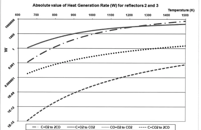
Table 2-1 lists some of the reaction constants for the reactions involved in the air ingress accident. Figure 2-3 and Figure 2-4 show the absolute value of the heat generated by reactions in

(23)

absolute value on a log scale, given a sample reflector surface area and air volume. The reflector used was the same as used on the 2"d and 3rd levels of the NACOK experiments, and the values

used for the reactions are the same as shown in Table 2-1 and discussed in more detail in Section 9.1 for the use in the nodal code. These figures show how dramatically more important the carbon oxidation reaction is as compared to the other reactions, and why the water reaction can be safely neglected for our analysis purposes.

TABLE 2-1: REACTIONS AND CHEMICAL RATE CONSTANTS AND ENERGIES

Reaction Rate constant (A) Activation energy (E)

O+C 7,943 78,300 C02+C 2,220 30,635 CO+02 1.3*10A8 126,000 6 I'0 NN'

Absolute value of Heat Generation Rate (W) for reflectors 2 and 3 Tmpemtum (K)

700 800 900 1000 1100 1200 1300 1400 1500

00

- - C+02to 2CO -C+02to CCC O2 to CO2 ---- C+CO2to2CO -- C+H20toCO+H2 I FIGURE 2-3: ABSOLUTE VALUE OF HEAT GENERATION BY CHEMICAL REACTION FOR A SAMPLE

REFLECTOR GEOMETRY, INCLUDING THE WATER REACTION

23 400 40 ow 00 do as " '00 00 op 'Woole awwww 'W 60,00 0000 10001, 14000 0000" '00e

(24)

Absolute value of Heat Generation Rate (W) for reflectors 2 and 3

Temperature (K)

600 700 800 900 1000 1100 1200 1300 1400 1500

/NO

- c+02 to 2Co -C-O2to C02 --- CO.02to C02 ---- C+CO2to 2C0

FIGURE 2-4: ABSOLUTE VALUE OF HEAT GENERATION BY CHEMICAL REACTION FOR A SAMPLE REFLECTOR GEOMETRY, NOT INCLUDING THE WATER REACTION

Finally, the kinetics of graphite corrosion follow different regimes depending primarily on

temperature. Three primary regimes have been outlined clearly by Moormann et al (16) (17) and are shown graphically in Figure 2-5.

EA ~ 0 EA(CR) 2 EA(CR) Ii II IT In-pore diffusion controlled regime I Chemical regime Ill --Z aj Surface corrosion, gives low strength loss Corrosion (or density-) profile in the porous solid i Homogeneous Smaterial corrosion, 'resulting in high strength iloss

FIGURE 2-5: GRAPHITE CORROSION REGIMES AND EFFECTS ON REACTION RATES (17)

Mass transfer controlled regime

(25)

The regime at the lowest temperature corresponds to the chemical regime. While the reaction rates are lowest in this regime, the oxygen is able to diffuse through the graphite and corrode,

causing high strength loss. The limiting factor is the chemical reaction kinetics alone. At higher temperatures, the reaction takes place more quickly, corresponding to an activation energy of roughly half that in regime I. The amount of diffusion is limited by the higher rate of reaction, so it is said to be in-pore diffusion limited. In regime III, the reaction has an effective activation energy of zero and the reaction occurs as quickly as the oxygen comes in contact with the graphite. Thus, regime III is mass transfer controlled.

2.6. COMPLICATING FACTORS

Common assumptions such as neglecting heat transfer by radiation, assuming ideal gases, bulk temperatures, assuming constant values such as reaction parameters and material properties or neglecting graphite corrosion regimes may strongly affect accurate modeling of the air ingress experiment. In addition, attention must be paid to the graphite corrosion regime and the effect of burnoff on reaction rates. In the case of the FLUENT modeling, the effects of water vapor, radiation, and burnoff have been neglected. However, as described in Section 5, the FLUENT models' results matched closely to the data with these assumptions. The 1-D MATLAB code includes simple accommodations for effects of water vapor on air properties, including: density and specific heat, as well as increase in surface area due to burnoff, and radiative heat transfer, described in section 0.

3. OVERVIEW OF AIR INGRESS EXPERIMENTS

3.1. JAERI

EXPERIMENTS OF EARLY 1990'S AND KUHLMANN NACOK

EXPERIMENTS OF 1999

Several key experiments in recent decades have impacted understanding of the air ingress accident for high temperature gas reactors. Among these are the experiments done by Takeda and Hishida at JAERI (13), and those performed at the NACOK (Naturzug im Core mit

(26)

Korrosion) facility in Germany. MIT began work on CFD modeling of air ingress experiments with the work by Tieliang Zhai and Andrew Kadak characterizing the JAERI experiments of the early 1990s and the NACOK experiments by Kuhlmann in 1999 (16). The JAERI experiments were small scale U-tube experiments which included an experiment examining diffusion and onset of natural convection using two components of nitrogen and helium, and then assessed multicomponent effects of air ingress including diffusion, natural circulation, and chemical reactions as a result of adding a graphite column portion to the first experimental setup (17)(13). Figure 3-1 and Figure 3-2 show the JAERI experimental setups. These experiments were focused on a prismatic geometry, characterized by flow through fuel channels, while the

NACOK experiments were oriented toward the pebble bed reactors setup, which is characterized by flow through fuel pebbles. However, both utilized double-guillotine break assumptions and approximations of upside down U geometry with experimental "hot-" and "cold-leg" flow paths representing the hot reactor interior and the outlet, respectively. Kuhlmann's work similarly addressed air ingress through experiments on the effect of helium on air ingress, the onset of natural convection and the rates of mass flow in a heated column, and the impact of different amounts of helium on mass flow (16). Kuhlmann then performed large scale experiments at NACOK with an experimental setup closer to an actual possible air ingress event as shown in Figure 3-3. The first of the two main experiments performed involved varying temperatures of the hot leg and cold leg and assessing the effects of temperature and geometry on mass flow through ceramic pebbles. Kuhlmann finally applied these results to a second experiment incorporating chemical reactions in a graphite pebble bed.

(27)

Cooler Heaterin 0C-2 -e sampling H o -int Water Wa te-*ufl GTsnk Go

ae-te--8

ga-Conaer 1000 3i M

(28)

1~Gas

Graophite

SOMPINPipe

'Point P

ooler To

(29)

E

.~ ~ ~ ~ . ... .

FIGURE 3-3: NACOK EXPERIMENTAL SETUP

Zhai (7) utilized three 3D FLUENT models to benchmark the JAERI He-N diffusion test, the JAERI multi-component test, and the NACOK ceramic pebble test. The first two were run as

(30)

transient simulations, with the second as a multicomponent model with chemical reactions in the graphite tube portion. The NACOK model was run as a steady state simulation with porous media approximations for the large ceramic pebble area. These models proved to have good agreement to the experimental data as measured by certain parameters such as time for diffusion of nitrogen in the JAERI tests and ceramic pebble bed temperature versus mass flow rate in the NACOK test. FLUENT has been proven to be extremely accurate especially for use of two

component diffusion and for flow and heat transfer scenarios which can be assumed to show steady state behavior. In addition, the FLUENT porous media approximation shows excellent agreement when applied appropriately, e.g. where there are not significant time-dependent effects and disparities in temperature of the fluid and solid in question.

3.2. NACOK EXPERIMENTS OF 2004

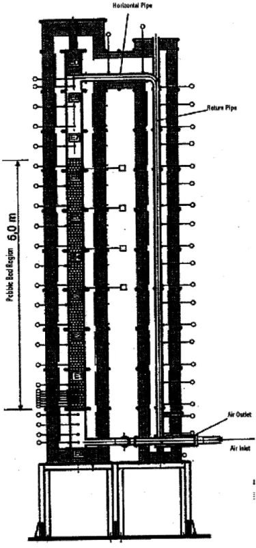
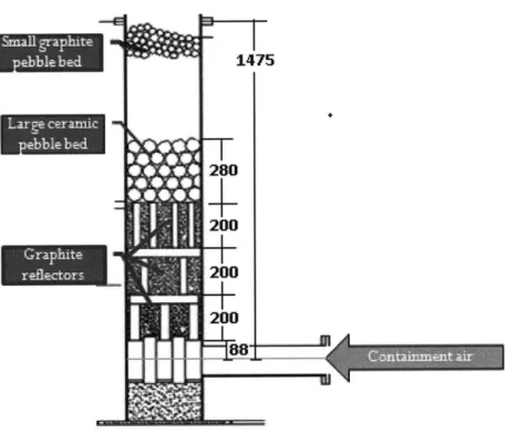
Based on the previous experiments, additional experiments at NACOK were performed in 2004 to gain better understanding of the air ingress processes in pebble bed reactors by utilizing more realistic pebble bed geometries, including multiple levels of graphite reflectors with different channel dimensions and multiple layers of pebbles. Experiments were performed with a simple open chimney and including a return cold leg.

(31)

FIGURE 3-4: NACOK OPEN AND RETURN CHIMNEY HOT LEG SCHEMATIC (DIMENSIONS IN MM)

Figure 3-4 shows a simplified schematic of the open and return chimney set up, which were similar. In the actual set up, the chimney extends upwards past the topmost pebble bed at

1.2m by about 5m. The return leg drawing is far more complex as the chimney not only extends many meters above the pebble bed but also connects horizontally to the equally tall return leg. Figure 3-6 shows a cutout of the drawing for the NACOK return leg experiment.

IND. Lar :e C-9-ramil-I Pebble bed 280 200 200 200 log

(32)

-

--L - - - - --- - - - - - - -

-FIGURE 3-5: NACOK RETURN CHIMNEY SCHEMATIC

For both the open chimney and hot and cold leg experiments, the interior was flushed with hot nitrogen and the walls were electrically heated to a set temperature through the experiment. Air at atmospheric pressure and ambient temperature then flowed through the experimental setup and then reacted with the graphite to heat up the air and graphite. Species and temperature data were taken at certain points in the experiment apparatus over time. The open chimney experiment was run for approximately 8 hours. The return chimney was run for approximately 20 hours,

however after about 4 hours, the reactions and heat produced became out of control and the initial set wall temperatures had to be lowered. Both the open and the return chimney had the same plan for gas sensors, shown in Figure 3-7.

(33)

FIGURE 3-7: GAS SENSOR LOCATIONS IN OPEN AND RETURN CHIMNEY EXPERIMENTS

3.2.1. OPEN CHIMNEY EXPERIMENT

For the open chimney experiment, as described above, the walls were electrically heated to 650C and the chamber was flushed with hot nitrogen. Then the valve was opened, and atmospheric air began to flow through the chimney reflectors and pebbles. Temperature sensors, denoted with the prefix "R," were used for the outer walls to monitor the temperature to be sure the heaters maintained the minimum 650C through the experiment. The thermocouple locations are given in Figure 3-8, which shows both the regulatory temperature sensors and regular thermocouples.

(34)

R1 .2 O8.3 R1.1 T9.3 T 9.2 R3.3 ~3 3 $ T1 3 T1.2

FIGURE 3-8: OPEN CHIMNEY THERMOCOUPLE LOCATIONS

The lowest interior portions are composed of three layers of reflector blocks, supported by four graphite columns. These reflectors are made of ASR-lRS graphite, which has similar properties to IG- 110 graphite used in Japan (18). The first layer of graphite blocks is composed of two blocks, shown in Figure 3-9, each with six cross-drilled channels of 40mm diameter each. The second and third layers each have two blocks, shown in Figure 3-10. The third layer blocks

(35)

are placed with an orientation 90 degrees rotated about the vertical axis relative to the blocks of the second layer. Each block has 48 channels of 16mm diameter each.

FIGURE 3-9: ONE OF TWO FIRST LAYER GRAPHITE BLOCKS

FIGURE 3-10: ONE OF FOUR SECOND AND THIRD LAYER GRAPHITE BLOCKS

Above the reflectors are two pebble regions. The lowest is directly above the third layer of reflectors, and the highest is separated from the first by an empty space. Both pebbles are made of A3-3 graphite (18). The lower pebble bed is made of larger diameter pebbles at 60mm, and the higher pebble bed is made of smaller diameter pebbles at 10mm diameter.

(36)

This experiment is analogous to the open chimney experiment, except that instead of venting the air directly above the pebble bed, the vent at the top is closed and the air passes through the connecting pipe to the cold leg. The connecting pipe at the top of the cold leg was

held to a cooler temperature of between 175C and 200C (18).

In the experimental procedure, the heating elements heat the hot leg to a minimum 850C and instead of nitrogen, the chamber is filled with helium. The air flow was then initiated with an equalized pressure to atmospheric. The flow rate was at a lower constant value than the open chimney as shown in Figure 4-11 versus Figure 4-13 for the open chimney.

(37)

4. THE

2004 NACOK

EXPERIMENTS- REVIEW

OF

DATA

RECEIVED

4.1.THE

OPEN CHIMNEY DATA RECEIVED

The data received for the open chimney experiment included gas species data for helium, oxygen, carbon monoxide and carbon dioxide with time at 9 different vertical locations. The 650 degree C open chimney experiment was run for approximately 8 hours, between 13:09 and 21:09 on 3/10/2004. However, the available data was apparently not taken consistently over this time period. The times of data available at a location may be only for a few hours, while the data on another location may be available in spotty intervals through the full duration of the experiment. Moreover, the data points taken for one species at a location may not start at a similar time or last for a similar duration as the data points taken for another species at the same location. Figure 3-7 illustrates the 6 lower gas sensor locations for the open chimney experiment with respect to the geometry. Figure 4-1, Figure 4-2, and Figure 4-3 show data for the species volume fractions for the 7 most useful gas detector locations. In an ideal gas, the volume fraction is equivalent to a molar fraction and is given by the following:

number of moles of species i

Volume fraction = molar fraction =

total number of moles of all species

(38)

C02 in Open Chimney vs Time (log scale)

-Cl-I, Om, first open chamber

.4-G2,0.268 m, between ist and 2nd ref

-- 63, 0.468 n, between2nd and 3rd ref

--- G4,0.7 m, just above 3rd ref

-'- G.5, 0.760m,just above 1stpeb -+- 6, 1.2 m, upper chimney

--- G7, 6.375 m, topchimney

3/10/200414:24 3/10/2004 16:46 3/10/2004 19:12 3/10/200421:36

FIGURE 4-1: CO2 VOLUME FRACTION IN OPEN CHIMNEY EXPERIMENT

0.1 +

(39)

CO in Open Chimney vs Time (log scale)

1

0.1

0.01

0.001

-- G1,0 in, first open chamber

-4.-62, 0.268 m, between 1st and 2nd ref

- G3,0.468 m, between 2nd and 3rd ref -4K- G4,0.7 m, just above 3rd ref

-- 65,0.760m, just above 1st peb

-- GS, 1.2 m, upper chmney -4-67,6.975 m, topchimney

3/10/200414:24 3/101200416:48 3/10/200419:12 3/10/2004 21:36

FIGURE 4-2: CO VOLUME FRACTION IN OPEN CHIMNEY EXPERIMENT

0.0001 t

(40)

02 in Open Chimney vs Time (log scale)

10--g-G1, O m, first open chamber

>( -- G2, 0.268 m, between ist and 2nd ref

XG3, 0.468 m, between 2nd and 3rd ref

-u-G4, 0.7 m,just above 3rd ref

-- GS, 0.760m, just above 1st peb ---- G6, 1.2 m, upper cmney -- 67, 6.975 m, top chimrney

0.1

0.01-3/10/200412-00 3/10/200414:24 3/10/200416:48 3/10/200419'12 3/10/200421:36

FIGURE 4-3: 02 VOLUME FRACTION IN OPEN CHIMNEY EXPERIMENT

In Figure 4-1 and Figure 4-3, C02 clearly increases while 02 clearly decreases,

respectively, for the duration of the experiment in all locations. This is evidence of the graphite oxidation taking place. The amount of carbon monoxide, shown in Figure 4-2, is less clearly demonstrative of graphite oxidation because the relative amount of carbon monoxide produced in the graphite oxidation reaction is much smaller than for carbon dioxide for the temperatures experienced in the experiment. Moreover, the Boudouard reaction favors consumption of CO and C02 production under about 850C, while above this temperature, the reaction produces CO. Only above about 1OOOC does the much more significant graphite oxidation reaction favor the production of carbon monoxide over carbon dioxide (as shown in Figure 2-4), which is

significantly higher than the maximum temperature reached in this experiment.

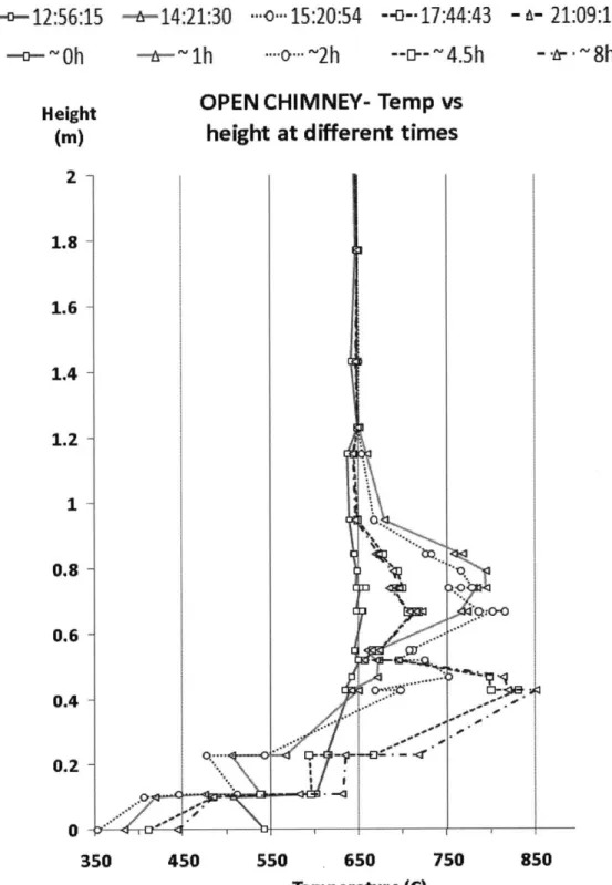
For the open chimney, the temperatures with time were never acquired, and were apparently lost due to an error in the experiment computers. Likewise, mass flow and density data were lost for

(41)

the open chimney experiment. However, an operator's log taken during the experiment was provided, which includes the German operator's abbreviated notes and occasional screen captures of the computer's readings at random points in the experiment. Thus replicating these experiments using computer simulations based on the available data is difficult. Ultimately, temperatures from these log screen captures were used to compare temperatures. The following chart shows the data from the control temperature sensors.

Temperature (C) 750 -725 -700 -675 -650 625 --0:00

Wall Control Temperatures (C) vs. Time

- -0.793 m,R11 - 0.753m R3_3 -- 1.859 m, R1_3 ... 7.417m R3_1

1:00 2:00 3:00 4:00 5:00 6:00 7:00 8:00

Time Elapsed in Experiment(H:MM)

FIGURE 4-4: OPEN CHIMNEY WALL CONTROL TEMPERATURE SENSORS

As can be seen in Figure 4-4, the lower sensors around 0.75-0.80 m. heights, Rl_1 and R3_3, experienced enough heat to increase the temperature of the walls significantly above the 650C minimum set temperature. Figure 3-8 shows the locations of the temperature sensors in the open chimney experiment with respect to geometry.

(42)

---

15:20:54

----

o--

~2h

--o--17:44:43

- -A- - 8h

OPEN CHIMNEY- Temp vs

height at different times

450 550 . 650

Temperature (C)

750 850

FIGURE 4-5: TEMPERATURE VALUES FOR OPEN CHIMNEY COPIED FROM OPERATOR LOG SCREEN CAPTURES

--

14:21:30

-- ~- 1h Height (m) 2 1.8 1.6 1.4 1.2 1 0.8 0.6 0.4 0.2 350

- a- 21:09:18

-<o-12:56:15

(43)

4.2. THE RETURN CHIMNEY DATA RECEIVED

For the return chimney experiment, unlike the open chimney, temperature data with time was not lost and was provided. However, the only species data provided was for oxygen and at two locations, just below the topmost graphitic pebble bed, G6, and measuring the inlet species. The return chimney experiment was conducted over approximately 25 hours between 06:47 on 07/27/2004 and 07:37 on 07/28/2004. Volumetric flow was given throughout the experiment and was shown to be practically constant for 20 of the 25 hours. Figure 4-6, Figure 4-7, and Figure 4-8 show the mass flow rate over the full experiment, the first 5 hours, and compared with the set temperature changes, respectively.

Accumulated Flow ( m3at STP)

s 10 is 20

Time (hours)

(44)

Accumulated Flow ( m3at STP)

0 1 2 3 4 5 6

Time (hours)

FIGURE 4-7: TOTAL ACCUMULATED AIRFLOW IN RETURN CHIMNEY EXPERIMENT OVER FIRST FEW HOURS

Air Flow Volume (m^3)

(45)

Air flow volume (mA3) -Accumulated Flow (m m at STP) - Set Temperature (C) of hot leg Time (hours)

FIGURE 4-8: SET HOT LEG TEMPERATURE COMPARED WITH VOLUMETRIC FLOW IN RETURN CHIMNEY OVER TIME

Figure 4-8 shows that while the air ingress flow rate is relatively constant, the control temperatures for the return chimney experiment varied significantly through the experiment. The overall effect of these changes of the hot leg temperature on the rest of the temperatures in the experiment is shown in Figure 4-9.

600 Temperature 500 (C) 400 300 200 100 0

(46)

Return Chimney Temperatures with time for selected heights Temp (C) 900 -875 850 825 800 775 -750 725 -700 -0 5 10 15 20 Time (h)

FIGURE 4-9: RETURN CHIMNEY TEMPERATURES AT SEVERAL HEIGHTS OVER DURATION OF EXPERIMENT T 2.4,,0.437 m - T 3.2,,0.479 m - - T4.1,,.727 m -T5.2,,0.847 m =-T5.3,,0.972 m --- T 5.4,,1.017 m - T 6.1,,1.476 m

(47)

Return Chimney

Height Temp v height,

(m) differenttimes 1.6 1.4 R G3.3,7/2120:31 1- 31,7/2718:31: 7 / -- 7/27/204 11211 1 -- 7/27/2004 1031 7/27/2004 1331 0.8 -w-- 7/27/2004 14:31 0.---7/27/2004 15,31 0.6 - 7/27/2004 16:31 7/27/2004 1731 0.4 7/27/2004 1831 REG 1.3,712712:31 EG 3,/27U:31 -REG1.3, 7/27 10031 0.2 -- ,2 :REG 3.3, 7/27 10:31 * 1E .3, 7/27 Ae-* REG 1-3, 7/27 18231 0 * REG 3.3, 7/27 500 600 700 Temp. 800 900 1831 (Q

FIGURE 4-10: RETURN CHIMNEY TEMPERATURE (CELSIUS) VS. HEIGHT FOR SELECTED TIMES

(48)

Return Chimney 02 Volume Fraction vs. Time 0.4 0.35 0.3 0.25 0.2

02 LEVEL JUST BELOW

0.15 GRAPHITE COATED PEBBLES 0.1 -- --. . -. 0.05 ...-.- . -- . 0 -0 5 10 15 20 25 Time (h)

FIGURE 4-11: RETURN CHIMNEY 02 VOLUME FRACTION VS. TIME

Figure 4-11 shows that by two hours into the return chimney experiment, there is no appreciable oxygen reaching the topmost pebble bed, at a height of approximately 1.2 meters. This shows that at the very low flow rates for the first few hours, as shown in Figure 4-7, and at these temperatures, the oxidation rates may be low enough that oxygen can travel through a large-scale graphite core without being reacted. However, it may be primarily due to

experimental error, considering there is a significant amount of oxygen at such a height in the reactor at time zero, and the level drops rapidly in the first hour at a low flow rate.

4.3. SUMMARY ON DATA AND INFORMATION CLARITY

The most significant hindrance to the project has been a lack of consistent and complete data from NACOK. Critical portions of data, reports and operator's logs only were also only available in abbreviated German.

(49)

One point of misunderstanding that was finally clarified was that the mass flow rates for both tests seem to have been held constant as opposed to allowed to naturally circulate. The only data we received from the 2 tests regarding mass flow was excel data for total volumetric flow

(mA3) in the return chimney test, apparently taken less frequently than once a minute, and stated

as taken at STP. By taking the change in total volumetric flow in certain time intervals, the volumetric flow per unit time was calculated. Using the density of air at STP (g/mA3), the approximate mass flow per unit time was found.

Mass Flow (g/s) over 15 and 30 min intervals -Return Chimney

X x 4 X + ... ~ X X X X X -- 15 min interval -'30 min interval 0.600 -0.400 - - - - - - - - - - - -.-.-.- - - -. 0.200 0.000 , 0:00 2:24 4:48 7:12 9:36 12:00 14:24 16:48 19:12 21:36

FIGURE 4-12: RETURN CHIMNEY MASS FLOW RATE VS. TIME

For the open chimney experiment, we did not receive any data on mass flow rate. However, an operator's log was provided, which was a document containing hand-written notes from the German operator along with screen captures at a few time points over the course of the experiment. The operator's log provided several points where the "Control" Mass Flow was written down or taken in screen captures:

1.800 1.600 1.400 1.200 1.000 0.800 ... ... ... ..... ... ... ... ... ..... ... ... ...

(50)

"Control" Mass Flow (g/s)- Open Chimney 1 --- - - -... 0.5 0 0:00 1:12 2:24 3:36 ...4 .... 4:48 6:00 7:12 8:24 Time After Beginning of Test (H H:MM)

FIGURE 4-13: OPEN CHIMNEY MASS FLOW RATE VS. TIME

It is also stated in the Operator Log "Konstante... 3.31 g/s" and a single screen capture shows that there is a Control Rate of 2.65-2.68 g/s with a "Regleabweichung" or "Deviation from Control" of about 0.9 g/s. Velocity in a section of the test stand with constant

cross-sectional area is calculated by dividing the volumetric flow rate (m^3/time) by the

cross-sectional area (mA2) to gain velocity (m/time). Because the mass flow rate is constant, the

(51)

Height (m)

1 - - - - -.-.-- -.-.-.-.-.

-empty area before 2nd pebble bed

*first pebble bed .

-6 -- ----0.6 reflector 2 and 3 0.4 reflector 1 0.2.

-

----...

.

....--.-empty room 0 0.02 0.04 0.06 0.08 0.1 0.12 0.14 0.16 Velocity (m/s)

FIGURE 4-14: AIR FLOW VELOCITY IN DIFFERENT CROSS-SECTIONS

Figure 4-14 illustrates the differing velocities found in the experiment given a constant mass flow rate, pressure, and density. The vertical lines do not denote exact locations of the velocities, but rather indicate the relative steps in velocities based on geometries, while the locations of the points do indicate the velocity of air based on geometry at that exact location.

The importance of velocity in the oxidation of graphite is that it supplies more oxygen for oxidation. The Kuhlman reports from NACOK (2) include an equation for oxidation similar to that used by Takeda, with a compensation for velocity. This equation is given in Equation 9-7 and discussed in Section 9.1. However, the contribution of this compensation is quite small. Moreover, the variance from the slow bulk rate of approximately 0.02 m/s to a maximum bulk rate in reflector 1 of 0.14 m/s are both still very low velocities, as should be characteristic of natural convection accidents. These bulk rates are not as important as the surface characteristics and small turbulences at relatively rough surfaces, and the increasing force of viscosity as temperatures heat up post-LOCA.

(52)

5. FLUENT AND

THE

MIT CFD MODELS

FLUENT is an advanced computational fluid dynamics (CFD) software, capable of modeling an array of fluid flow, heat transfer, chemical reactions, diffusion, turbulence, combustion, and other phenomenon. The software can be used to create 2- or 3-dimensional models, explicitly modeled geometry or porous media, and steady state or transient

computations. FLUENT version 6.0 was used both in the prior MIT models and the current work. The array of customizable computational selections and inputs are numerous, however, the most important options are explained here. The grid or mesh is the first step to developing a model. The preprocessing software GAMBIT is provided with FLUENT for building the mesh.

In GAMBIT, the mesh can be created automatically or fine tuned manually. The primary element options are triangular or quadrilateral (3). Triangular meshes generally result in better interpolation across an element, while quadrilateral or tetrahedral can reduce the number of elements required and result in similar or better accuracy if used such that the quadrilateral elements align to the direction of flow, in cases of low turbulence. A key step in generating the mesh is creating zones which will be used in FLUENT to define solid, fluid, and porous areas of the model, along with areas with different material and boundary conditions.

The primary options in FLUENT include the Model Settings, Material Settings, Operating Conditions, Boundary Conditions, and Solver Controls.

5.1. MODEL SETTINGS

The Solver options under the Models setting establishes the critical settings for the way the model case file is calculated. It includes the options of Pressure or Density Based and whether the Superficial or Physical Velocity is used in the Porous Zones. The pressure based solver is generally recommended for low-velocity, incompressible flows, while the density based

solver was developed for high-velocity, compressible flows. Moreover, the pressure based solver is the only choice allowing for the physical velocity formulation for the porous zones. The superficial velocity assumes flow as unobstructed, or the same as outside the porous zone, and does not incorporate the increase in flow velocity due to the smaller volume or pore size.

(53)

Therefore, it is important that the pressure-based solver and the physical velocity options were selected by the previous MIT CFD models and the current work.

The viscosity model can be an important factor in modeling flow; however, previous studies by Brudieu (18) showed that different viscosity settings made little impact in the outcome of a case run. The options available through the viscosity model include: inviscid, laminar, k-epsilon, k-omega, and others. The air flow has a low Reynolds number and could be considered in the laminar flow regime, and this setting was used for the past and present model work at MIT.

The species model is a complex set of options including basics on species and their properties, from thermal to mechanical and transport. The FLUENT database includes libraries of common species properties which can be uploaded. In addition, one is able to select for different methods to input these properties, such as allowing for temperature dependence as

opposed to constant properties. Sub-menus allow for selections regarding the chemical reactions between the species and all of the rates options and inputs necessary to define the reactions and

calculations.

The Operating Conditions menu offers inputs for operating pressure and gravity. It also includes an operating temperature for the Boussinesq calculations. The Boundary Conditions menu is more detailed, with sub-menus with important setting options. Boundary conditions must be set for each zone and wall, inlet and outlet. For fluid zones, the submenus include settings for motion terms, porous media, reactions, and source terms. For solid zones and walls, the submenus include momentum, thermal, radiation, and species, among others. The settings for the inlets and outlets are varied and depend on the outside pressure, pressure drops, defined or free mass flows, etc.

Solver Controls include options for controlling convergence and affecting the numerical methods used by the FLUENT solvers. These options include the pressure-velocity coupling method, and the discretization options, but perhaps the most important setting is that of the under-relaxation factors for the energy, momentum, and species, etc. In the complicated and

(54)

difficult convergence of low-velocity, buoyancy dominated flows, decreasing the under-relaxation factors is a necessary compromise of stiffness and speed for slow convergence.

Setting solution limits also helps guide the solution by reducing the range of variables considered in calculations, for instance, temperature and pressure upper and lower limits. Last, the

initialization of a case can critically determine convergence or divergence of a solution, by setting the zones (including "all zones") to begin computation and by setting reasonable initial values such as temperature, velocities, and species concentrations for those zones.

5.2. THE MIT FLUENT MODELS

FLUENT models of the NACOK experiments were made by M. Brudieu (18) using the Fluent modeling techniques of Zhai (7). Brudieu used 3D models which were first made "blind" (results unknown) in order to assess the ability of the modeling approximations and once some data was received, were modified to more accurately benchmark the tests. Brudieu's final model utilized explicit geometrical modeling only for the lowest reflector, then used separate porous media zones for the next two higher reflectors, and the two pebble zones. Brudieu's Fluent modeling showed good results for both the blind and updated models for temperature distributions but some non-physical temperature drops were found which were further examined in this thesis.

The characteristics of the Brudieu models, especially the final "modified" model of the open chimney are described below. Figure 5-1 shows the mesh of the final open chimney model, and Table 5-1 gives a few important chemical reaction inputs and pressures for all the FLUENT models.

(55)

FIGURE 5-1: MODIFIED FLUENT OPEN CHIMNEY MODEL MESH, LOWER SECTIONS

TABLE 5-1: KEY FLUENT CHEMICAL INPUTS AND PRESSURES FOR BRUDIEU MODELS

Variable/Model Blind Modified Blind Modified

model model model for model for

for open for open return return

chimney chimney duct duct

k Graphite Corrosion 3.6 * 1012 loll 5 * 101 102

EA Graphite corrosion 2.09 * 10* 2.09 * 10* 2.09 * 10* 2.09 * 10*

x/y Stoichiometry 0.86 1.86 1.5 1.5

k Boudonard reaction N.A. N.A. 1000 200

EA Boudouard reaction N.A. N.A. 2.6 * 10 2.6 * 108

Pressure outlet pressure gauge -27.4 Pa -27.4 Pa 0 Pa 0 Pa

k CO oxidation 2.8 * 1012 2.8 * 1012 2.8 * 1012 2.8 * 1012 EA CO oxidation 1.7* 108 1.7* 108 1.7* 108 1.7*108

Analyzing FLUENT CFD models and data to develop fundamental codes to assess the effects of graphite oxidation in an HTGR air ingress accident