Propagation of epistemic uncertainties using dempster-shafer theory in bepu evaluation

HAL Id: hal-02415473

https://hal.archives-ouvertes.fr/hal-02415473

Submitted on 17 Dec 2019

HAL is a multi-disciplinary open access archive for the deposit and dissemination of sci-entific research documents, whether they are pub-lished or not. The documents may come from teaching and research institutions in France or abroad, or from public or private research centers.

L’archive ouverte pluridisciplinaire HAL, est destinée au dépôt et à la diffusion de documents scientifiques de niveau recherche, publiés ou non, émanant des établissements d’enseignement et de recherche français ou étrangers, des laboratoires publics ou privés.

dempster-shafer theory in bepu evaluation

M. Marques, H. Ynuhui, A. Marrel

To cite this version:

M. Marques, H. Ynuhui, A. Marrel. Propagation of epistemic uncertainties using dempster-shafer theory in bepu evaluation. ANS Best Estimate Plus Uncertainty International Conference (BEPU 2018), May 2018, Lucca, Italy. �hal-02415473�

PROPAGATION OF EPISTEMIC UNCERTAINTIES USING DEMPSTER-SHAFER THEORY IN BEPU EVALUATION

M. Marquès, Y. Hou and A. Marrel

CEA, DEN, Centre de Cadarache, F-13108 Saint-Paul-Lez-Durance, France

michel.marques@cea.fr, yunhui.hou@insa-cvl.fr, amandine.marrel@cea.fr

ABSTRACT

BEPU evaluation is generally based on computer simulators such as thermal-hydraulic system codes with expansive computational cost. Furthermore, two types of uncertainties are present in the BEPU evaluation: the aleatory uncertainty which describes the natural variability of random events and the epistemic uncertainty due to lack of knowledge. The former is usually modelled by probability theory where some conditions on data quantity and quality must be satisfied for probability density functions (pdfs) fitting. However, while the epistemic uncertainty is taken into account, with less and imprecise available data (i.e. parameters of physical model and correlations present in the computer simulator), the use of probabilistic methods on uncertainty modelling and propagation cannot be always justified.

The Dempster-Shafer Theory (DST) of evidence provides an adapted framework for representing the parameters with epistemic uncertainty, when it is not possible to build a coherent probabilistic model from the available knowledge. In this theory, instead of pdfs, the parameters are modeled by focal sets with associated degrees of belief. Input uncertainty modeled by DST can be propagated within a BEPU evaluation by mapping input focal sets to the output space. The main problem is how to control the computation cost because the mapped results are obtained by finding the optimal values of the output in each input focal set. In this paper, we propose a new scheme to propagate epistemic uncertainties modelled by DST through a time-consuming computer simulator. Besides classical Monte Carlo method using Cartesian product input mass construction method, we propose a novel procedure using vacuous dimension extension and mass combination rules (e.g. Dempster's combination rule for independent input variables ) after mapping the input focal sets into the output space. This method significantly reduces the number of input focal sets. The obtained output function has less focal sets, but larger range. Thus, a complete coverage of the output focal set space can be provided. Epistemic uncertainty is estimated globally in a conservative point of view. As a result of a trade-off between calculation cost, estimation accuracy and the quantity of details on epistemic uncertainty presented, our proposal enables propagation of epistemic uncertainties modeled by DST with a very limited computation budget making possible its practical use within a BEPU evaluation.

1. INTRODUCTION

The treatment of uncertainties in the analysis of complex system is essential for determining possible ranges on responses of interest such as safety margins or probabilities of exceeding failure criteria. Uncertainties can be categorized according to the character of their sources as either aleatory uncertainties, which represent the intrinsic randomness of a phenomenon, and are irreducible in nature, or epistemic uncertainties, which are reducible uncertainties resulting from lack of knowledge [1, 2, 3]. For aleatory uncertainties, sufficient data can generally enable the definition of input probability distributions and the use of probabilistic methods. By cons, for epistemic uncertainties, data is generally too sparse to enable precise probabilistic descriptions and consequently the uncertainties are often modelled by variation intervals deduced from expert judgment. In this case, the intervals are assimilated to uniform distributions, which enable a probabilistic treatment of epistemic uncertainties.

However in order to skip the limitations of the probabilistic framework, different methods, that we will name extra-probabilistic approaches, have been proposed to model epistemic uncertainties such as fuzzy sets [4], Dempster-Shafer theory of evidence [5, 6], possibility theory [7], probability box (p-box) [8] and random set theory [9]. When both aleatory and epistemic uncertainties are present in the analysis of a complex system, it is often desirable to maintain distinction between both types of uncertainties. A common approach to quantifying the effects of mixed aleatory and epistemic uncertainties is the so-called Second-Order Probability (SOP) analysis [10]. The idea of SOP is to treat separately the aleatory variables and the epistemic variables and to perform a two-stage Monte Carlo simulation, typically by sampling the epistemic variables on the outer loop, then by sampling the aleatory variables on the inner loop. If the result of the inner loop is an empirical distribution of the response of interest, the SOP process yields a family of distributions. Then relevant statistics, such as mean or percentiles, may be computed based on this ensemble and the intervals obtained on the statistics can be interpreted as possible ranges for the statistics given the epistemic uncertainties. In the SOP analysis, the aleatory variables are treated generally by probabilistic methods and the epistemic variables may be considered either by probabilistic methods or by extra-probabilistic approaches, such as interval analysis [10, 11] or Dempster-Shafer theory [11] depending on the assumptions taken for these epistemic variables.

In this paper, we focus on Dempster-Shafer theory of evidence for epistemic uncertainty modeling. Dempster Shafer theory (DST), also known as the theory of belief functions or evidence theory, has been firstly introduced in [5] and then developed in [6]. Epistemic uncertainties are described by sets to which are associated degrees of belief. The challenge is to propagate the input uncertainties modeled by DST into the output space through either numerical simulators or metamodels (in case of too expensive simulators). A local optimization problem is necessary to find the upper and lower bounds of the output for a given set of inputs. For kriging metamodels, efficient global optimization (EGO) algorithm [12] has been proposed as one of the most effective method to solve the global optimization problem. Metamodel is optimized by adding sequentially new points suggested by the algorithm to its learning sample and then updated. But the same problem of computational cost rises as the new points have to be calculated by the expensive simulators. Consequently, the main issue that we have to deal with using EGO is how to reduce the number of new points demanded to be calculated while propagating DST input uncertainty into the output space. For this, we propose a novel scheme to propagate uncertainties modeled by Dempster-Shafer theory through expensive black-box

simulators. The main idea is first to identify the most influential input epistemic uncertainties using new sensitivity indexes proposed in this paper and then to propagate in a detailed way this important parameters while taking into account the other parameters in a more global way. This paper is organized as follows: Dempster-Shafer theory is introduced in Section 2; propagation of mapping function with DST is presented in section 3 with the two possibilities of dimension extension: Cartesian product and vacuous extension; in Section 4, new sensitivity indexes are proposed to study the impact of epistemic uncertainties on the output; the new scheme to propagate epistemic uncertainties modelled by DST through a time-consuming computer simulator is presented in Section 5; finally a numerical application is given in Section 6 to illustrate the efficiency of the proposed method.

2. DEMPSTER-SHAFER THEORY

The Dempster-Shafer theory of evidence (DST) [5,6] provides a flexible framework to represent and combine uncertainty information. The basic assessment function in DST is called the mass function which assigns a degree of belief (mass) to each subset of the whole definition domain 𝛺 (called a frame of discernment) . By definition, 𝛺 = {ω1, ω2, · · · , ωn} is a mutually exclusive set

of hypotheses for which exactly one hypothesis ωi is true. 𝛺 will contain 2n - 1 non-empty

subsets (including 𝛺 itself) as well as the empty set.

Then, given a variable X defined on 𝛺, its mass function is a mapping function: 𝑚Ω_{: 2}Ω_{→ [0,1]}

such that

𝑚(∅) = 0 𝑎𝑛𝑑 ∑ 𝑚(𝐴)

𝐴⊆𝛺

= 1

Where 2𝛺 _{denotes the set containing all subsets of 𝛺, ∅ and 𝛺. All subsets with positive mass are}

called focal sets. Mass function m(A) measures the belief that X exactly belongs to A but not to any subsets of A. The belief affected to 𝛺 is called the degree of ignorance. A mass function is called vacuous if m(𝛺) = 1, which indicates total ignorance on the studied variable. The belief function (bel) and plausibility function (pl) over 𝛺 are defined respectively as:

𝑏𝑒𝑙(𝐴) = ∑ 𝑚(𝐵) 𝐵⊆𝐴 , ∀ 𝐴 ⊆ 𝛺, 𝑝𝑙(𝐴) = ∑ 𝑚(𝐵), 𝐵∩ 𝐴≠ ∅ ∀ 𝐴 ⊆ 𝛺.

Both functions summarize the information from the mass function and interpret it in different ways: the belief function tells the degree of justified support that X lies in A; the plausibility function gives the degree of maximal potential support of the same situation X in A. Moreover, the interval [bel(A), pl(A)] becomes the lower and upper bounds of belief on X in A. For 𝑋 ∈ ℝ, the two functions can be presented as a function of 𝑥 by fixing the form of input sets. The most used ones take the same interval as the definition of cumulative distribution function 𝐹(𝑥), ] − ∞, 𝑥], 𝑥 ∈ ℝ and are defined as

𝑏𝑒𝑙(𝑥) = 𝑏𝑒𝑙(] − ∞, 𝑥]) 𝑝𝑙(𝑥) = 𝑝𝑙(] − ∞, 𝑥])

so that they can also be seen as the bounds of 𝐹(𝑥):

𝑏𝑒𝑙(𝑥) ≤ 𝐹(𝑥) ≤ 𝑝𝑙(𝑥).

Under the framework of DST (in form of mass functions), it is also possible to combine different information sources describing the same variable according to the source reliability and the relation between sources. Among different rules of combination, Dempster’s rule is the most popular one: let m1 and m2 be two reliable independent distinct mass functions describing the

same variable X on 𝛺; the new mass function obtained by combining information from m1 and m2 using Dempster’s rule of combination is given by:

𝑚₁₂(𝐴) =∑𝐵∩ 𝐶=𝐴_{1 − 𝑘}𝑚1(𝐵)𝑚2(𝐶) ∀ 𝐴, 𝐵, 𝐶 ⊆ Ω

where 𝑘 = ∑𝐵∩ 𝐶=∅𝑚1(𝐵)𝑚2(𝐶) represents the conflict between the two mass functions.

Other rules such as cautious rule and disjunctive rule exist to satisfy different conditions [13].

3. PROPAGATION OF MAPPING FUNCTION WITH DST

3.1 Propagation using Dimension Extension with Cartesian Product

Consider a continuous function 𝑓(𝑥): 𝑅𝑑 → 𝑅 taking 𝑑 independent input variables 𝑥 = (𝑥1, … , 𝑥𝑑). Each input variable 𝑥𝑖 is modeled by a mass function 𝑚𝑥𝑖: 2Ωxi → [0,1] where

𝛺𝑥𝑖 ⊆ 𝑅 denotes the definition field of 𝑥_𝑖 so that the mass function of the input 𝑚𝑥: 2Ωx → [0,1] is given by:

𝑚𝑥_(𝑠𝑥_{) = ∏ 𝑚}𝑥𝑖(𝑠𝑥𝑖)

𝑑

𝑖=1

∀𝑠𝑥𝑖 ⊆ 𝛺𝑥𝑖, 𝑖 = 1, . . , 𝑑

where 𝑠𝑥 is a Cartesian product of subsets on all input dimensions , i.e. 𝑠𝑥 = 𝑠𝑥𝑖× . . .× 𝑠𝑥𝑑 and the definition field of 𝑥, 𝛺𝑥 = 𝛺𝑥𝑖× . . .× 𝛺𝑥𝑑_{. We notice that the focal sets of input mass} function are the Cartesian products of focal sets of mass functions on each input dimension. Then the mass function of the output 𝑦 = 𝑓(𝑥) can be defined as follows

𝑚𝑦_(𝑔(𝑠𝑥_{)) = 𝑚}𝑥_(𝑠𝑥₎

where function 𝑔: 2Ωx

→ 2Ωy

maps a set of input values to its correspondent output space which includes all possible output values given by the input set, i.e.

{𝑦 = 𝑓(𝑥)|∀𝑥 ∈ 𝑠𝑥_{} ⊆ 𝑔(𝑠}𝑥_).

With the continuity of 𝑓, we can easily define the set mapping function 𝑔 as follows: 𝑔(𝑠𝑥_{) = [ 𝑚𝑖𝑛}

𝑥∈ 𝑠𝑥𝑓(𝑥) , 𝑚𝑎𝑥_{𝑥∈ 𝑠}𝑥 𝑓(𝑥)] ∀ s

x _{⊆ Ω}x_. 3.2 Propagation using Dimension Extension with Vacuous Extension

An alternative method is to propagate the mass function of each variable to the output space with vacuous mass functions on the other dimensions and then merge the partial output mass functions with Dempster’s rule of combination (shown in Algorithm 0)

The number of multidimensional input focal sets to be propagated to the output space is the sum of number of focal sets of all unidimensional input variables. Compared to the number obtained by the former method which is equal to the product of the focal set number of all variables, here the number of optimization searches demanded during the propagation is largely reduced. For

example, if there are 4 input variables defined each by 3 focal sets, the number of multidimensional input focal sets to be propagated will be 34 _{= 81 with Cartesian product and} only 4 x 3 =12 with vacuous extension. Vacuous extension avoids the fast calculation cost

increase as more input variables are taken into account, which is very important for expensive optimization operations.

Algorithm 0: initial proposal with vacuous extension

Step 1: construct partial multidimensional input mass function for each input variable 𝑥_𝑖 (𝑖 = 1, … , 𝑑)

𝑚_𝑖𝑥(𝑠_𝑖𝑥_{) = {𝑚}𝑥𝑖(𝑠𝑥𝑖) 𝑖𝑓 𝑠𝑖𝑥= 𝛺𝑥1 × ⋯ 𝑠𝑥𝑖× ⋯ × 𝛺𝑥𝑑

0 𝑜𝑡ℎ𝑒𝑟𝑤𝑖𝑠𝑒

Step 2: construct the partial output mass functions 𝑚_𝑖𝑦 by propagating separately 𝑚_𝑖𝑥 to the output space (𝑖 = 1, … , 𝑑) 𝑚_𝑖𝑦(𝑔(𝑠_𝑖𝑥_{)) = 𝑚} 𝑖𝑦([ 𝑚𝑖𝑛_{𝑥∈ 𝑠} 𝑖 𝑥𝑓(𝑥) , 𝑚𝑎𝑥_{𝑥∈ 𝑠} 𝑖 𝑥𝑓(𝑥)]) = 𝑚𝑖 𝑥_(𝑠 𝑖𝑥) (1)

Step 3: merge all partial output mass functions 𝑚_𝑖𝑦 (𝑖 = 1, … , 𝑑) into one final output function

𝑚𝑦 _{using Dempster’s rule of combination}

𝑚𝑦 _{= 𝑚}

1𝑦⊗ … ⊗ 𝑚𝑑𝑦.

4. SENSITIVITY ANALYSIS WITH EPISTEMIC UNCERTAINTY

In this section, we propose firstly two measures of epistemic uncertainty and then new sensitivity indexes useful within DST using the propagation results introduced in the previous section.

4.1 Existing Sensitivity Indexes

Sensitivity analysis studies the impact of the variation of input variables on the output. In probability theory, variance analysis, where variance is used as a measure of dispersion, is widely applied. The first-order sensitivity index of an input variable 𝑋𝑖, introduced by I.M. Sobol

[14], is defined as follows:

𝑆_𝑖 =𝑉𝑎𝑟(𝐸(𝑌|𝑋𝑖)) 𝑉𝑎𝑟(𝑌)

It measures the effect on output variance of varying 𝑋_𝑖 alone, but averaged over variations in other input parameters; therefore it represents the contribution to the output variance of the main effect of 𝑋_𝑖. So its value is large when the contribution of 𝑋_𝑖 is important.

Similar to variance method, for imprecise probability, a p-box method is proposed in [15] which quantifies the aleatory and epistemic uncertainties by surface between the upper and lower cumulative distribution functions of the output. The p-box sensitivity index is given by:

𝑆_𝑖𝑝 = 𝐴𝑖 𝐴 =

∫ (𝐹_𝛺′ 𝑖(𝑦) − 𝐹𝑖(𝑦)) 𝑑𝑦

∫ (𝐹(𝑦) − 𝐹_𝛺′ (𝑦)) 𝑑𝑦

where 𝐹 and 𝐹 are the upper and lower cumulative distribution functions estimated over the whole variation domains of all input variables and 𝐹𝑖 and 𝐹𝑖 are the ones obtained over the whole

variation domains of variables 𝑋𝑖 with given default values for the other input variables. It

indicates the global importance in terms of uncertainty of 𝑋𝑖 on the output. 4.2 Proposed Measures of Epistemic Uncertainty

We propose to measure the epistemic uncertainty based on the surface constituted by the mass function or by the surface bounded by the belief and plausibility functions on ] − ∞, 𝑥], ∀ 𝑥 ∈ Ω ⊆ ℝ, i.e. 𝐴𝑚𝑎𝑠𝑠 = ∫ ∫ 𝑚([𝑎, 𝑏])(𝑏 − 𝑎)𝑑𝑏𝑑𝑎 𝑏∈Ω 𝑎∈Ω 𝐴𝑏𝑒𝑙𝑝𝑙 = ∫ [ 𝑝𝑙(] − ∞, 𝑥]) − 𝑏𝑒𝑙(] − ∞, 𝑥])] 𝑑𝑥. 𝑥∈Ω

The measure 𝐴𝑚𝑎𝑠𝑠 depends on the range and mass value of the focal sets of the mass function 𝑚. The value of 𝐴𝑚𝑎𝑠𝑠 will increase if the range of any focal set becomes larger for an unchanged mass value. The measure 𝐴𝑏𝑒𝑙𝑝𝑙 has the same property as it just summarizes the information provided by the mass function.

𝐴𝑚𝑎𝑠𝑠and 𝐴𝑏𝑒𝑙𝑝𝑙 measure the epistemic uncertainty in a mass function: smaller (or larger) 𝐴𝑚𝑎𝑠𝑠and 𝐴𝑏𝑒𝑙𝑝𝑙 values signify more (or less) precise information and less (or more) epistemic uncertainty provided by the mass function; the maximum values (𝐴_Ω𝑚𝑎𝑠𝑠 _{= 𝐴}

Ω

𝑏𝑒𝑙𝑝𝑙 _{= max}

𝑥∈Ω 𝑥 −

min

𝑥∈Ω𝑥) come from a vacuous mass function, i.e. 𝑚(Ω) = 1, which corresponds the notion of

total ignorance (maximal degree of epistemic uncertainty); probability cumulative distributions, which can also be seen as mass functions whose focal sets are only singletons ({𝑥}), produce the minimums of both measures (𝐴_𝐹𝑚𝑎𝑠𝑠 _{= 𝐴}

𝐹

𝑏𝑒𝑙𝑝𝑙 _{= 0).} 4.3 New Sensitivity Indexes

The initial idea of our proposed sensitivity indexes is to compare the difference on degree of epistemic uncertainty over the obtained output mass function with and without information provided by the mass function describing a certain input variable. The degree of epistemic uncertainty is measured by 𝐴𝑚𝑎𝑠𝑠 or by 𝐴𝑏𝑒𝑙𝑝𝑙, defined previously.

In order to avoid fixing a default values for the input variable, as in the existing indexes (§4.1), we propose to characterize the effect of variable 𝑋_𝑖 by the partial output function 𝑚_𝑖𝑦 obtained in Step 2 of algorithm 0. Indeed, each focal set of 𝑚_𝑖𝑦 is obtained by searching the optimums of the output over one corresponding focal set for 𝑋_𝑖 and the whole field for the other input variables.

According to (1), the range of the output focal sets shows the impact of variation of 𝑋_𝑖 on the output in term of degree of epistemic uncertainty.

Therefore we define the ratios 𝐴𝑦𝑖 𝑚𝑎𝑠𝑠 𝐴_Ω𝑦𝑚𝑎𝑠𝑠 and 𝐴_𝑦𝑖𝑏𝑒𝑙𝑝𝑙 𝐴_Ω𝑦𝑏𝑒𝑙𝑝𝑙 where 𝐴𝑦𝑖 𝑚𝑎𝑠𝑠_{or 𝐴} 𝑦𝑖 𝑏𝑒𝑙𝑝𝑙

denote respectively the surfaces created by 𝑚_𝑖𝑦 and 𝑏𝑒𝑙_𝑖𝑦/𝑝𝑙_𝑖𝑦, i.e.

𝐴_𝑦𝑚𝑎𝑠𝑠_{𝑖 = ∫ 𝑚} 𝑖𝑦(𝑠)|𝑠|𝑑𝑠 2Ωy = ∑ 𝑚(𝑠 𝑥𝑖)[ max 𝑥∈(×j≠i Ω𝑥𝑗) ×𝑠𝑥𝑖 𝑀(𝑥) − min 𝑥∈(×j≠i Ω𝑥𝑗) ×𝑠𝑥𝑖 𝑀(𝑥)] 𝑠𝑥𝑖⊆Ω𝑥𝑖 𝐴𝑏𝑒𝑙𝑝𝑙_𝑦𝑖 = ∫ 𝑝𝑙_𝑖𝑦(] − ∞, 𝑥] ) − 𝑏𝑒𝑙_𝑖𝑦(] − ∞, 𝑥] )𝑑𝑥 𝑥∈ℝ and 𝐴_Ω𝑚𝑎𝑠𝑠 _{= 𝐴} Ω 𝑏𝑒𝑙𝑝𝑙

is the surface constituted by the mass function of the response obtained by vacuous extension.. They represent the ratios of output epistemic uncertainty given only the mass function of 𝑋𝑖 and with total ignorance on all input variables. They measure the diminution of

epistemic uncertainty on the output while the available information on 𝑋𝑖 is added in DST. As

the measures become larger, the focal sets of 𝑚_𝑖𝑦cover larger range and show less impact on limiting the output value variation. On the contrary, a smaller measure indicates that the focal sets of 𝑚𝑥𝑖 _{plays an important role on reducing the epistemic uncertainty and variation of the} output.

Finally the sensitivity indexes that we propose are defined as follows:

𝑆_{𝑚𝑎𝑠𝑠}𝑦𝑖 _{= 1 −}𝐴𝑦𝑚𝑎𝑠𝑠𝑖 𝐴_Ω𝑚𝑎𝑠𝑠𝑦 , 𝑆_{𝑏𝑒𝑙𝑝𝑙}𝑦𝑖 _{= 1 −}𝐴𝑦𝑖 𝑏𝑒𝑙𝑝𝑙 𝐴𝑏𝑒𝑙𝑝𝑙_Ω𝑦 𝑆_{𝑚𝑎𝑠𝑠}𝑦𝑖

and 𝑆_{𝑏𝑒𝑙𝑝𝑙}𝑦𝑖 can be seen as sensitivity measures of epistemic input uncertainty on output within the framework of DST.

5. MIXED SCHEME PROPOSAL

The ranking of the 𝑆_{𝑚𝑎𝑠𝑠}𝑦𝑖 _{and/or the 𝑆}

𝑏𝑒𝑙𝑝𝑙𝑦𝑖 over all input variables (𝑖 = 1, … , 𝑑), makes possible

the selection of the most influential epistemic variables, that is the ones which reduce significantly the range output focal sets and provide more precise information on the output. We know that dimension extension with Cartesian product gives more input focal sets and details but is more costly; and that the vacuous method needs less calculation resources but provides very conservative result and larger epistemic uncertainty estimate. In order to improve the algorithm (Algorithm 0) initially proposed while keeping the advantage of vacuous extension and adding more precise information, an improved algorithm (Algorithm 1) is proposed using both methods: for input variables with evident impact on output mass function, dimension extension using Cartesian product is used; for other less influential variables, vacuous extension is applied. The selection of influential input variables is determined according to the ranking the 𝑆_{𝑚𝑎𝑠𝑠}𝑦𝑖 and/or the 𝑆_{𝑏𝑒𝑙𝑝𝑙}𝑦𝑖

The cost of this calculation is limited by the number of input variables chosen in Step 3 and the propagation method in Step 4. Since the number of focal sets of the multidimensional mass function obtained in Step 3 by Cartesian dimension extension is equal to the product of numbers of focal sets of all the selected variables, the number of focal sets to be propagated is controlled by limiting the number of selected variables. It is also possible to use Monte-Carlo method instead of complete propagation over all focal sets in Step 4 in order to reduce computation cost.

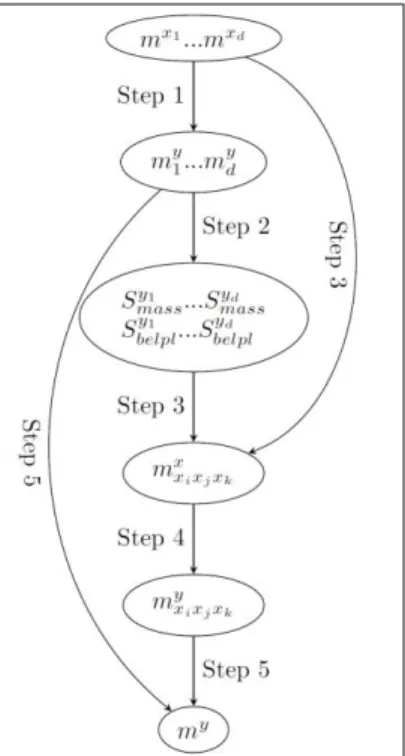
Algorithm 1: Improved algorithm (mixed scheme) (see Figure 1))

Step 1: calculate the partial mass functions of the output 𝑚_𝑖𝑦, (𝑖 = 1, … , 𝑑) with vacuous

dimension extension, i.e.

𝑚_𝑖𝑦(𝑔(𝑠_𝑖𝑥_{)) = {𝑚}𝑥𝑖(𝑠𝑥𝑖) 𝑖𝑓 𝑠𝑖𝑥 = Ω𝑥1× ⋯ 𝑠𝑥𝑖 × ⋯ × Ω𝑥𝑑

0 𝑜𝑡ℎ𝑒𝑟𝑤𝑖𝑠𝑒

Step 2: calculate sensitivity indexes of epistemic uncertainty 𝑆_{𝑚𝑎𝑠𝑠}𝑦𝑖 and 𝑆_{𝑏𝑒𝑙𝑝𝑙}𝑦𝑖 and select the input variables (e.g. 𝑋_𝑗 and 𝑋_𝑘) with greatest 𝑆_{𝑚𝑎𝑠𝑠}𝑦𝑖 _{and/or 𝑆}

𝑏𝑒𝑙𝑝𝑙𝑦𝑖 values

Step 3: merge mass functions of the selected input variables by Cartesian dimension extension,

for example

Step 4: propagate the merged mass function into the output space while the search area of the

non-selected parameters is the whole definition field

Step 5: combine the mass function obtained in Step 4 with the partial output mass functions

obtained in step1 of the non-selected parameters

6. NUMERICAL APPLICATION

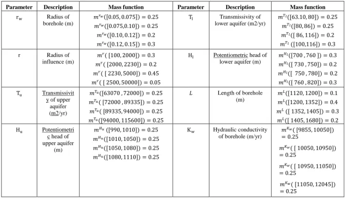
The benchmark we used to illustrate and test our proposed methods is the Borehole function [16] with eight independent input variables. This Borehole function models water flow through a borehole. It is widely used for testing a wide variety of methods in computer experiments thanks to its simplicity and quick evaluation. The output is the water flow rate (in m3/yr) calculated as follows: 𝑓(𝑥) = 2𝜋 𝑇𝑢 (𝐻𝑢− 𝐻𝑙) 𝑙𝑛(𝑟/𝑟_𝑤)(1 + 2𝐿𝑇𝑢 𝑙𝑛 (_𝑟𝑟 𝑢) 𝑟𝑤 2_𝐾 𝑤 +𝑇𝑢 𝑇_𝑙)

Instead of modelling the input variables by probability density functions as is usually done in the classical BEPU evaluation, the input variables are here modelled by mass functions (shown in Table 1). For the purpose of this numerical application, the values associated to the mass functions have been arbitrary chosen but in a real application they may have been obtained by expert elicitation. For example, the mass function of the variable Hu (shown in Figure 2) may

correspond to the judgement of one expert giving the input range of the variable and three quantiles (25%, 50% and 75%) or to the combination of several expert judgements. In all cases, this type of representation by mass function enables to handle, in case of epistemic uncertainty, less precise information than probability density functions.

Parameter Description Mass function Parameter Description Mass function

rw Radius of borehole (m) 𝑚𝑟𝑤([0.05, 0.075]) = 0.25 𝑚𝑟𝑤([0.075,0.10]) = 0.25 𝑚𝑟𝑤_{([0.10, 0.12]) = 0.2} 𝑚𝑟𝑤_{([0.12, 0.15]) = 0.3} Tl Transmissivity of lower aquifer (m2/yr)

𝑚𝑇𝑙_{([63.10, 80]) = 0.25} 𝑚𝑇𝑙([80, 86]) = 0.25 𝑚𝑇𝑙_{([ 86, 116]) = 0.2} 𝑚𝑇𝑙 _{([100,116]) = 0.3} r Radius of influence (m) 𝑚𝑟_{( [100, 2000]) = 0.3} 𝑚𝑟_{( [2000, 2230]) = 0.2} 𝑚𝑟_{( [ 2230, 5000]) = 0.45} 𝑚𝑟_{( [ 2500, 50000]) = 0.05} Hl Potentiometric head of lower aquifer (m) 𝑚𝐻𝑙_{([700 , 760 ]) = 0.3} 𝑚𝐻𝑙_{([ 730 , 750]) = 0.2} 𝑚𝐻𝑙_{([ 750 , 780]) = 0.2} 𝑚𝐻𝑙_{([ 760 , 820]) = 0.3} Tu Transmissivit y of upper aquifer (m2/yr) 𝑚𝑇𝑢_{([63070 , 72000]) = 0.25} 𝑚𝑇𝑢_{( [72000 , 89335]) = 0.25} 𝑚𝑇𝑢_{( [89335, 94000]) = 0.25} 𝑚𝑇𝑢_{([94000, 115600]) = 0.25} 𝐿 Length of borehole (m) 𝑚𝐿_{([1120, 1200]) = 0.1} 𝑚𝐿_{([1200, 1352]) = 0.4} 𝑚𝐿 _{([ 1352, 1405]) = 0.3} 𝑚𝐿_{([ 1405, 1680]) = 0.2} Hu Potentiometri c head of upper aquifer (m) 𝑚𝐻𝑢 _{([990, 1010]) = 0.25} 𝑚𝐻𝑢_{([1010, 1050]) = 0.25} 𝑚𝐻𝑢_{([1050, 1080]) = 0.25} 𝑚𝐻𝑢([1080, 1110]) = 0.25 Kw Hydraulic conductivity of borehole (m/yr) 𝑚𝐾𝑤_{( [9855, 10050])} = 0.25 𝑚𝐾𝑤_{( [ 10050, 10950])} = 0.25 𝑚𝐾𝑤_{( [ 10950, 11050])} = 0.25 𝑚𝐾𝑤_{( [11050, 12045])} = 0.25

Figure 2 – Mass function of variable Hu (Bel = belief function and Pl = plausibility function)

In this example, optimization search for the corresponding output focal sets are conducted by a genetic method provided by R package rgenoud [17].

After executing Step 2, two or three input variables are selected according to their sensitivity measures (Table 2). When three variables are selected, the choices based on one or the other of the two indexes are the same (rw, Hu ,L). When two variables are selected, the choices are

slightly different: (rw, L) according to 𝑆_{𝑚𝑎𝑠𝑠}𝑦𝑖 and (rw, Hu) according to 𝑆_{𝑏𝑒𝑙𝑝𝑙}𝑦𝑖 .

Input variable 𝑨𝒚𝒊 𝒎𝒂𝒔𝒔 _𝑨 𝒚𝒊 𝒃𝒆𝒍𝒑𝒍 𝑺𝒎𝒂𝒔𝒔𝒚𝒊 𝑺𝒃𝒆𝒍𝒑𝒍𝒚𝒊 rw 160.5616 212.9625 0.468 0.2942 r 301.0632 301.2724 0.002 0.002 Tu 301.7553 301.7556 << 0.001 << 0.001 Hu 263.9355 282.8121 0,125 0.063 Tl 301.3379 301.5718 0.001 < 0.001 Hl 274.2439 284.0597 0,091 0.059 L 263.6856 283.5106 0.126 0.060 Kw 277.4571 288.1576 0.081 0.045

Table 2 - Borehole function – Epistemic sensitivity measures On Step 4, the input mass functions 𝑚_𝑟𝑥_{𝑤𝐻𝑢(or 𝑚}

𝑟𝑤L

𝑥 _{) and 𝑚} 𝑟𝑤𝐻𝑢𝐿

𝑥 _{containing the information on}

the selected input variables extended using Cartesian product method with ignorance on the other variables are propagated to the output space. Then we obtain the corresponding output mass functions 𝑚_𝑟𝑦_𝑤𝐻𝑢 (or 𝑚_𝑟𝑦_𝑤𝐿) and 𝑚_𝑟𝑦_{𝑤𝐻𝑢𝐿}. Compared with the output mass functions 𝑚_𝑟𝑦_𝑤⊗ 𝑚_𝐻𝑦_𝑢and 𝑚_𝑟𝑦_𝑤⊗ 𝑚_𝐻

𝑢

𝑦 _{⊗ 𝑚}

𝐿𝑦, intermediate results obtained on Step 3 in Algorithm 0 and

containing exactly the same information, these new intermediate results show smaller value on 𝐴𝑦𝑚𝑎𝑠𝑠 and 𝐴𝑏𝑒𝑙𝑝𝑙𝑦 and indicate less epistemic uncertainty and a more precise description of the

Method Selected input variables 𝑨𝒚𝒎𝒂𝒔𝒔 𝑨𝒚𝒃𝒆𝒍𝒑𝒍 Algorithm 0 (rw, Hu) 149.3 192.3 (rw, L) 147.4 195.1 (rw, Hu ,L) 144.7 185.5 Algorithm 1 (rw, Hu) 132.5 147.4 (rw, L) 133.5 147.6 (rw, Hu ,L) 106.6 110.8

Table 3 - Sensitivity measures of intermediate results

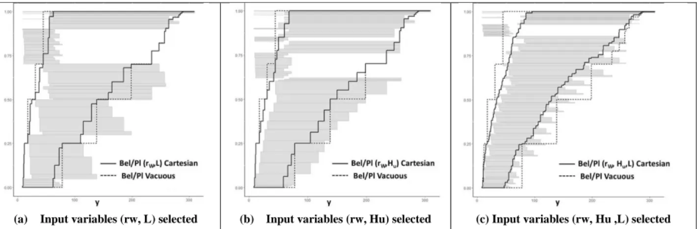
Since the next operation (i.e. merging these intermediate results with the other partial output mass functions using Dempster’s rule of combination) is the same for both intermediate results it is normal to observe similar results in the final results (shown in Figure 3 and Table 4): the final output mass function obtained by Algorithm 1 is less conservative than the one obtained by Algorithm 0 using vacuous extension. The rapid decrease on epistemic uncertainty measures as more input variables enter into Step 2 corresponds well to our initial objectives.

Table 4 gives also the number of output focal sets and so an idea of the calculation costs in each case. The mixed scheme proposed in Algorithm 1 can be seen as an intermediate solution between Algorithm 0 with complete vacuous extension and the method with total Cartesian extension before propagation. Starting with Algorithm 0, as more variables are selected, this improved method tends to the latter one, presenting less epistemic uncertainty and more details but becoming more costly.

As Cartesian product method using complete propagation (or Monte-Carlo simulations) through expensive simulators is generally impossible, this improved method enables a trade-off, within a BEPU evaluation, between the calculation costs and how conservative is the final output mass function.

(a) Input variables (rw, L) selected (b) Input variables (rw, Hu) selected (c) Input variables (rw, Hu ,L) selected

Figure 3 - Borehole function –1) mass functions (rectangles) and Bel/Pl functions (solid lines) of the output obtained by Algorithm 1 with 2 or 3 input variables selected 2) Bel/Pl functions of the

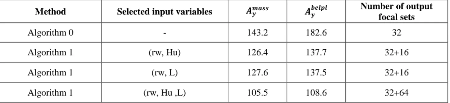
Method Selected input variables 𝑨𝒚𝒎𝒂𝒔𝒔 𝑨𝒚𝒃𝒆𝒍𝒑𝒍 Number of output _{focal sets}

Algorithm 0 - 143.2 182.6 32

Algorithm 1 (rw, Hu) 126.4 137.7 32+16

Algorithm 1 (rw, L) 127.6 137.5 32+16

Algorithm 1 (rw, Hu ,L) 105.5 108.6 32+64

Table 4 - Borehole function - sensible measures of the finally obtained output mass functions using different proposed methods (Algorithm 0 and Algorithm 1)

7. NUCLEAR POWER PLANT APPLICATION

Our method has been applied within the framework of a BEPU analysis of a “Loss Of Coolant Accident” (LOCA) in a pressurized water reactor. The thermal-hydraulic analysis is performed by the CATHARE2 code [18]. In our application, 27 independent CATHARE2 input parameters related to the modeling of physical phenomena (e.g. friction or condensation coefficients) are considered as epistemic uncertainties. The response of interest calculated by CATHARE2 is the maximal peak cladding temperature (PCT), obtained during the LOCA transient. The objective of our analysis is to quantify the epistemic uncertainty of the PCT and to identify among the 27 input parameters the most important contributors to this uncertainty.

The mass functions of the input parameters have been built from the information, obtained by expert judgement, on their ranges of variation and on three quantiles (25%, 50% and 75%). Thus each input parameter is defined by 4 focal sets.

Due to the large cpu-time cost associated to each evaluation by the CATHARE2 code, an improved optimization for the search of the output (i.e. PCT) focal sets has been used. The optimisation scheme used is based on the efficient global optimization (EGO) algorithm [12] where the computer code is surrogated by a kriging metamodel. In order to build this metamodel, CATHARE2 simulations are performed following a design of experiments based on a space-filling LHS. In our approach, the EGO algorithm has been adapted to locally (i.e. at the level of a focal set) improve the accuracy of the metamodel for optimization purpose.

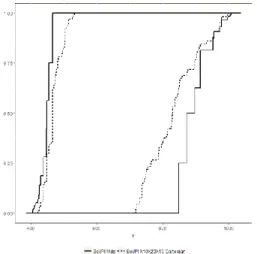
As for the Borehole function (see section 6), we have compared, in Figure 4, the results obtained by vacuous extension and Dempter’s rule (algorithm 0) and by the mixed scheme (algorithm 1). In the mixed scheme, the two or three most important input parameters have been identified thanks to the calculation of the epistemic sensitivity indexes (see section 4.3). For algorithm 0, the number of focal sets to be propagated is equal to 108 (i.e. 27 x 4); for algorithm 1, it is 124 (i.e. 27 x 4 + 42) when two parameters are selected or 172 (i.e. 27 x 4 + 43) when three parameters are selected. In the last case, the corresponding number of CATHARE2 simulations necessary to evaluate the output mass function, is 698.

This application shows the possibility of applying the DST in the case of a large number of input epistemic variables (27 in our case). Algorithm 0 gives a complete but conservative global representation of the simulator response (i.e. the PCT). In the case of using the mixed scheme, the domain delimited by the belief and plausibility functions is substantially reduced, allowing a less conservative representation of the PCT epistemic uncertainty. The interest of this mixed

scheme for propagating epistemic uncertainties with DST is also to adapt the number of selected input variables (in Step 2) to the calculation budget.

Figure 4 – LOCA application – Belief and plausibility functions of the response (PCT) obtained by the mixed scheme with three selected parameters (dashed lines) and by the algorithm 0 (solid

lines)

8. CONCLUSION

In this paper, we have first proposed new sensitivity indexes focusing on epistemic uncertainty useful within the framework of DST. Then we have proposed a new scheme to propagate epistemic uncertainties modelled by DST through a time-consuming computer simulator. Starting from a selection of the most influential input variables based on these new sensitivity indexes, the method consists in using dimension extension by Cartesian product for input variables with evident impact on output mass function and to apply vacuous extension for other less influential variables. Finally, mass combination rules (e.g. Dempster's combination rule for independent input variables) are used after mapping the input focal sets into the output space. Besides classical Monte Carlo method using Cartesian product input mass construction method, this method significantly reduces the number of input focal sets. The obtained output function has less focal sets, but larger range. Thus, a complete coverage of the output focal set space can be provided. Epistemic uncertainty is estimated globally in a conservative point of view. As a result of a trade-off between calculation cost, estimation accuracy and the quantity of details on epistemic uncertainty presented, our proposal enables propagation of epistemic uncertainties modeled by DST with a limited computation budget making possible its practical use within a BEPU evaluation.

9. REFERENCES

[1] A. Der Kiuriegan, “Aleatory or epistemic? Does it matter ?” Special Workshop on Risk

Acceptance and Risk Communication, Stanford University, March 26-27, 2007.

[2] J.C Helton, “Quantification of margins and uncertainties: conceptual and computational basis”. Reliability Engineering and System Safety. 96, 976-1013, 2011.

[3] L.P. Swiler et al, “Epistemic uncertainty in calculation of margins”. 50th AI-AA/ASME,

Structures, Structural Dynamics, and Materials Conference, Palm Springs, USA, 4-7

May 2009.

[4] B. Möller, “Fuzzy randomness ; a contribution to imprecise probability”, ZAMM-Journal

of Applied Mathematics and Mechanics 84 (10-11) (2004) 754-764.

[5] A. P. Dempster, “Upper and lower probabilities induced by a multivalued mapping”, The

annals of mathematical statistics (1967) 325-339.

[6] G. Shafer, “A mathematical theory of evidence”, Vol. 1, Princeton University press, 1976.

[7] D. Dubois, H. Prade, “Possibility theory: an approach to computerized processing of uncertainty”, Springer Science & Business Media, 2012.

[8] S. Ferson, L. R. Ginzburg, “Different methods are needed to propagate ignorance and variability”, Reliability Engineering & System Safety 54 (2-3) (1996) 133{144.

[9] G. Matheron, “Random sets and integral geometry”, Wiley series in probability and

mathematical statistics, Wiley, 1975.

[10] M.S. Eldred et al, “Mixed aleatory-epistemic uncertainty quantification with stochastic expansions and optimization-based interval estimation”, Reliability Engineering and

System Safety 96, 1092–1113, 2011.

[11] M. Marquès, “Propagation of aleatory and epistemic uncertainties in quantification of systems failure probabilities or safety margins”, Safety and Reliability: Methodology and

Applications – Nowakowski et al. (Eds), 2015.

[12] D. R. Jones, M. Schonlau, W. J. Welch, “Efficient global optimization of expensive black-box functions”, Journal of Global optimization 13 (4) (1998) 455-492.

[13] T. Doneux, “Conjunctive and disjunctive combination of belief functions induced by nondistinct bodies of evidence”, Artificial Intelligence 172 (2008) 234–264.

[14] I. M, Sobol. "Sensitivity estimates for nonlinear mathematical models." Mathematical

Modelling and Computational Experiments 1.4 (1993): 407-414.

[15] J. Guo, X. Du, “Sensitivity analysis with mixture of epistemic and aleatory uncertainties”,

AIAA Journal 45:9 (2007), 2337-2349.

[16] M. D. Morris, T. J. Mitchell, D. Ylvisaker, “Bayesian design and analysis of computer experiments: use of derivatives in surface prediction”, Technometrics 35 (3) (1993) 243-255.

[17] W. R. Mebane, J. S. Sekhon, “Genetic optimization using derivatives: The rgenoud Package for R”, Journal of Statistical Software, (2011).

[18] P. Mazgaj, J.L. Vacher, S. Carneval, “Comparison of CATHARE results with the experimental results of cold leg intermediate break LOCA obtained during ROSA-2/LSTF test 7”, EPJ Nuclear Sciences and Technologies, 2 (1), 2016.