HAL Id: cea-01502283
https://hal-cea.archives-ouvertes.fr/cea-01502283
Submitted on 5 Apr 2017
HAL is a multi-disciplinary open access
archive for the deposit and dissemination of
sci-entific research documents, whether they are
pub-lished or not. The documents may come from
teaching and research institutions in France or
abroad, or from public or private research centers.
L’archive ouverte pluridisciplinaire HAL, est
destinée au dépôt et à la diffusion de documents
scientifiques de niveau recherche, publiés ou non,
émanant des établissements d’enseignement et de
recherche français ou étrangers, des laboratoires
publics ou privés.
A global take on congestion in urban areas
Marc Barthelemy
To cite this version:
Marc Barthelemy. A global take on congestion in urban areas. Environment and Planning B: Planning
and Design, SAGE Publications, 2016, 43, pp.800-804. �10.1177/0265813516649955�. �cea-01502283�
A global take on congestion in urban areas
Marc Barthelemy∗
Institut de Physique Th´eorique, CEA, CNRS-URA 2306, F-91191, Gif-sur-Yvette, France and Centre d’Analyse et de Math´ematique Sociales, EHESS-CNRS (UMR 8557),
190-198 avenue de France, FR-75013 Paris, France
We analyze the congestion data collected by a GPS device company (TomTom) for almost 300 urban areas in the world. Using simple scaling arguments and data fitting we show that congestion during peak hours in large cities grows essentially as the square root of the population density. This result, at odds with previous publications showing that gasoline consumption decreases with density, confirms that density is indeed an important determinant of congestion, but also that we need urgently a better theoretical understanding of this phenomena. This incomplete view at the urban level leads thus to the idea that thinking about density by itself could be very misleading in congestion studies, and that it is probably more useful to focus on the spatial redistribution of activities and residences.
The increasing likelihood that an ever larger number of urban inhabitants can afford a private car contin-ues to structure the spatial organization of our cities [1] with dramatic effects on their efficiency and development. Even when urban infrastructures are drastically remod-elled in favour of the automobile, congestion keeps grow-ing and has become one of the most important challenge for politicians and planners. In addition, it is an ever more important cause of serious health problems [3], and congestion leads to significant loss of time through traf-fic jams which has a negative impact on the economical growth of cities.
With new sources of data, we are hard at work in reach-ing out for a quantitative understandreach-ing of cities [4] and this science helps to make these statements about con-gestion more precise. In particular, the data provided (now on a yearly basis) by one of the major GPS naviga-tion device companies [5] allows us to produce a certain number of results about congestion in world cities that are worth reflecting upon. Of particular interest is the estimate of extra travel time per day δ due to congestion. It is obtained by computing the increase of the average travel times during peak hours compared to a free flow situation. For London the extra travel time per day is 39 minutes for a 1 hour trip, and this can be compared to Mexico (57’), Los Angeles (43’), Beijing (42’), Paris (38’) and Johannesbourg (35’) which are immediate ex-amples computed from such data. In other words, if a
trip in free flow (without congestion) has a duration τ0,
with congestion (during peak hours) it will take a time
equal to (1 + δ)τ0(where δ and τ0 are measured in units
of one hour).
This information allows us to discuss regional peculiar-ities and to monitor the yearly increases in congestion [6–8]. In principle, it also allows us to compare different cities with one other, but this has however to be done with care, and it could be misleading to compare the ex-tra ex-travel time per day directly. Indeed, with different sizes of city, a one hour trip could be close to the average duration of trips in one size of city, whereas in a smaller
city, it could be above the average: thus the average com-muting time clearly depends on the size of the city. For example, in the US [9], the average commuting time is of order 26 minutes and varies from 40 minutes in New York City to 23 minutes in Indianapolis while we also note that generally speaking commuting times are not stable over time and depend on urban spatial structure [10] (see also [2] for a detailed discussion of the Chicago case). A value of δ = 10 minutes, for example, has there-fore a very different meaning in a city where most trips have a duration of 10 minutes in comparison to a city where the average is one hour. In the former case, con-gestion represents 50% of the trip of total duration 20 minutes, while in the latter it represents only about 14% of the total trip duration. Unfortunately, data about the average commuting time is usually not available for cities in different parts of the world, and if we want to com-pare the effect of congestion in different cities, we have to identify a typical trip duration in each city.
There are many length and time scales in a city such as those associated with different transportation modes or the cost incurred – the financial aspects of transport [11], but an important determinant is a city’s area A which
gives the order of magnitude ∼ √A for the length of a
typical trip in the city. If we assume that the average free flow speed v is constant, the typical free flow trip
duration is given by τ0=
√
A/v and the total delay (for the whole population P of the city) due to congestion (during peak hours) is given by
Ω = P δτ0 (1)
This quantity Ω represents the total delay experienced by the population of the urban area and constitutes an upper bound to the time lost in congestion as we consider here that the whole population is travelling by car and experiences the same average delay.
We show in Figure 1 this total delay (up to a factor v) versus the population and this displays a clear scaling
[13, 14] of the form Ω = ω0Pβ with an exponent about
1.58 and a prefactor ω0 = 0.21hour. We note that a
2 105 106 107 Population P 107 108 109 1010 1011 Total delay Ω Asia Europe North America
South and Central America
FIG. 1: Total delay (up to a constant factor v) due to traffic jams in cities versus their population. The different symbols correspond to cities in different regions of the world. The straight line represents a power law fit Ω ∼ Pβwith exponent β ≈ 1.58 (r2 = 0.96). The data for the extra travel time is from Tomtom [5]; the data for the area and population are measured for urban areas and are from the United Nations [12].
direct power law fit on the extra travel time per day
gives δ ∼ P0.17. These results imply that the total delay
increases quickly with the population, and that the extra travel time per day scales dominantly as
δ ∼ vω0P β−1 √ A ≈ vω0 √ ρ (2)
where ρ = P/A is the average population density of the urban area (Note that all these results are consistent with each other, given that the area scales with population as
A ∼ P0.81 for cities in this dataset). We also see that
there is a small logarithmic-like correction to this
behav-ior Eq. (2) of order P0.08(which is of the order of unity),
and the determinant factor of the extra travel time is the density of the urban area. It is interesting to note that Eq. (2) can be seen as the ratio of the average free flow velocity and another velocity given by the displacement
over a distance of order 1/√ρ for a ‘universal’ duration
ω0 ≈ 13 minutes. The fact that the main determinant
for congestion seems to be the density is consistent with previous suggestions [15], and this ‘slow’ square root be-havior is rather good news. Also, this result from Eq. (2) shows that the extra travel time per day cannot be used for a direct comparison between cities but their difference in terms of density should be taken into account.
On the financial side which involves many costs such as transport, health- and business-related which are as-sociated to congestion, accounting for all of them can be difficult. We can estimate a congestion-related cost in a simple way by converting the lost time in traffic jams
during peak hours into a financial cost using the average hourly income y in the country which the city belongs to. We can then define the financial loss η due to traffic jams as a percentage of the GDP per capita g of the country by
η = δτ0y
g (3)
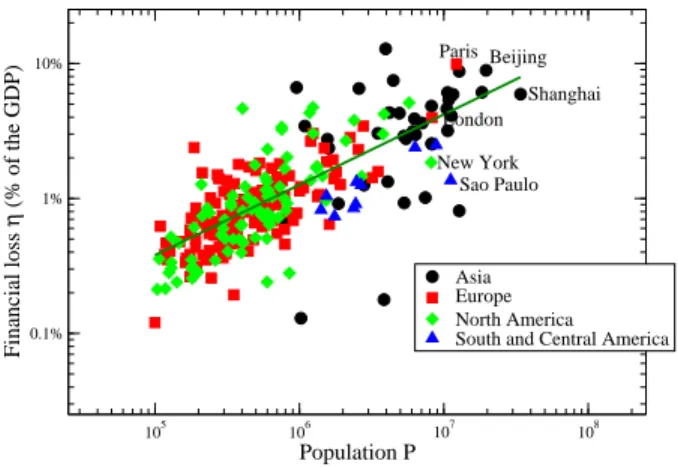
We show this quantity versus population in Figure 2 and we observe a significant increase of this financial loss with population from less than 1% to almost 10% of the
GDP. A power law fit gives a behavior close to η ∼√P
105 106 107 108 Population P 0.1% 1% 10% Financial loss η (% of the GDP) Asia Europe North America South and Central America
Shanghai Beijing Paris London Sao Paulo New York
FIG. 2: Financial loss due to congestion in percent of the gdp per capita (computed for v = 50km/h). The straight line is a power law fit with exponent 0.52 (r2= 0.73).
indicating that even if congestion increases slowly with
population, it generates a non-negligible cost. Asian
cities have a larger loss (on average 4%) followed by the other regions which have roughly the same level (of order 1 − 2%).
There is however a large dispersion around this aver-age behaviour which shows that the population is not the only determinant of this cost. More precisely, for a given value of the population, we observe large differences which probably reflect the efficiency of road infrastruc-tures. We can compute the deviation from the average behavior defined by the power law fit shown in Figure 2 and we observe that in the group of megacities, Paris conjugates both a large income and a high level of con-gestion, while in Sao Paulo average income is low, leading to a relatively small loss. In Beijing, the average income does not compensate the high congestion level, while in London which has a population and an average income of the same order as Paris, we observe an average loss.
What can we conclude from these different observa-tions ? First of all, for the world cities studied in this Tomtom (2016) dataset, congestion obeys a scaling law
3 which seems quite independent from the cultural and
his-torical differences between these cities. Congestion grows – relatively slowly – with the average density and displays an apparent square root behavior. This is the sign that a fundamental mechanism is at play here and begs for some theoretical modeling. In addition, this increase is at odds with the older observation that gasoline consumption de-creases with the average density [16], and suggests that compact development cannot be systematically associ-ated with a decrease in congestion [17]. We thus have contradictory results with respect to density which has an unclear role and this shows that our theoretical un-derstanding of congestion at the urban level, at least, is incomplete. We need more measures and also new theo-retical insights in order to understand the impact of den-sity on congestion, pollution and gasoline consumption. When facing this puzzle, it seems difficult to provide to urban planners and policy makers with good scientific ad-vice which is grounded in observation and theory. How-ever, we understand here that there is at least two factors which play a major role. The first one is obviously the share of individuals travelling to work by car: a decreas-ing share would decrease Ω (but is not likely to change its scaling). Public transportation is a good alternative, especially if it is not too sensitive to congestion. Also, commuting distance is another key factor that governs
the duration of the trip: decreasing τ0 will also decrease
Ω. In some countries (e.g. US, UK, Denmark), this dis-tance is broadly distributed [18] which suggests that we are far from an optimal spatial organization with many mixed land-use centers (such as ‘urban villages’) scat-tered throughout the city.
Thinking about density by itself could thus be very misleading in congestion studies, and it is probably more useful to focus on the spatial redistribution of activities and residences. This could give some clues on how we might reduce the fraction of car users and commuting dis-tances, and how we might develop and encourage health-ier transportation modes.
∗
Electronic address: [email protected]
[1] Anas A, Arnott R, Small KA (1998) “Urban spatial structure” Journal of Economic literature 36(3):1426-1464.
[2] Anas A (2015) “Why are urban travel times so
sta-ble?”Journal of regional science 55:230-261.
[3] DeWeerdt S (2016) “The urban downshift” Nature 531:S52-S53.
[4] Batty M (2013) The New Science of Cities (MIT Press, Cambridge, MA).
[5] Tomtom, traffic congestion index, 2016. http://www. tomtom.com.
[6] Andersen J, Bruwer M (2016) Tomtom 2015 traffic index: independent analysis report (http://www.tomtom. com).
[7] Cox W (2016) “The TomTom traffic index 2015” (http: //www.Tomtom.com).
[8] Pisarski AE (2016) “Tomtom thoughts and observa-tions”, available at: http://www.tomtom.com. [9] Sivak M (2015) “Commuting to work in the 30
largest US cities”, Technical Report, University of Michigan, Transportation Research Institute, available at: https://deepblue.lib.umich.edu/handle/ 2027.42/112057.
[10] Levinson D, and Wu, Y (2005) “The rational locator re-examined: Are travel times still stable?” Transportation 32(2), 187-202.
[11] Louf R, Barthelemy M (2014) “How congestion shapes cities: from mobility patterns to scaling” Scientific Re-ports 4:5561.
[12] United Nations, Statistics Division 2013. Demo-graphic Yearbook 2013. Available at: http: //unstats.un.org/unsd/demographic/
products/dyb/dyb2013.htm
[13] Pumain D (2004) “Scaling laws and urban systems”, Santa Fe Institute Working Paper 2004-02-002, Santa Fe, NM (USA).
[14] Bettencourt LMA, Lobo J, Helbing D, K¨uhnert C, West GB (2007) “Growth, innovation, scaling, and the pace of life in cities” Proceedings of the National Academy of Science, USA 104:7301–7306.
[15] Cox W (2014) “Traffic congestion in the world: 10 worst and best cities”, available at http://www.newgeography.com/content/004504 -traffic-congestion-world-10-worst-and-best -cities.
[16] Newman PW, Kenworthy, JR (1989) “Gasoline consump-tion and cities: a comparison of US cities with a global survey” Journal of the American Planning Association 55(1), 24-37.
[17] Echenique MH, Hargreaves AJ, Mitchell G. Namdeo A (2012) “Growing cities sustainably: does urban form re-ally matter?” Journal of the American Planning Associ-ation 78(2):121-137.
[18] Carra G, Mulalic I, Fosgerau M, Barthelemy M (2016) “Modeling the relation between income and commuting distance” arXiv preprint 1602.01578.