HAL Id: hal-02004120
https://hal-amu.archives-ouvertes.fr/hal-02004120
Submitted on 11 Feb 2020
HAL is a multi-disciplinary open access
archive for the deposit and dissemination of
sci-entific research documents, whether they are
pub-lished or not. The documents may come from
teaching and research institutions in France or
abroad, or from public or private research centers.
L’archive ouverte pluridisciplinaire HAL, est
destinée au dépôt et à la diffusion de documents
scientifiques de niveau recherche, publiés ou non,
émanant des établissements d’enseignement et de
recherche français ou étrangers, des laboratoires
publics ou privés.
Numerical Stiffness Analysis for Solid Oxide Fuel Cell
Real-Time Simulation Applications
Rui Ma, Zhongliang Li, Elena Breaz, Briois Pascal, Fei Gao
To cite this version:
Rui Ma, Zhongliang Li, Elena Breaz, Briois Pascal, Fei Gao. Numerical Stiffness Analysis for Solid
Oxide Fuel Cell Real-Time Simulation Applications. IEEE Transactions on Energy Conversion,
Insti-tute of Electrical and Electronics Engineers, 2018, 33 (4), pp.1917-1928. �10.1109/TEC.2018.2849930�.
�hal-02004120�
Abstract— Real-time simulation is important for the fuel cell online diagnostics and hardware-in-the-loop (HIL) tests before industrial applications. However, it is hard to implement real-time multi-dimensional, multi-physical fuel cell models due to the model numerical stiffness issues. In this paper, the numerical stiffness of a tubular solid oxide fuel cell (SOFC) real-time model is first analyzed to identify the perturbation ranges related to the fuel cell electrochemical, fluidic and thermal domains. Some of the commonly used ordinary differential equation (ODE) solvers are then tested for the real-time simulation purpose. At last, a novel two-stage third-order parallel stiff ODE solver is proposed to improve the stability and reduce the multi-dimensional real-time fuel cell model execution time. To verify the proposed model and the ODE solver, real-time simulation experiments are carried out in a common embedded real-time platform. The experimental results show that the execution speed satisfies the requirement of real-time simulation. The solver stability under strong stiffness and the high model accuracy are also validated. The proposed real-time fuel cell model and the stiff ODE solver can also help to design the online diagnostic control method.
Index Terms—Fuel cell, parallel algorithms, real-time system, stiffness
I. INTRODUCTION
olid oxide fuel cell (SOFC) is one of the solutions to produce electricity via clean and environmentally friendly processes. It is considered as a promising technology for the urban power generation system due to its high fuel efficiency
This work is support by European Commission H2020 grant ESPESA (H2020-TWINN-2015) EU Grant agreement No: 692224; Franche-Comte regional council grant PEMFC aging Regional Grant agreement No: 2013C– 5588/92.
R. Ma is with the Northwestern Polytechnical University, 710072, Xi’an, China, with the Fuel Cell Lab (FCLAB) (FR CNRS 3539), 90010 Belfort, France, and also with the FEMTO-ST (UMR CNRS 6174), Energy Department, Univ. Bourgogne Franche-Comté, UTBM, 90010 Belfort, France (e-mail: [email protected]).
Z. Li is with the LSIS laboratory (UMR CNRS 7296), Aix-Marseille University, 13397 Marseille, France (e-mail: [email protected])
E. Breaz is with the Fuel Cell Lab (FCLAB) (FR CNRS 3539), 90010 Belfort, France, and with the FEMTO-ST (UMR CNRS 6174), Energy Department, Univ. Bourgogne Franche-Comté, UTBM, 90010 Belfort, France, and also with the Technical University of Cluj-Napoca (e-mail: [email protected]).
P. Briois is with FEMTO-ST (UMR CNRS 6174), MN2S Department, Univ. Bourgogne Franche-Comté, UTBM, 25200 Montbéliard, France, (e-mail: [email protected]).
F. Gao is with the Fuel Cell Lab (FCLAB) (FR CNRS 3539), 90010 Belfort, France, and with the FEMTO-ST (UMR CNRS 6174), Energy Department, Univ. Bourgogne Franche-Comté, UTBM, 90010 Belfort, France (e-mail: [email protected]).
and capacity, which draws public concern recently [1]. The SOFC system involves various electrochemical, fluidic, thermal and mechanical phenomena, which makes the optimized control hard to be designed. In order to design efficiently the control strategies of such a complicated multi-physical system and to anticipate eventual system derivation and disturbance during operation, model-based online diagnostic methods should be considered. The real-time simulation is a cost-effective way for system performance test. As known to all that, the real-time modeling accuracy and robustness can influence the online diagnostic and control performance. The use of a high-dimensional (2D or 3D) physical model instead of a low-dimensional (0D or 1D) one can effectively improve the accuracy of the predictive model. By estimating local physical quantities inside the modeled system, a high-dimensional model can enhance the performance of diagnostic control. Since the model can be executed in real-time, the corresponding hardware-in-the-loop (HIL) simulation can also be done without tests on a real fuel cell, which makes the system level tests in a cheaper way. However, the real-time simulation for such a model requires additional efforts due to the fuel cell model inter-coupled stiffness characteristics. Thus, the numerical stiffness brought by the high-dimensional SOFC model should be analyzed to realize real-time applications and optimize its control.
In order to obtain an accurate fuel cell real-time simulation result, a multi-dimensional, multi-physical SOFC model should be built first. Lots of research have attempted to build such models from 2D to 3D [2]-[11]. Although different physical domains, including electrochemical, fluidic and thermal, are considered in the models to predict and estimate local information of the modeled object, these models are all constrained to off-line simulation due to the mathematical complexity or the dependency on the commercial software solution algorithms.
Real-time simulation for fuel cell applications has been raising the research concern recently. However, very few studies are directly related to the multi-dimensional, multi-physical real-time fuel cell models. In [12]-[16], the authors present fuel cell real-time simulation dedicated to the diagnostics and the degradation analysis. Works in [17]-[18] are concentrated on fuel cell power system and energy management applications. The study in [19] contributed to analyzing the ordinary differential equation (ODE) time constants in the fuel cell model. It was found that the time
Numerical Stiffness Analysis for Solid Oxide
Fuel Cell Real-time Simulation Applications
Rui Ma, Student Member, IEEE, Zhongliang Li, Member, IEEE, Elena Breaz, Member, IEEE
Pascal Briois and Fei Gao, Senior Member, IEEE
constants are related to the state-space matrix eigenvalues, which can guide the design of the real-time ODE solver. Massonnat et al. [20] proposed a multi-physical, multi-dimensional real-time proton exchange membrane fuel cell model, in which the current inside the fuel cell is assumed to be distributed uniformly. This can lead to an undesirable error in some applications. Several studies [21]-[23] related to the fuel cell real-time simulation applications failed to deploy a multi-dimensional, multi-physical model. Since 0D approach is used, the fuel cell model proposed by Ramos-Paja et al. [21] has a lower performance when predicting the physical quantities inside the fuel cell. By using dSPACE and Opal-RT platform, a fuel cell real-time simulation model is proposed in [22]. The model performance is compared with different ODE solvers including Euler, 4th order Runge-Kutta (RK4), 5th order Dormand-Prince (DP5) and 4th order Newton extrapolation. Whereas, none of the proposed solvers can meet the requirement of the numerical stiffness variation in a high-dimensional fuel cell model. A 0D fuel cell model for real-time simulation applications on the Opal-RT platform is developed in [23]. The solver used is an embedded solution in the commercial software. Although the commercial software gives the possibility of solving the ODEs for the simulated model, the generated code is often non-optimized to a specific controller. The efficiency of their code generation engines and the embedded solvers are difficult to prove since the software developers usually hold the specific information on how the code has been translated.
It is noticed that real-time simulations of these SOFC models are hard to be realized due to ODE stiffness perturbation under varies model configurations and operating conditions. Thus, it is necessary to analyze the model stiffness variation range and develop a proper ODE solving algorithm to maintain an acceptable performance even under severe stiffness conditions. In this paper, a dynamic, multi-dimensional, multi-physical SOFC model is proposed and applied to the control-oriented real-time simulations based on our previous work [24]. As far as we known, no relevant stiff ODE analysis for a fuel cell model has been discussed in literature before. The major contributions of this paper can be summarized as:
1) The numerical stiffness perturbation caused by the variations of modeling configurations and operating conditions in the multi-dimensional, multi-physical SOFC model is analyzed thoroughly.
2) The performance tests and the effective working range analysis of the most commonly used ODE solvers are conducted for SOFC real-time simulation.
3) A novel two-stage third-order parallel ODE solver is proposed for fuel cell real-time simulation applications. Its high accuracy and robustness are experimentally verified in order to make the SOFC model be executed in real-time.
The rest of the paper is organized as follows: Section II gives the multi-dimensional and multi-physical tubular solid-oxide fuel cell model. The SOFC model covers all three dynamic physical domains including electrochemical, fluidic and thermal domains; Section III is dedicated to the analysis of the model ODE stiffness. The divergence phenomenon is also
discussed when some commonly used ODE solvers are applied to the fuel cell model; in Section IV, the proposed parallel real-time fuel cell ODE solver is developed, and its stability is verified with regard to the deployed model; Section V presents the implementation and the experimental validation of the real-time SOFC model; At last, Section VI concludes this work. II. MULTI-PHYSICAL,MULTI-DIMENSIONAL SOFCMODEL
FOR REAL-TIME SIMULATION
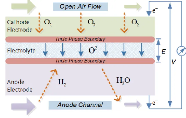
This section presents the governing equations of the multi-physical, multi-dimensional tubular SOFC model in three domains: electrochemical, fluidic and thermal domains. In our developed multi-dimensional model, the finite volume method is applied for spatial discretization. The cell can be divided into N control volumes (CV) along the fuel cell tube axial direction, and four CVs along the tube radial direction: anode channel, anode electrode, electrolyte and cathode electrode. The prototype of SOFC is shown in Fig. 1.
Fig. 1. Tubular SOFC prototype
A. Electrochemical Domain
The polarization curves can be obtained by the output voltage under certain fuel cell currents. The output voltage of the SOFC can be expressed as:
𝐸𝑆𝑂𝐹𝐶= 𝐸𝑟𝑒𝑣− 𝜂𝑎𝑐𝑡,𝑎𝑛− |𝜂𝑎𝑐𝑡,𝑐𝑎| − 𝜂𝑜ℎ𝑚 (1)
where 𝐸𝑟𝑒𝑣 is the SOFC thermodynamic voltage (V), 𝜂𝑎𝑐𝑡,𝑎𝑛
and 𝜂𝑎𝑐𝑡,𝑐𝑎 are the activation loss (V) for anode and cathode,
respectively, 𝜂𝑜ℎ𝑚 represents the electrolyte ohmic loss (V).
It should be noted that the concentration loss is treated implicitly by using directly the gas pressures at catalyst sites.
The thermodynamic voltage 𝐸𝑟𝑒𝑣 represents the maximum
voltage potential that can be derived from reactants to products, which can be obtained through the Nernst equation [24]:
𝐸𝑟𝑒𝑣 = − ∆𝐺0 2𝐹 + 𝑅𝑇 2𝐹ln ( 𝑃H2√𝑃O2 𝑃H2O ) (2)
where ∆𝐺0 is the Gibbs free energy change in the oxidations
(J/mol), 𝑇 is the temperature at the reaction site (K), 𝑃H2, 𝑃H2O
and 𝑃O2 are the gas pressures at the triple phase boundary (TPB)
(atm), F = 96485.3 is the Faraday constant (C/mol), and R = 8.314 is the ideal gas constant (J/(mol·K)).
The static activation voltage loss 𝜂𝑎𝑐𝑡 can be expressed by
𝑖 = 𝑗0𝐴𝑒𝑙[exp ( 𝛼𝑛𝑒𝐹
𝑅𝑇 𝜂𝑎𝑐𝑡) −exp ( 𝛽𝑛𝑒𝐹
𝑅𝑇 𝜂𝑎𝑐𝑡)] (3)
where i is the current of the fuel cell (A), 𝐴𝑒𝑙 is the area of the
electrode (m2), 𝑗
0 is the exchange current density (A/m2), 𝑛𝑒 is
the electrons number involved in the half reactions at anode or cathode, 𝛼, 𝛽 are symmetry factors.
The ohmic loss is caused by the yttria-stabilized zirconia (YSZ) electrolyte resistance, which can be calculated as:
𝜂𝑜ℎ𝑚= 𝑖 ∙ 𝛿𝑌𝑆𝑍
𝐴𝑒𝑙𝜎𝑌𝑆𝑍 (4)
where 𝜎𝑌𝑆𝑍 is the YSZ electrical conductivity (S·K/m), 𝐴𝑒𝑙 is
the electrolyte area (m2) , 𝛿
𝑌𝑆𝑍 is the electrolyte thickness (m).
Due to the double layer capacitances effects on the fuel cell anode and cathode, the dynamic activation loss can be given in the form of:
d dt𝑉𝑎𝑐𝑡 = 𝑖 C𝑑𝑙(1 − 1 𝜂𝑎𝑐𝑡𝑉𝑎𝑐𝑡) (5)
where 𝑉𝑎𝑐𝑡 is the dynamic activation loss (V), 𝐶𝑑𝑙 represents
the fuel cell double layer capacitance for anode and cathode (F).
B. Fluidic Domain
The fuel gas flows into the anode tube channel along the axial direction, and the diffusion in the solid phase is caused by concentration gradient at the two sides of the electrodes. The SOFC fluidic pressure dynamic response in the channel can be described by the mass conservation differential equation:
d dt𝑃𝑔𝑎𝑠,𝑐ℎ= 𝑅𝑇 𝑀𝑔𝑎𝑠𝑉𝑐ℎ∙ ∑ 𝑞𝑔𝑎𝑠 𝑐ℎ 𝑖𝑛/𝑜𝑢𝑡 (6)
where 𝑉𝑐ℎ is the volume of the channel (m3), 𝑀𝑔𝑎𝑠 is the fuel
gas molar mass (kg/mol), 𝑃𝑔𝑎𝑠,𝑐ℎ is the gas pressure in the
anode channel (Pa), and 𝑞𝑔𝑎𝑠 represents the molar gas flowrate
entering and leaving the anode channel (kg/s).
The reacted gas diffusion in the Gas Diffusion Layer (GDL) is directly related to SOFC current, which can be expressed as:
𝑞𝑔𝑎𝑠,𝐺𝐷𝐿= 𝑖
𝑛𝑒𝐹 (7)
During the SOFC operation, the gas flow contains not only hydrogen and vapor but also Argon gas in the case of our experiments. The diffusion of certain species among the mixed gas in the solid phases can be expressed by the Stefan-Maxwell equation [24]: ∆𝑃𝑖= 4𝑅𝑇𝛿𝐺𝐷𝐿 𝜋𝑃𝑓𝑢𝑒𝑙𝐷𝑐ℎ2∑ 𝑃𝑖(𝑞𝑗/𝑀𝑗)−𝑃𝑗(𝑞𝑖/𝑀𝑖) 𝐷𝑖𝑗 𝑖≠𝑗 (8)
where 𝑃𝑓𝑢𝑒𝑙 is the total pressure of the fuel gas in the electrode
(Pa), δGDL is the electrode thickness (m), 𝐷𝑐ℎ represents the
tube hydraulic diameter (m), 𝑃𝑖 and 𝑃𝑗 stand for the gas
pressures of specie i and j (Pa), respectively, 𝑞𝑖 and 𝑞𝑗 are the
molar gas flowrates (kg/s), 𝑀𝑖 and 𝑀𝑗 represent the gas molar
mass of (kg/mol) and 𝐷𝑖𝑗 is the binary diffusion coefficient
(m2/s).
The binary diffusion coefficient can usually be described by the Slattery-Bird equation [24]:
𝐷𝑖𝑗= 𝑎 𝑃𝑔𝑎𝑠( 𝑇 √𝑇𝑐,𝑖∙𝑇𝑐,𝑗) 𝑏 (𝑃𝑐,𝑖𝑃𝑐,𝑗) 1 3⁄ (𝑇𝑐,𝑖𝑇𝑐,𝑗) 5 12⁄ (10−3 𝑀𝑖 10−3 𝑀𝑗) 1 2⁄ (9) where temperature 𝑇𝑐 and pressure 𝑃𝑐 represent the critical
value for certain gas species. For bipolar gas species,𝑎 = 2.745 × 10⁻⁴ , 𝑏 = 1.823 , otherwise for un-bipolar gas
species, 𝑎 = 3.640 × 10⁻⁴, 𝑏 = 2.334.
C. Thermal Domain
Thermal analysis of SOFC plays an important role in fuel cell diagnostics and predictive control. Reaction temperatures, which vary from 973.15 K to 1173.15 K, can impose non-negligible thermal stress due to the different thermal expansion coefficients of the SOFC materials. Thus, an accurate thermal dynamic model is necessary to reveal the temperature distribution inside of the SOFC.
1) Electrode-electrolyte solid phase thermal dynamics
The thermal dynamics for the electrode-electrolyte solid phase include the conduction heat, forced convection heat, mass convection heat and internal heat sources. The governing equation is given as:
(𝜌𝑠𝑜𝑙𝑖𝑑𝑉𝑠𝑜𝑙𝑖𝑑𝐶𝑠𝑜𝑙𝑖𝑑) d
dt𝑇𝑠𝑜𝑙𝑖𝑑= 𝑄𝑚+ 𝑄𝑓𝑐+ 𝑄𝑐𝑑+ 𝑄𝑖𝑛𝑡 (10)
where 𝑇𝑠𝑜𝑙𝑖𝑑 is the temperature of the solid phase CV (K),
𝜌𝑠𝑜𝑙𝑖𝑑 is the solid phase density (kg/m3), 𝑉𝑠𝑜𝑙𝑖𝑑 represents the
volume for the solid phase CV (m3), 𝐶
𝑠𝑜𝑙𝑖𝑑 is the thermal
capacity (J/(kg·K)), 𝑄𝑐𝑑 is the conduction heat which describes
the heat transfer between the solid phases (J/s), 𝑄𝑖𝑛𝑡 represents
the internal heat sources including resistive loss, activation loss and irreversible electrochemical loss (J/s).
The fuel gas species diffuse into or out of certain CV in solid phase can lead to mass convection heat expressed as:
𝑄𝑚= ∑𝑠𝑝𝑒𝑐𝑖𝑒𝑠𝑞𝑔𝑎𝑠𝑀𝑔𝑎𝑠𝐶𝑔𝑎𝑠,𝑠𝑝(𝑇𝑎𝑚𝑏− 𝑇𝑠𝑜𝑙𝑖𝑑) (11)
where 𝐶𝑔𝑎𝑠,𝑠𝑝 is the thermal capacity for the fuel gas species in
the solid phase (J/(kg·K)), 𝑇𝑎𝑚𝑏 and 𝑇𝑠𝑜𝑙𝑖𝑑 are the temperature
for the ambient and current CV (K), respectively.
The forced convection describes the heat transfer between the anode channel fuel gas flow and the inner surface of the solid phase, which can be expressed as:
𝑄𝑓𝑐= ℎ𝑓𝑐𝐴𝑠𝑜𝑙𝑖𝑑(𝑇𝑐ℎ𝑙− 𝑇𝑠𝑜𝑙𝑖𝑑) (12)
where 𝑇𝑐ℎ𝑙 is the channel fuel gas temperature (K), ℎ𝑓𝑐 is the
forced convection coefficient (W/(m2·K)), 𝐴
𝑠𝑜𝑙𝑖𝑑 represents the
surface area between anode channel and the solid phase (m2).
Conduction heat between different CVs can be obtained through the Fourier heat transfer equation as:
𝑄𝑐𝑑= ∑
𝜑𝑠𝑜𝑙𝑖𝑑𝐴𝑐𝑜𝑛𝑡
𝛿𝑠𝑜𝑙𝑖𝑑
𝐶𝑉 (𝑇𝑎𝑚𝑏− 𝑇𝑠𝑜𝑙𝑖𝑑) (13)
where 𝜑𝑠𝑜𝑙𝑖𝑑 is the thermal conductivity of the solid phase
(W/(m·K)), 𝐴𝑐𝑜𝑛𝑡 is the contact area between different CVs
(m2), 𝛿
𝑠𝑜𝑙𝑖𝑑 is the thickness for the current solid phase CV (m).
The last term on the right side of (10) represents the internal heat sources, which can be obtained as:
𝑄𝑖𝑛𝑡 = 𝑖 (𝑉𝑎𝑐𝑡,𝑎𝑛+𝑉𝑎𝑐𝑡,𝑐𝑎+ 𝜂𝑜ℎ𝑚− 𝑇𝑠𝑜𝑙𝑖𝑑𝑆0
where 𝑆0 is the entropy change from the reactants to products
(J/(mol·K)).
2) Channel fluidics thermal dynamics
The fuel gas fluidics in the anode channel is related to mass flow convection along the anode channel and forced convection between anode channel fuel gas and the solid phase inner surface. The governing differential equation can be given as:
(𝜌𝑔𝑎𝑠𝑉𝑔𝑎𝑠𝐶𝑔𝑎𝑠) d
dt𝑇𝑐ℎ𝑎𝑛𝑙= 𝑄𝑚+ 𝑄𝑓𝑐 (15)
where 𝜌𝑔𝑎𝑠 is the density of the fuel gas flow (kg/m3), 𝑉𝑔𝑎𝑠 is
the volume of the anode channel CV (m3), 𝐶
𝑔𝑎𝑠 is the average
thermal capacity for the gases in the anode channel (J/(kg·K)). III. ODESTIFFNESS PERTURBATION IN SOFCREAL-TIME
SIMULATION
In this section, the obtained ordinary differential equations (ODEs) stiffness perturbation range of the SOFC model is discussed. Several ODE solvers are applied to the SOFC model for evaluating performances under stiffness.
A. Stiffness Perturbation 1) ODE Stiffness Definition
To solve numerically the developed dynamic SOFC model, all the ODEs should be arranged firstly into a state-space of dimension n:
d
dt𝒙⃗⃗ = 𝑨 ∙ 𝒙⃗⃗ + 𝒇(𝑡) (16)
where 𝑨 is a matrix of dimension n with the eigenvalues 𝜆1, 𝜆2, ⋯ , 𝜆𝑛, 𝒙⃗⃗ is the state-variable vector. If the physical
quantities of the model are with different time scales, i.e. different values of 𝜆, the stiff problem will occur when
𝛤 =max(|𝑅𝑒(𝜆)|)
min(|𝑅𝑒(𝜆)|)≫ 1 (17)
where 𝛤 is the stiffness of the system.
2) SOFC Stiffness Discussion
For the proposed multi-dimensional, multi-physical SOFC real-time model, strong stiffness exists in each individual physical domain, and also in-between the different domains, since the parameters are all inter-coupled. In order to simplify the analysis, the thermal dynamic characteristics in the model are chosen as the analyzing object. The prototype of the proposed real-time SOFC model control volumes can be seen in Fig. 2.
Fig. 2. A prototype of the real-time tubular SOFC control volume
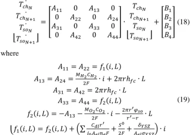
The SOFC can be divided into individual CVs along the tube axial direction, and the thermal dynamic performance for each CV is analyzed in-between the solid-phases and anode channel. In order to quantify the stiffness of the real-time fuel cell model, (10) and (15) can be arranged into state-space form for the two adjacent CVs in Fig.2 as:
[ 𝑇𝑐ℎ̇𝑁 𝑇𝑐ℎ𝑁+1 𝑇𝑠𝑜̇𝑁 𝑇𝑠𝑜𝑁+1̇ ̇ ] = [ 𝐴11 0 𝐴13 0 0 𝐴22 0 𝐴24 𝐴31 0 𝐴33 0 0 𝐴42 0 𝐴44 ] ∙ [ 𝑇𝑐ℎ𝑁 𝑇𝑐ℎ𝑁+1 𝑇𝑠𝑜𝑁 𝑇𝑠𝑜𝑁+1] + [ 𝐵1 𝐵2 𝐵3 𝐵4 ] (18) where { 𝐴11= 𝐴22= 𝑓1(𝑖, 𝐿) 𝐴13= 𝐴24= 𝑀𝐻2𝐶𝐻2 2𝐹 ∙ 𝑖 + 2𝜋𝑟ℎ𝑓𝑐∙ 𝐿 𝐴31= 𝐴42= 2𝜋𝑟ℎ𝑓𝑐∙ 𝐿 𝐴33= 𝐴44= 𝑓2(𝑖, 𝐿) 𝑓2(𝑖, 𝐿) = −𝐴13− 𝑀𝑂2𝐶𝑂2 2𝐹 ∙ 𝑖 − 2𝜋𝑟′𝜑𝑠𝑜 𝑟′−𝑟 ∙ 𝐿 𝑓1(𝑖, 𝐿) = 𝑓2(𝑖, 𝐿) + (∑ 𝐶𝑑𝑙𝑟′ 𝑗0𝐴𝑒𝑙𝑛𝑒𝐹+ 𝑆0 2𝐹+ 𝛿𝑌𝑆𝑍 𝐴𝑒𝑙𝜎𝑌𝑆𝑍) ∙ 𝑖 (19)
where temperatures 𝑇𝑐ℎ and 𝑇𝑠𝑜 are of channel side and solid
phase, respectively, 𝑟′ is the tube outer radius (m), r is the
channel inner radius (m), L is the length for each CV (m). As it can be seen from (19), all the parameters in the state matrix A are related to the fuel cell current and the individual CV length. By considering (9), (13) and (14), the coupled relationship among electrochemical, fluidic and thermal domains can be revealed: the mass molar flow rate in the GDL can be obtained through (9), and the conduction heat term is related to the CV length as (13), whereas the internal heat source term (14) in the thermal dynamic equations is a function of the fuel cell current. Then the eigenvalue of thermal dynamic model matrix A can be calculated through (20).
det(𝜆𝑰 − 𝑨) = | 𝜆 − 𝐴11 0 −𝐴13 0 0 𝜆 − 𝐴22 0 −𝐴24 −𝐴31 0 𝜆 − 𝐴33 0 0 −𝐴42 0 𝜆 − 𝐴44 | = 0 (20)
A solution of (20) is calculated and shown in (21). The eigenvalues of thermal dynamics in the SOFC model can then be obtained for real-time model stiffness perturbation range analysis under varying modeling and operating conditions.
{ 𝜆1= 1 2(𝐴11+ 𝐴33− (𝐴11 2− 2𝐴 11𝐴33+ 𝐴332+ 4𝐴13𝐴31) 1 2) 𝜆2=12(𝐴22+ 𝐴44− (𝐴222− 2𝐴22𝐴44+ 𝐴442+ 4𝐴24𝐴42) 1 2) 𝜆3=12(𝐴11+ 𝐴33+ (𝐴112− 2𝐴11𝐴33+ 𝐴332+ 4𝐴13𝐴31) 1 2) 𝜆4= 1 2(𝐴22+ 𝐴44+ (𝐴22 2− 2𝐴 22𝐴44+ 𝐴442+ 4𝐴24𝐴42) 1 2) (21)
Table I gives the stiffness perturbation when the modeling control volume numbers change. The tests are conducted under 0.5 A fuel cell current and with 59.22% of H2 and 19.74% of
H2O as input fuel gas. The experimental temperature for the
when more modeling CVs are considered for the multi-dimensional, multi-physical SOFC, the model stiffness increases dramatically due to a smaller distance between individual CVs is applied to the model.
TABLEI
MODEL CONTROL VOLUME NUMBERS AND STIFFNESS TESTS
Control Volume Number SOFC Model |𝜆𝑚𝑖𝑛| SOFC Model |𝜆𝑚𝑎𝑥| SOFC Model Stiffness 1 0.0229 110.33 4817.90 2 0.0184 149.69 6536.68 5 0.0126 269.58 11772.05 10 0.0096 467.33 20407.42 20 0.0076 867.57 37885.15 50 0.0063 2060.19 89964.63 100 0.0013 18355.18 801536.24 200 0.0012 36645.53 1600241.48
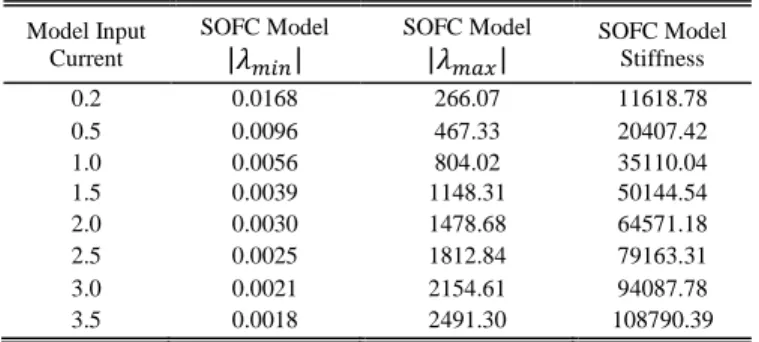
Table II gives the stiffness perturbation under different fuel cell input currents with 10 modeling CVs along the axial direction. This group is tested under 1123.15 K with the same fuel gas molar fractions in the previous test. Compared with the variation caused by CV numbers in the last test, the influence brought by input current variation is smaller.
TABLEII
MODEL INPUT CURRENT AND STIFFNESS TESTS
Model Input Current SOFC Model |𝜆𝑚𝑖𝑛| SOFC Model |𝜆𝑚𝑎𝑥| SOFC Model Stiffness 0.2 0.0168 266.07 11618.78 0.5 0.0096 467.33 20407.42 1.0 0.0056 804.02 35110.04 1.5 0.0039 1148.31 50144.54 2.0 0.0030 1478.68 64571.18 2.5 0.0025 1812.84 79163.31 3.0 0.0021 2154.61 94087.78 3.5 0.0018 2491.30 108790.39
In real-time simulations, the ODE solver working range is related to the model stiffness. It can be concluded, from the above two group tests, that the SOFC model stiffness can have a large variation range under different modeling configurations and operating conditions.
It should be noted that, the time-step in microseconds range can usually be found in the real-time simulation for the power electronic models. This is because the high frequency behavior of the power components, such as MOSFET or IGBT, need to be simulated in real-time, and simulation time-step should be at least ten times smaller compared with the switching period and the sampling time. However, in the case of the multi-physical fuel cell model, the time constants in electrochemical, fluidic and thermal domains can vary a lot, and can be of several orders of magnitude bigger than the time constants in the power electronic models. Thus, the simulation time step is usually chosen to be in millisecond range for a multi-dimensional multi-physical fuel cell model.
B. ODE Solvers tests for Real-time Simulation
The ODE solver performance for the real-time simulation is very important for the stability and the accuracy of the executed
model. The configuration of the solver time step, the modeling configurations, and the operating conditions can all influence the performance. Some most commonly used ODE solvers are tested and discussed with regard to the real-time SOFC model in this part.
1) Euler Forward Method (1st order)
The Euler forward method is applied to the real-time SOFC model for testing the stability firstly. As it can be seen from Fig. 3, the simulation time step is set to h = 2.3 ms, with the horizontal axis denoting the calculated time steps. The electrolyte temperature at the inlet part (first axial control volume) of the fuel cell tube remains stable within 20 CVs configuration under a 0.5 A step current input change, whereas the temperature curves become unstable when the modeling CV number gradually increases from 21 to 25.
Fig. 3. SOFC electrolyte temperature with Euler method
The absolute stability region of the forward Euler method can be expressed as:
|1 + ℎ ∙ 𝜆| ≤ 1 (22)
The model stable region of the eigenvalues can be then obtained by applying the value of time step into (22) as:
−869.56 ≤ 𝜆 ≤ 0 (23)
The result corresponds with the SOFC model stiffness calculated in Table I very well. Clearly, the forward Euler method is not suitable for the proposed multi-dimensional real-time SOFC model under a large number of modeling CVs.
2) Trapezoidal Method (2nd order)
Trapezoidal method is a second order implicit numeric method, which is widespread for solving ODEs due to the stable characteristic without any requirement:
|(2 + ℎ ∙ 𝜆)
(2 − ℎ ∙ 𝜆)| ≤ 1 (24)
The numerical stability of a solver is directly related to the eigenvalues λ of the ODEs to be solved, with Re(λ)<0 for most of the engineering problems. It can be seen from (24) that trapezoidal method is stable regardless of the time step value. However, the iteration in each time step is time-consuming.
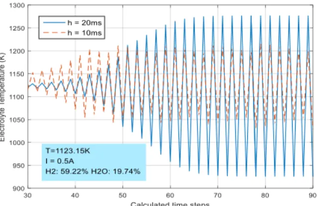
Fig. 4 shows the SOFC electrolyte temperature at the inlet part (first axial control volume) of the fuel cell tube solved by trapezoidal method under 25 CVs configuration. The
simulation time steps are set to h = 10 ms and h = 20 ms, respectively. The temperature dynamic response to a 0.5 A step current change ends in oscillations without convergence. A smaller time step can have a lower oscillation altitude. The stability can be satisfied (i.e. no divergence) whereas no accuracy can be ensured.
Fig. 4. SOFC electrolyte temperature with trapezoid method
IV. DEVELOPMENT OF REAL-TIME SOFCMODEL PARALLEL
ODESOLVER
It can be seen from the previous section that the ODE stiffness varies a lot under different modeling configurations and operating conditions. The required modeling performance under strong stiffness cannot be satisfied by using the commonly used solvers. It is thus necessary to deploy an effective algorithm to alleviate the effect of ODE stiffness and improve the performance of the fuel cell real-time simulation. In this section, a parallel algorithm is proposed and applied to the multi-dimensional SOFC real-time model.
A. Stiff ODE Parallel Algorithm Design
The commonly used ODE solvers presented in the previous section can all be executed in real-time, whereas the convergence cannot be attained under a serious stiffness condition. In order to increase the robustness of the algorithm, stiff ODE solver should be introduced. However, stiff ODE solvers proposed in the literature usually require solving nonlinear implicit equations, and Newton iteration methods used for solving these equations take lots of computing time which are not desired in real-time simulation [25]. For example,
s-stage implicit Runge-Kutta method applied for solving a m-order ODEs requires solving a 𝑠 × 𝑚 -order nonlinear implicit equations in every integral step. To decrease the computing time, Rosenbrock proposed a new ODE solver which only requires solving linear equations instead of the nonlinear ones [26].
Rosenbrock method can be easily programmed and implemented to the embedded applications like real-time simulation. However, the calculating of the intermediate time step values consumes lots of time. For the multi-dimensional multi-physical fuel cell model, conventional Rosenbrock [26] method may lead to overrun when a large CV number is confronted. Thus, a class of real-time parallel extended Rosenbrock methods is developed for the proposed fuel cell
model in this paper to realize real-time simulation as:
{
(𝑰 − ℎ𝛾𝑖𝑖𝑱)𝑘𝑖𝑛= ℎ𝑓(𝑦𝑛+ ∑𝑠𝑗=1𝜔𝑖𝑗𝑘𝑗,𝑛−1)
+ℎ𝑱 ∑𝑠𝑗=1𝜒𝑖𝑗𝑘𝑗,𝑛−1, 𝑖 = 1, 2, ⋯ , 𝑠
𝑦𝑛+1= 𝑦𝑛+ ∑𝑠𝑖=1𝜙𝑖𝑘𝑖𝑛
(26)
where ℎ > 0 is the integration step size, 𝛾𝑖𝑖, 𝜔𝑖𝑗, 𝜙𝑖, 𝜒𝑖𝑗 are real
coefficients, I represents the identity matrix, J is the Jacobian matrix, 𝑦𝑛 is an approximation to y(𝑡𝑛) and 𝑘𝑖𝑛 here indicates
an approximation to some information of 𝑘𝑖(𝑡𝑛, ℎ) about the
exact solution y(𝑡).
Since the quantities 𝑦𝑛, 𝑘1,𝑛−1, 𝑘2,𝑛−1, ⋯ , 𝑘𝑠,𝑛−1 are known,
𝑘1,𝑛, 𝑘2,𝑛, ⋯ , 𝑘𝑠,𝑛 can be calculated on s different processors in
a parallel way. The proposed method can sufficiently increase the parallel efficiency because the internal stage values are only depending on the numeric values in previous step. Thus, the fuel cell model can be executed in real-time when large CV numbers is applied. Fig. 6 shows the structure of the solving algorithm executed by two processors.
n
y
y
n1 Processor 1 Processor 2 1 , 1n k 1 , 2n k 1 k 2 kFig. 5. Structure of the solving algorithm
By considering the two-stage third-order solving algorithm, the order condition equations can be expressed as:
{ ∑2𝑗=1𝜙𝑗= 1, ∑ 𝜙𝑗𝑝𝑗 = 1 2 2 𝑗=1 , ∑ 𝜙𝑗𝑞𝑗= 1 6 2 𝑗=1 𝑞𝑖= 1 2(∑ 𝜔𝑖𝑗 2 𝑗=1 ) 2 , 𝑝𝑖= ∑2𝑗=1(𝜔𝑖𝑗+ 𝜒𝑖𝑗) + 𝛾𝑖𝑖 𝑞𝑖= ∑𝑗=12 (𝜔𝑖𝑗+ 𝜒𝑖𝑗)(𝑝𝑗− 1) + 𝛾𝑖𝑖𝑝𝑖, 𝑖 = 1,2 𝜙𝑖= ∑2𝑗=1𝜙𝑖𝑗, 𝑖 = 1,2 (27)
Thus the proposed parallel algorithm contains seven free parameters: 𝜙1, 𝜙2, 𝛾11, 𝛾22, 𝜒11, 𝜒12, 𝜙22. Through the Powell
method [27], an optimized group of parameters can be obtained for the strong robustness of the parallel extended Rosenbrock method as: { 𝜙1= 1 2, 𝜙2= 1 𝛾11= 4 5, 𝛾22= 8 5 𝜒11= 𝜒22= 𝜙12= 0 (28)
The corresponding two-stage third-order real-time parallel extended Rosenbrock method can thus be expressed as:
{ (𝑰 −4 5ℎ𝑱) 𝑘1𝑛= ℎ𝑓 (𝑦𝑛+ 169 480𝑘1,𝑛−1+ 71 480𝑘2,𝑛−1) (𝑰 −8 5ℎ𝑱) 𝑘2𝑛= ℎ𝑓(𝑦𝑛+ 𝑘1,𝑛−1) +ℎ𝑱 (−4901 720𝑘1,𝑛−1+ 1219 720𝑘2,𝑛−1) 𝑦𝑛+1= 𝑦𝑛+ 8 9𝑘1𝑛+ 1 9𝑘2𝑛 (29)
B. Numerical Stability Analysis
For investigating the numerical stability of the proposed algorithm, the real-time parallel extended Rosenbrock method can be applied to the scalar test equation as:
𝑑𝑦(𝑡) 𝑑𝑡 = 𝑓(𝑡, 𝑦(𝑡)) = 𝜆𝑦⁄ (30) Thus we can obtain
𝑦𝑛+1= 𝑀(𝑧)𝑦𝑛 (31)
where 𝑧 = ℎ𝜆, the stability matrix is
𝑀(𝑧) = ( 169𝑧 480(1−45𝑧) 71𝑧 480(1−45𝑧) 𝑧 480(1−45𝑧) −4181𝑧 720(1−8 5𝑧) −1219𝑧 720(1−8 5𝑧) 𝑧 720(1−4 5𝑧) −2153𝑧+500𝑧2 6480(1−4 5𝑧) −367𝑧+1940𝑧2 6480(1−4 5𝑧) 9−63 5𝑧+ 52 25𝑧2 9(1−4 5𝑧) ) (32)
with the characteristic polynomial Λ(𝜉, 𝑧) = 𝜉3+𝑁2(𝑧) 𝑁3(𝑧)𝜉 2+𝑁1(𝑧) 𝑁3(𝑧)𝜉 + 𝑁0(𝑧) 𝑁3(𝑧) (33) where { 𝑁0(𝑧) = −0.26𝑧2+ 0.61𝑧3− 0.43𝑧4 𝑁1(𝑧) = −1.34𝑧 + 3.32𝑧2− 2.27𝑧3+ 0.58𝑧4 𝑁2(𝑧) = −1 + 5.14𝑧 − 6.46𝑧2+ 0.15𝑧3+ 1.79𝑧4 𝑁3(𝑧) = 1 − 4.80𝑧 + 8.32𝑧2− 6.14𝑧3+ 1.63𝑧4 (34)
By using the boundary locus methods and employing Schur criterion [28], the roots for characteristic polynomial Λ(𝜉, 𝑧) = 0 can be obtained as:
|𝜉(𝑧)| < 1, 𝑅𝑒(𝑧) < 0 (35) Thus the proposed two-stage third-order real-time parallel extended Rosenbrock method is A-stable.
C. Algorithm Validations
In order to verify the accuracy and convergence of previous stiff ODE solvers and the proposed one, offline simulation tests are conducted first. The temperature of the electrolyte is used to verify the performance. By setting different values of the simulation time step, modeling CV numbers and fuel cell operating conditions, the comparisons between different ODE solvers can be made.
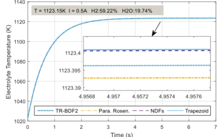
Specifically, as shown in Fig. 6, the tests are first conducted under lower stiffness with 25 CVs for the fuel cell model. The reaction fuel gas molar fractions of H2 and H2O are 59.22% and
19.74%, respectively. The electrolyte temperature dynamic responses to a 0.5 A step current input are simulated. Despite previous mentioned Trapezoidal Method, the simulation under Numerical Differentiation Formulas (NDFs) Method and Trapezoidal Rule with the second order Backward Difference Formula (TR-BDF2) are also compared with the Rosenbrock method. In this group tests, the proposed solver has a fixed simulation time step of 10 ms, whereas other solvers are simulated under variable steps mode. It can be seen from the figure that the numerical accuracy of the tested solvers is almost the same when the solver solution is in the stable region.
The result obtained from Rosenbrock method shows the same level of numerical accuracy compared with other numerical methods.
Fig. 6. Stiff solver accuracy comparisons (25 CVs)
Furthermore, in order to show clearly the superior performance of the proposed solver in the numerical stiff cases, the solver's offline performance under a higher modeling stiffness are shown in the following Fig. 7. When a small simulation time step is applied to the trapezoidal method, the temperature response to a 2.5 A step current input is similar to the results simulated by Rosenbrock method. However, when the simulation time step increases, the numerical oscillations can be observed in the temperature using trapezoidal method, and the solver failed to converge.
Fig. 7. Stiff solver stability comparisons(25 CVs)
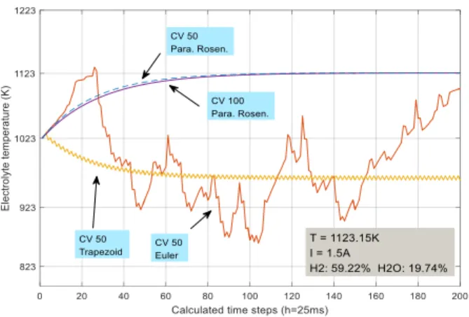
Then, the two-stage third-order real-time parallel extended Rosenbrock method is applied to the model with strong stiffness in order to verify its performance. The tests are conducted with modeling CV numbers of 50 and 100 respectively, with the fuel gas composition of 59.22% H2, 19.74% H2O. As it can be seen from Fig. 8, the temperature of the electrolyte at the fuel cell tube inlet part can converge numerically under a 1.5A step current input with proposed methods, whereas other methods include Euler Midpoint Method and Trapezoidal Method failed to reach stable under such a high stiffness modeling condition.
It can be concluded from the above offline simulation results that the proposed parallel extended Rosenbrock method is numerically robust under both weak and strong numerical ODE
stiffness. The stability and high accuracy make it capable to solve the multi-dimensional multi-physical fuel cell model in real-time.
Fig. 8. SOFC electrolyte temperature dynamic response
V. REAL-TIME SOFCMODEL IMPLEMENTATION AND
EXPERIMENTAL VALIDATION
A. Real-time Model Execution Flowchart
With the developed multi-dimensional, multi-physical fuel cell model and the A-stable parallel stiff ODE solver, the performance of the real-time SOFC model can be verified through the simulations and experimental tests. Fig. 9 gives the model execution flowchart.
The real-time model input parameters include the fuel cell current, the environmental temperature, and the fuel gas pressure along with the species molar fraction. Before the real-time simulation, the governing equations for the fuel cell need to be arranged into state-space equations form. Then the entire model is coded and implemented to the commercial Opal-RT 3.4 GHz QNX-based real-time simulator platform. Since the main focus of this work is the stiffness analysis in the multi-dimensional multi-physical SOFC model, the proposed real-time model and stiff ODE solver consist of the fuel cell itself without consideration of other systems components. Thus, in the simulated model, no other systems and components are modeled. The processor can reach the real-time simulation requirements of the proposed complex multi-dimensional, multi-domain tubular SOFC model. The performance of the algorithm will be verified regarding the model execution time.
Fig. 9. Real-time SOFC model execution flowchart
B. Experimental Setup and Model Benchmark tests
The input fuel gas for the modeled SOFC contains a mixture gas of H2 and H2O. In addition, argon gas is added to maintain
the total gas pressure in the anode channel when individual gas partial pressure varies. During the experimental tests, the molar fractions of dry hydrogen and argon gas are controlled by the flow valves. The water is pumped into the heated vaporizer cylinder in order to be mixed with the input fuel gas. The cathode side of the fuel cell is exposed to the heated airflow within the furnace, and the temperature is assumed to be uniformly distributed. The physical quantities, i.e. current and voltage, can be obtained through the electronic load. The prototype for the experimental setup of the fuel cell test bench is shown in Fig. 10.
Hydrogen
Controlled water pump
SOFC Water Argon Heated gas supply line Electronic load Exhaust (gas recycle) Vaporizer Flow controller Flow controller Opal-RT Simulator Embedded real-time SOFC model
Data
Fig. 10. A prototype of the real-time SOFC experimental setup
Table III shows the real-time model benchmark results under different number of SOFC control volumes along the axial direction. When there is only one modeling CV, the solver execution time represents the solver computation time plus the algebraic equations computation time. It can be seen from the table that the overall real-time simulation time steps for the strong numerical stiff SOFC model can reach the millisecond level without overrun.
TABLEIII
REAL-TIME SOFCMODEL BENCHMARK PERFORMANCE
Control Volume Number Model CPU execution time Model time step set up 1 1.201ms 1.5ms 2 2.435ms 2.5ms 5 6.594ms 7ms 10 14.676ms 15ms 20 28.853ms 30ms 50 58.026ms 60ms 100 124.505ms 130ms 200 252.467ms 260ms
C. Real-time Model Validation
The polarization curves obtained by real-time SOFC model and experimental tests under different temperatures and various fuel gas species molar fraction are shown in Fig. 11 to Fig. 14, It can be seen that the real-time simulation results correspond very well the experimental results within a relative error of 3.46%. A higher H2 fraction will lead to higher thermodynamic
voltage. Under the same fuel fraction and cell current, a higher reaction temperature will lead to a higher voltage. Through monitoring the operating conditions continually, the behavior of the SOFC can be effectively simulated in real-time.
Specifically, as shown in Fig. 11, the real-time simulation for the fuel cell model is conducted under 19.74% H2O and 35.53% H2. The temperatures vary from 1023.15 K to 1123.15 K. It can
be seen from the figure that the real-time simulation results fit the experimentally measured fuel cell polarization data very well. It can be concluded that the polarization performance of the fuel cell can be influenced by temperature greatly.
Fig. 11. Real-time SOFC polarization curves
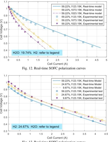
Another group of real-time simulations is conducted under a higher molar fraction of H2. As shown in Fig. 12, under the
same fuel cell current, a lower reaction temperature will lead to a lower fuel cell voltage. The errors between the real-time simulation results and the experimentally measured data are very small, which indicate the real-time model can reach a high accuracy.
Fig. 12. Real-time SOFC polarization curves
Fig. 13. Real-time SOFC polarization curves
Moreover, the performance of the real-time model under varies fuel gas molar fraction is tested. In this group of tests, the molar fraction of H2 is set to 24.67%, whereas the fraction of H2O varies from 9.87% to 59.22%. It can be seen from Fig. 13
that the real-time simulation results fit the measured data well. A higher H2O fraction will lead to lower thermodynamic voltage.
Compared to the fuel cell operating temperature in Fig. 13, a lower temperature of 1073.15 K is applied to the real-time simulation. As shown in Fig. 14, the real-time modeling results can also fit the experimentally measured polarization data well. However, it can be noticed that under the same fuel cell current, a lower fuel cell voltage can be found in Fig. 14 when compared with Fig. 13.
Fig. 14. Real-time SOFC polarization curves
Fig. 15 presents the anode channel gas fuel pressure distribution in the real-time SOFC model. This group is tested under 1073.15 K, with the same molar fraction of H2 and vapor
as 24.67%. When current increases from 1.0 A to 3.0 A, the pressure along the anode tube axial direction shows an increasing tendency with a larger gradient. This phenomenon corresponds to the fact that a larger fuel cell current induces more consumption of the fuel gas.
Fig. 15. Real-time SOFC anode gas pressure distributions
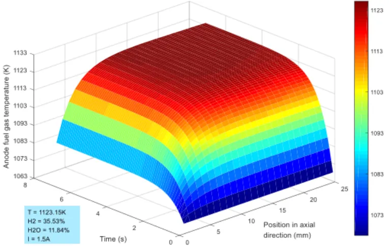
In order to verify the multi-dimensional real-time fuel cell thermal dynamic performance, the temperature of the fuel gas in the anode tube channel is also simulated. The test is conducted under furnace temperature of 1123.15K, and a fuel gas composition of 35.53% H2 and 11.84% H2O. 25 CV configuration has been used in the simulation. As can be seen from Fig. 16, the temperature of the fuel gas in the anode tube can reach its steady-state in about 3s, after a 1.5A current step input. The input fuel gas temperature is 1073.15K, and it reaches its highest temperature near the outlet part of the tube
channel by 1123.15K, since it is heated by the fuel cell solid phase along the channel gradually.
Fig. 16. Real-time SOFC anode gas temperature distributions
VI. CONCLUSIONS
This paper proposed a multi-dimensional, multi-physical SOFC model for real-time applications. The numerical stiffness in the built model was analyzed and proofed to have a large perturbation range. A parallel two-stage third-order ODE solver is proposed for the strong stiff SOFC model real-time simulation.
The multi-dimensional real-time fuel cell model couples thermal, electrochemical and fluidic domains, and the existence of ODEs numerical stiffness lead to the commonly used ODE algorithms fail to acquire satisfying performance. For overcoming the SOFC model stiffness variation in the real-time simulation, the proposed real-time extended Rosenbrock method is proofed to be A-stable with strong stiff robustness, and suitable for the SOFC model. The programming language coded solver can be easily implemented to any real-time applications without platform dependency.
Simulation result shows that the stability can be maintained in strong stiff conditions. The experimental results indicate the developed real-time SOFC model with over hundreds control volumes configuration is capable to be executed in a 3.4 GHz processor in millisecond level. The real-time SOFC simulation results correspond very well with the experimental ones. The proposed multi-dimensional, multi-physical SOFC model with the proposed solver is therefore satisfied the real-time simulation requirement and can be applied to online control and diagnosis applications.
REFERENCES
[1] S. Kang, K. Ahn, “Dynamic modeling of solid oxide fuel cell and engine hybrid system for distributed power generation,” Applied Energy, vol. 195, pp. 1086-1099, Jun. 2017.
[2] T. Lan, K. Strunz, “Multi-physics transients modeling of solid oxide fuel cells: methodology of circuit equivalents and use in EMTP-type power system simulation,” Trans. Energy Convers., vol. 32, no. 4, pp. 1309-1321, Apr. 2017.
[3] X. J. Luo, K. F. Fong, “Development of a 2D dynamic model for hydrogen-fed and methane-fed solid oxide fuel cells,” J. Power Sources, vol. 328, pp. 91-104, Oct. 2016.
[4] A. Bertei, E. Ruiz-Trejo, F. Tariq, V. Yufit, A. Atkinson, N.P. Brandon, “Validation of a physically-based solid oxide fuel cell anode model combining 3D tomography and impedance spectroscopy,” Intern. J. Hydrogen Energy, vol. 41, no. 47, pp. 22381-22393, Dec. 2016
[5] S. Shen, M. Ni, “2D segment model for a solid oxide fuel cell with a mixed ionic and electronic conductor as electrolyte,” Intern. J. Hydrogen Energy, vol. 40, no. 15, pp. 5160-5168, Apr. 2015
[6] Y. Huangfu, F. Gao, A. Abbas-Turki, et al., “Transient dynamic and modeling parameter sensitivity analysis of 1D solid oxide fuel cell model,” Energy Conver. Managem., vol. 71. pp. 172-185, Mar. 2013. [7] Sergio Yesid Gómez, Dachamir Hotza, “Current developments in
reversible solid oxide fuel cells,” Renewable and Sustainable Energy Reviews, vol. 61, pp. 155-174, Aug. 2016.
[8] R.T. Nishida, S.B. Beale, J.G. Pharoah, “Comprehensive computational fluid dynamics model of solid oxide fuel cell stacks,” Intern. J. Hydrogen Energy, vol. 41, no. 45, pp. 20592-20605, Dec. 2016
[9] B. J. Spivey, T. F. Edgar, “Dynamic modeling, simulation, and MIMO predictive control of a tubular solid oxide fuel cell,” Journal of Process Control, vol. 22, no. 8, pp: 1502-1520. Sep. 2012.
[10] V. Menon, V. M. Janardhanan, S. Tischer, Olaf Deutschmann, “A novel approach to model the transient behavior of solid-oxide fuel cell stacks,” Journal of Power Sources, vol. 214, pp. 227-238, Sep. 2012.
[11] X. Jin, X. Xue, “Mathematical modeling analysis of regenerative solid oxide fuel cells in switching mode conditions,” Journal of Power Sources, vol. 195, no.19 pp.6652-6658, Oct. 2010.
[12] C. Restrepo, T. Konjedic, C. Guarnizo et al., “Simplified Mathematical Model for Calculating the Oxygen Excess Ratio of a PEM Fuel Cell System in Real-Time Applications,” IEEE Transactions on Industrial Electronics, vol. 61, no. 6, pp. 2816-2825, June 2014.
[13] Y. X. Wang and Y. B. Kim, “Real-Time Control for Air Excess Ratio of a PEM Fuel Cell System,” IEEE/ASME Transactions on Mechatronics, vol. 19, no. 3, pp. 852-861, June 2014.
[14] N. Katayama and S. Kogoshi, “Real-Time Electrochemical Impedance Diagnosis for Fuel Cells Using a DC-DC Converter,” IEEE Transactions on Energy Conversion, vol. 30, no. 2, pp. 707-713, June 2015.
[15] Y. Lee, J. Kim, S. Yoo, “On-line and real-time diagnosis method for proton membrane fuel cell (PEMFC) stack by the superposition principle,” J. Power Sources, vol. 326, pp. 264-269, Sep. 2016. [16] V. Zaccaria, D. Tucker, A. Traverso, “A distributed real-time model of
degradation in a solid oxide fuel cell, part I: Model characterization,” Journal of Power Sources, vol. 311, pp. 175-181, Apr. 2016.
[17] C. Wu, J. Chen, C. Xu and Z. Liu, “Real-Time Adaptive Control of a Fuel Cell/Battery Hybrid Power System with Guaranteed Stability,” IEEE Trans. Control Sys. Tech., vol. 25, no. 4, pp. 1394-1405, July 2017. [18] T. Fletcher, R. Thring, M. Watkinson, “An Energy Management Strategy
to concurrently optimize fuel consumption & PEM fuel cell lifetime in a hybrid vehicle,” International Journal of Hydrogen Energy, vol. 41, no. 46, pp. 21503-21515, Dec. 2016.
[19] F. Gao, B. Blunier, M. Simoes, and A. Miraoui, “PEM Fuel Cell stack modeling for real-time emulation in hardware-in-the-loop applications,” IEEE Trans. Energy Convers., vol. 26, no. 1, pp. 184–194, Mar. 2011. [20] P. Massonnat, F. Gao, R. Roche, D. Paire, et al., “Multiphysical,
multidimensional real-time PEM fuel cell modeling for embedded applications,” Energy Conv. Manag., vol. 88, pp. 554-564, Dec. 2014. [21] C. A. R. Paja, A. Romero and R. Giral, “Evaluation of Fixed-Step
Differential Equations Solution Methods for Fuel Cell Real-Time Simulation,” Intern. Conf. Clean Electrical Power, Capri, 2007. [22] E. Breaz, F. Gao, D. Paire and R. Tirnovan, “Fuel cell modeling With
dSPACE and OPAL-RT real time platforms,” IEEE Transportation Electrification Con. and Expo (ITEC), Dearborn, MI, 2014, pp. 1-6. [23] J. H. Jung, S. Ahmed and P. Enjeti, “PEM Fuel Cell Stack Model
Development for Real-Time Simulation Applications,” IEEE Trans. Industrial Electronics, vol. 58, no. 9, pp. 4217-4231, Sept. 2011. [24] R. Ma, F. Gao, E. Breaz, Y. Huangfu, P. Briois, “Multi-Dimensional
Reversible Solid Oxide Fuel Cell Modeling for Embedded Applications,” IEEE Trans. Energy Convers., vol. PP, no. 99, pp. 1-1.
[25] C. Xuenian, L. Dequi and L. Shouju, “A class of parallel algorithms of real-time numerical simulation for stiff dynamic system,” J. of Systems Engineering and Electronics, vol. 11, no. 4, pp. 51-58, Dec. 2000. [26] H. H. Rosenbrock, “Some general implicit processes for the numerical
solution of differential equations,” The Computer Journal, vol. 5, no. 4, pp. 329-330, Jan. 1963.
[27] Q. Feng et al., “Improved biogeography-based optimization with random ring topology and Powell's method,” Applied Mathematical Modelling, vol. 41, pp. 630-649. Jan. 2017.
[28] P. Parks, “Liapunov and the Schur-Cohn stability criterion,” IEEE Transactions on Automatic Control, vol. 9, no. 1, pp. 121-121, Jan 1964.