Technical report: supervised training of convolutional spiking neural networks with PyTorch

HAL Id: hal-02870276

https://hal.archives-ouvertes.fr/hal-02870276

HAL is a multi-disciplinary open access archive for the deposit and dissemination of sci-entific research documents, whether they are

pub-L’archive ouverte pluridisciplinaire HAL, est destinée au dépôt et à la diffusion de documents scientifiques de niveau recherche, publiés ou non,

Technical report: supervised training of convolutional

spiking neural networks with PyTorch

Romain Zimmer, Thomas Pellegrini, Srisht Fateh Singh, Timothée Masquelier

To cite this version:

Romain Zimmer, Thomas Pellegrini, Srisht Fateh Singh, Timothée Masquelier. Technical report: su-pervised training of convolutional spiking neural networks with PyTorch. [Technical Report] CERCO UMR 5549, CNRS – Université Toulouse 3, Toulouse, France. 2019. �hal-02870276�

Technical report: supervised training of

convolutional spiking neural networks with

PyTorch

Romain Zimmer1, 2, Thomas Pellegrini2, Srisht Fateh Singh1, and Timothée Masquelier1

1_{CERCO UMR 5549, CNRS – Université Toulouse 3, Toulouse, France} 2_{IRIT, Université de Toulouse, Toulouse, France}

Recently, it has been shown that spiking neural networks (SNNs) can be trained efficiently, in a supervised manner, using backpropagation through time. In-deed, the most commonly used spiking neuron model, the leaky integrate-and-fire neuron, obeys a differential equation which can be approximated using dis-crete time steps, leading to a recurrent relation for the potential. The firing thresh-old causes optimization issues, but they can be overcome using a surrogate gra-dient. Here, we extend previous approaches in two ways. Firstly, we show that the approach can be used to train convolutional layers. Convolutions can be done in space, time (which simulates conduction delays), or both. Secondly, we include fast horizontal connections à la Denève: when a neuron N fires, we subtract to the potentials of all the neurons with the same receptive the dot product between their weight vectors and the one of neuron N. As Denève et al. showed, this is useful to represent a dynamic multidimensional analog signal in a population of spiking neurons. Here we demonstrate that, in addition, such connections also allow implementing a multidimensional send-on-delta coding scheme. We vali-date our approach on one speech classification benchmarks: the Google speech command dataset. We managed to reach nearly state-of-the-art accuracy (94%) while maintaining low firing rates (about 5Hz). Our code is based on PyTorch and is available in open source athttp://github.com/romainzimmer/s2net.

C

1. Introduction 3

2. Literature review 3

3. Integrate and Fire neuron models 6

3.1. Leaky Integrate and Fire (LIF) . . . 6

3.2. Non-Leaky Integrate and Fire (NLIF) . . . 6

3.3. Input current . . . 6

4. Spiking neural networks and event-based sampling 7 4.1. Rate vs Temporal Coding . . . 7

4.2. Send-on-Delta . . . 7

4.3. Send-on-Delta with Integrate and Fire neurons . . . 7

4.4. multi-dimensional send-on-delta . . . 9

5. Deep Spiking Neural Networks 11 5.1. LIF neurons as Recurrent Neural Networks cells . . . 11

5.2. Surrogate gradient . . . 11

5.3. Feed-forward model . . . 12

5.3.1. Fully-connected spiking layer . . . 12

5.3.2. Convolutional spiking layer . . . 13

5.3.3. Readout layer . . . 13

5.4. Recurrent Model . . . 13

5.5. Penalizing the number of spikes . . . 13

6. Experiments 15 6.1. Speech Commands dataset . . . 15

6.1.1. Preprocessing . . . 15

6.1.2. Architecture . . . 15

6.1.3. Training and evaluation . . . 17

6.1.4. Results . . . 17

7. Discussion 19 A. Appendix 20 A.1. Discrete time approximation . . . 20

1. I

Current Artificial Neural Networks (ANN) come from computational models of biological

neurons like McCulloch-Pitts Neurons [McCulloch and Pitts, 1943] or the Perceptron [Rosenblatt, 1958]. Yet, they are characterized by a single, static, continuous-valued activation. On the contrary,

biological neurons use discrete spikes to compute and transmit information, and spike tim-ing, in addition to the spike rates, matters. SNNs are, thus, more biologically realistic than ANNs. Their study might help understanding how the brain encodes and processes informa-tion, and lead to new machine learning algorithms.

SNNs are also hardware friendly and energy efficient if implemented on specialized neu-romorphic hardware. These neuneu-romorphic, non von Neumann architectures are highly con-nected and parallel, require low-power, and collocate memory and processing. Thus, they do not suffer from the so-called "von Neumann bottleneck" due to low bandwith between CPU and memory [Backus, 1978]. Neuromorphic architectures have also received increased at-tention due to the approaching end of Moore’s law. Neuromorphic computers might enable faster, more power-efficient complex calculations and on a smaller footprint than traditional von Neumann architectures. (See [Schuman et al., 2017] for a survey on neuromorphic com-puting and neural networks in hardware).

Neuroscientists have proposed many different, more or less complex, models to describe the dynamics of spiking neurons. The Hodgkin-Huxley neuron [HODGKIN and HUXLEY, 1952] models ionic mechanisms underlying the initiation and propagation of action potentials. More phenomenological models such as the leaky integrate-and-fire model with several vari-ants e.g. the quadratic integrate and fire model, adaptive integrate and fire, and the expo-nential integrate-and-fire model have proven to be very good at predicting spike trains de-spite their apparent simplicity [Jolivet et al., 2005]. Other models such as Izhikevich’s neuron model [Izhikevich, 2003] try to combine the biological plausibility of Hodgkin-Huxley-type dynamics and the computational efficiency of integrate-and-fire neurons. See [Burkitt, 2006] for a review of the integrate and fire neuron models.

However, these models have been designed to fit experimental data and cannot be directly used to solve real life problems.

2. L

Various models of spiking neural networks for machine learning have alreay been proposed. Recurrent Spiking Neural Networks (RSNNs) have been trained to generate dynamic pat-terns or to classify sequential data. They can have one or more populations of neurons with random or trainable connections. The computational power of recurrent spiking neural net-works has been theoretically proven in [Maass and Markram, 2004] and models such as liquid state machines [Maass et al., 2002] and Long short-term memory Spiking Neural Networks (LSNNs) [Bellec et al., 2018] have been proposed.

de-rives a method to convert continuous-valued deep networks to spiking neural networks for image classification. However, these models only use rate coding.

Spiking neural networks can also be trained directly using spike-timing-dependent plas-ticity (STDP), a local rule based on relative spike timing between neurons. This is an un-supervised training rule to extract features that can be used by an external classifier. For instance, [Kheradpisheh et al., 2018] have built a convolutional SNN trained with STDP and used a Support Vector Machine (SVM) for classification. More recently, [Mozafari et al., 2018, Mozafari et al., 2019] proposed a reward modulated version of the STDP to train a classifi-cation layer on top of the STDP network and thus, does not require any external classifier. These networks usually use latency coding with at most one spike per neuron. The label predicted by the network is given by the first spike emitted in the output layer. Backprop-agation has also been adapted to this sort of coding, by computing gradients with respect to latencies [Mostafa, 2017, Comsa et al., 2019, Kheradpisheh and Masquelier, 2019]. The “at most one spike per neuron” limit is not an issue with static stimuli (e.g. images), yet it is not suitable for dynamic stimuli like sounds or videos.

Backpropagation through time (BPTT) [Mozer, 1995] cannot be used directly to train spik-ing neural network because of their binary activation function (see 5.2). The same problem occurs for quantized neural networks [Hubara et al., 2016]. However, the gradient of these functions can be approximated. For instance, [Bengio et al., 2013] studies various gradient estimators (e.g. straight-through estimator) for stochastic neurons and neurons with hard activation functions. Binarized networks with with performances similar to standard neural networks have been developed [Courbariaux and Bengio, 2016]. They use binary weights and activations, whereas only activations are binary in this project. Yet, their encoding cannot be sparse as they use {-1, 1} as binary values.

These ideas can also be used to train spiking neural networks. [Neftci et al., 2019] gives an overview of existing approaches and provides an introduction to surrogate gradient methods, initially proposed in ref. [Bohte et al., 2000, Esser et al., 2016, Wu et al., 2018, Bellec et al., 2018, Shrestha and Orchard, 2018, Zenke and Ganguli, 2018]. Moreover, [Kaiser et al., 2018] proposes a Deep Continuous Local Learning (DECOLLE) capable of learning deep spatio-temporal representations from spikes by approximating gradient backpropagation using locally syn-thesized gradients. Thus, it can be formulated as a local synaptic plasticity rules. However, it requires a loss for each layer and these losses have to be chosen arbitrarily. Another approach has been proposed by [Huh and Sejnowski, 2018]: they replaced the threshold by a gate func-tion with narrow support, leading to a differentiable model which does not require gradient approximations.

The encoding method used in this project to represent signals with spikes (See Spiking neu-ral networks and event-based sampling) is very similar to the matching pursuit algorithm proposed by S. Mallat [Mallat and Zhifeng Zhang, 1993]. This algorithm adaptively decom-poses a signal into a linear expansion of waveforms that are selected from a redundant dic-tionary of functions. Starting with the raw signal, waveforms are greedily chosen one at a time in order to maximally reduce the approximation error. At each iteration, the projection of the signal on the selected waveform is removed. The algorithm stops when the energy of

the remaining signal is small enough. [Bourdoukan et al., 2012] used a similar idea to rep-resent efficiently a signal with the activity of a set of neurons. The potential of each neuron depends on the projection of the signal on the direction of the neuron. And each neuron compete to reconstruct the signal. However, for this project, the goal is to classify an input signal and not to reconstruct it. Thus, the goal is to find the most interesting direction for classification and not the ones that best reconstruct the signal. The link between send-on-delta and integrate-and-fire event-based sampling schemes has already been highlighted by [Moser and Lunglmayr, 2019]. And [Moser, 2016] proposes a mathematical metric analysis of integrate-and-fire sampling. However, they use negative spikes if the "potential" goes under the opposite of the threshold and only consider 1 dimensional input signals.

3. I

F

3.1. LEAKYINTEGRATE ANDFIRE(LIF)

In the standard Leaky Integrate and Fire (LIF) model, the sub-threshold dynamics of the membrane of the it hneuron is described by the differential equation [Neftci et al., 2019]

τmem

dUi

d t = −(Ui−Urest) + R Ii (3.1)

where Ui(t ) is the membrane potential at time t , Ur est is the resting membrane potential,

τmemis the membrane time constant, Ii is the current injected into the neuron and R is the resistance. When Uiexceeds a threshold Bi, the neuron fires and Uiis decreased. The −(Ui−

Urest) term is the leak term that drives the potential towards Urest.

3.2. NON-LEAKYINTEGRATE ANDFIRE(NLIF)

If there is no leak, the model is called Non-Leaky Integrate and Fire (NLIF) and the corre-sponding differential equation is

τmem

dUi

d t = R Ii (3.2)

Without loss of generality, we will take R = 1 and Ur est = 0 in the following.

3.3. INPUT CURRENT

The input current can be defined as the projection of the input spikes along the preferred direction of neuron i given by Wi, the it hrow of W.

Ii= X j Wi jSin_j (3.3) where Sj(t ) =Pkδ(t − t j

k) if neuron j fires at time t = t j

1, t

j

2, ....

Or, it can be a be governed by another differential equation, e.g. a leaky integration of these projections τsyn d Ii d t = −Ii+ X j Wi jSin_j

whereτsynis the synapse time constant.

In the former, the potential will rise instantaneously when input spikes are received whereas it will increase smoothly in the latter.

4. S

-

4.1. RATE VSTEMPORALCODING

Standard Deep Learning (DL) is based on rate coding models that only consider the firing rate of neurons. The outputs of standard DL models are thus real-valued. However, there is

evi-dence that precise spike timing can play an important role in the neural code [Gollisch and Meister, 2008], [Moiseff and Konishi, 1981], [Johansson and Birznieks, 2004]. Furthermore, computing with

sparse binary activation can require much less computing power than traditional real-valued activation. We wanted to create a model based on precise spike timing with an efficient and sparse encoding of the information. However, there is no commonly accepted theory on how real neurons encode information with spikes. Thus, we based our approach on even-based sampling theory and explained how it can be related to spiking neural networks.

4.2. SEND-ON-DELTA

Most of the time, the input signal is real-valued and has to be encoded as spike trains. This can be done using an event-based sampling strategy. In this work, the Send-On-Delta (SoD) sampling strategy [Miskowicz, 2006] is used.

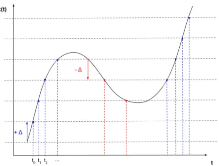
The SoD strategy is a threshold-based sampling strategy. The sampling is triggered when a significant change is detected in signal x, i.e. the :

tk= inft ≥tk−1{t , |x(t) − x(tk−1)| ≥ ∆} (4.1)

where tk is the time of the kt h sampling event. Changes in the signal can be either an increase or a decrease (See Fig. 4.1).

This strategy is used by event-based cameras and is very efficient to remove temporal re-dundancy as sampling will only occur if the input signal changes.

4.3. SEND-ON-DELTA WITHINTEGRATE ANDFIRE NEURONS

This encoding scheme can be achieved by two NLIF neurons with lateral connections and whose input is the derivative of the signal.

Let,

I (t ) = w ˙x(t) and U (tk+) = 0

with t_k+(resp. t_k−) the time just after (resp. before) the kt h spike has been emitted and w a scaling factor.

Then, for the IF model we have,

Figure 4.1: Send-on-delta sampling strategy. Blue dots represent sampling due to a signifi-cant increase, red dots represent sampling due to a signifisignifi-cant decrease.

If the threshold is B = w2, the next spike is emitted at t_k+1+ such that

t_k+1= inft ≥tk{t , U (t ) ≥ w

2_}

= inft ≥tk{t , sign(w )(x(t ) − x(tk)) ≥ |w|}

Depending on the sign of w , the neuron will detect an increase or a decrease of at least |w| in the signal since the last emitted spike, provided that the potential is reset when a spike is emitted, i.e. Ui(t_k+) = 0 for all k.

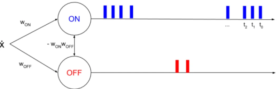
To achieve a send-on-delta sampling, two IF neurons are needed. One "ON" neuron with

wON> 0 and one "OFF" neuron with wOFF< 0, and their potentials have to be reset when any

of them fires. Indeed, the reference value of the signal must be updated when sampling oc-curs. This can be done by adding lateral connections between the "ON" and "OFF" neurons. Let tk be the kt htime that any of the "ON" and "OFF" neurons fires. And suppose that the "ON" neuron fires at time t_k+1. We have

UON(t_k+1− ) = wON(x(tk+1) − x(tk)) = w_ON2 (4.2) =⇒ UOFF(t_k+1− ) = wOFF(x(tk+1) − x(tk)) = wOFFwON (4.3)

Applying the same reasoning for a spike emitted by the "OFF" neuron, we find that the weight of the lateral connection between the "ON" and the "OFF" neurons must be −wOFFwON

Figure 4.2: Architecture for SoD encoding with two IF neurons and spike train generated for the example presented in figure 4.1

Note that, the reset is equivalent to an update of the input signal for each neuron. For example, if the "ON" neuron fires at time t_k+1

UON(t_k+1− ) − wON2 = wON(x(tk+1) − x(tk) − wON)

UOFF(t_k+1− ) − wOFFwON= wOFF(x(tk+1) − x(tk) − wON)

If an increase of at least wONis detected, then the reference signal is increased by wONfor

each neuron.

In this case, the deltas for the detection of an increase or a decrease are different. To have the same delta, wOFFshould be equal to −wON.

4.4. MULTI-DIMENSIONAL SEND-ON-DELTA

The previous results only apply to 1-dimensional signal. For a m-dimensional signal, each di-mension can be tracked independently. The number of neurons required is thus 2*m. How-ever, tracking each dimension independently is not efficient if the coordinates of the signal are correlated. Thus, we propose a multi-dimensional generalization of send-on-delta and the corresponding network architecture, inspired by [Bourdoukan et al., 2012].

Instead of detecting changes in each dimension separately, we can detect changes in the projection of the signal along a given sampling direction. In this case, rather than simply increasing or decreasing the reference value of the signal when sampling occurs, it has now to be moved in the sampling direction (see Fig. 4.3).

Let us consider a population of n neurons. Each neuron i ∈ [[0,n−1]] has its own "preferred" direction wi.

After the kt hspike emitted by any of these neurons, we have for for neuron i

Figure 4.3: Left: independent tracking of each dimension, Right: tracking along a given direc-tion

The threshold of the it h neuron is set to kwik2and the weight of lateral connections be-tween neurons i and j to − < wj, wi>. Just after the reset, we have

Uj(t_k+1+ ) =< wj, x(tk+1) − x(tk) − wi>

Thus, if neuron i fires, wiis added to the signal reference value of all neurons.

Note that, if wiand wj are orthogonal the weight of lateral connections is 0 and neurons i and j are independent. If wj and wi are collinear, then the potential is reset to exactly 0. In particular, this is the case for neuron i .

Interestingly, the multi-dimensional generalization of SoD yields the same networks ar-chitecture as in [Bourdoukan et al., 2012] for optimal spike-based representations. The only difference is that in [Bourdoukan et al., 2012], the threshold is set tokwik2

2 instead of kwik2as

they want to minimize the distance between the signal and the samples. It can be interpreted very easily in the context of event-based sampling. If sampling is associated with an update of the reference signal of ±∆, then sampling reduces the reconstruction error as soon as the signal deviates by more than ∆₂ from the reference.

LIF neurons can be used as well with the same architecture. The sampling scheme would be equivalent to SoD with leak. Depending on the leak, only abrupt changes would be detected.

5. D

S

N

N

Based on [Neftci et al., 2019] and the results of section 4, we implemented a spiking neural network in PyTorch. Spiking Layers can be Fully-Connected or Convolutional and with or without lateral connections. The neural network can be a standard feed forward network or a pool of neurons with recurrent connections.

A PyTorch based implementation of the different layers is available at http://github. com/romainzimmer/s2net.

5.1. LIFNEURONS ASRECURRENTNEURALNETWORKS CELLS

The differential equations of LIF models can be approximated by linear recurrent equations in discrete time (See Appendix A.1). Introducing the reset term Ri[n] corresponding to lateral connections, the neuron dynamics can now be fully described by the following equations.

Ui[n] = β(Ui[n − 1] − Ri[n]) + (1 − β)Ii[n] (5.1) Ii[n] = X j Wi jSin_j [n] (5.2) Ri[n] = (W · WT· Sout[n])i (5.3) Sout_i [n] = Θ(Ui[n] − Bi) (5.4) Bi= kWik2 (5.5) whereβ = exp(−_τ∆t

mem) andΘ is the Heaviside step function.

Thus, LIF neurons can be modeled as a Recurrent Neural Network (RNN) cells whose state and output at time step n are given by (U [n], I [n]) and S[n] respectively [Neftci et al., 2019].

In practice, we used a trainable threshold parameter bifor neuron i , such that

Si[n] = Θ( Ui[n] Bi+ ²− bi) = Θ( Ui[n] kWik2+ ²− bi )

with bi initialized to 1 and² = 10−8. We normalize with kWik2as the scale of the surrogate gradient is fixed.

5.2. SURROGATE GRADIENT

The RNN model can be implemented with traditional Deep Learning tools. However, one major issue has to be addressed regarding the threshold activation function.

The derivative of the Heaviside step function is 0 everywhere and is not defined in 0. Thus, no gradient can be back-propagated through it. To solve this problem, [Neftci et al., 2019] propose to approximate the derivative of the Heaviside step function.

Figure 5.1: Approximation of the derivative of the Heaviside step function

For instance, one can approximate the Heaviside step function by a sigmoid function with a scale parameterσ ≥ 0 controlling the quality of the approximation.

Thus,

Θ0_{≈ sig}0

σ (5.6)

whereσ ∈ R+and sig_σ: x →_1+e1−σx

5.3. FEED-FORWARD MODEL

We designed a feed-forward model composed of multiple spiking layers and a readout layer. The input of a spiking layer is a spike train except for the first layer whose input is a multi-dimensional real-valued signal . Each layer outputs a spike train except for the readout layer that outputs real values that can be seen as a linear combination of spikes.

5.3.1. FULLY-CONNECTED SPIKING LAYER

For the fully-connected spiking layer, the input current at each time step is a weighted sum of the input spikes emitted by the previous layer at the given moment (or a weighted sum of the input signal if it is the first layer). The state and the output of the cells are updated following the above equations.

5.3.2. CONVOLUTIONAL SPIKING LAYER

For the convolutional spiking layer, the input current at each time step is given by a 1D (0D + time),2D (1D + time) or 3D (2D + time) convolution between a kernel and the input spike train. Note that convolution in time can be seen as propagation delays of the input spikes.

In this layer, lateral connections are only applied between neurons that have the same re-ceptive field, i.e. locally between the different channels. For the it h receptive field at time step n, when lateral connections are used, the reset term for channel p is

Ri ,p[n] = X

l

< ˜Wk, ˜Wl> Si ,l[n − 1]

Where ˜Wpis the vectorized form of Wp, the kernel corresponding to the pt h channel and the sum is over the different channels.

5.3.3. READOUT LAYER

For the readout layer, [Neftci et al., 2019] proposed to use non-firing neurons. Thus, there is no reset nor lateral connections in this layer. For classification tasks, the dimension of the output is equal to the number of labels and the label probabilities are given by the softmax of the maximum value over time of the membrane potential of each neuron.

In practice, we have found that using time-distributed fully connected layer and taking the mean activation of this layer over time as output makes training more stable, at least with the datasets we have used. Thus, the output is the mean over time of a linear combination of input spikes.

5.4. RECURRENTMODEL

In the recurrent model, a pool of neurons with recurrent connections (output is fed back to the neurons) is used instead of stacking multiple layers. The input current for this model can also be computed using convolutions. And in this case, recurrent connections are only applied locally, i.e. between the channels for a given receptive field.

5.5. PENALIZING THE NUMBER OF SPIKES

A simple way to penalize the number of spikes is to apply a L1 or L2 loss on the total number of spikes emitted by each layer.

However, due to the surrogate gradient, some neurons will be penalized even if they haven’t emitted any spike.

#spikes = 1 K N X n X k Sk[n] = 1 K N X n X k S2_k[n]

where K is the number of neurons and N is the number of time steps.

Replacing Sk[n] by Sk[n]2is a simple way to ensure that the regularization will not be ap-plied to neurons that have not emitted any spikes, i.e. for which Sk[n] = 0.

Indeed,

d S_k2[n]

dUk[n]= 2 ∗ S

k[n] ∗ si g_σ0(Uk[n]) which is 0 when Sk[n] = 0.

6. E

During this project, we mainly worked with feed-forward convolutional models on the Speech Commands dataset [Warden, 2018] as the goal was to compare spiking neural networks to standard deep learning models.

6.1. SPEECHCOMMANDS DATASET

The Speech Commands dataset is a dataset of short audio recordings (at most 1 second, sam-pled at 16 kHz) of 30 different commands pronounced by different speakers for its first ver-sion and 35 for the second. All experiments were conducted on the first verver-sion of the dataset.

The task considered is to discriminate among 12 classes:

• 10 commands: "yes", "no", "up", "down", "left", "right", "on", "off", "stop", "go" • unknown

• silence

The model is trained on the whole dataset. Commands that are not in the classes are la-belled as unknown and silence training data are extracted from the background noise files provided with the dataset. See Table 6.1.

Authors of [Warden, 2018] also provide validation and testing datasets that can be directly used to evaluate the performance of a model.

6.1.1. PREPROCESSING

Log Mel filters together with their derivatives and second derivatives are extracted from raw signals using the python package LibROSA [McFee et al., 2015]. For the FFT, we used a win-dow size of 30 ms and a hop length of 10 ms, which also corresponds to the time step of the simulationδt. These are typical values in speech processing. Then, the log of 40 Mel filter co-efficients were extracted using a Mel scale between 20 Hz and 4000 Hz only as this frequency band contains most of speech signal information (see Fig 6.1).

Finally, the spectrograms corresponding to each derivative order are re-scaled to ensure that the signal in each frequency has a variance of 1 across time and are considered as 3 different input channels.

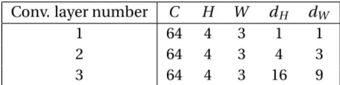
6.1.2. ARCHITECTURE

For this task, we used 3 convolutional spiking layers with the same lateral connections as in the multi-dimensional send-on-delta architecture. The readout layer is a time distributed fully connected readout layer. Each convolutional layer has aβ trainable parameter control-ling the time constant of the layer, C channels and one threshold parameter b per channel.

convolu-Words (V1 and V2) Number of Utterances Bed 2,014 Bird 2,064 Cat 2,031 Dog 2,128 Down 3,917 Eight 3,787 Five 4,052 Four 3,728 Go 3,880 Happy 2,054 House 2,113 Left 3,801 Marvin 2,100 Nine 3,934 No 3,941 Off 3,745 On 3,845 One 3,890 Right 3,778 Seven 3,998 Sheila 2,022 Six 3,860 Stop 3,872 Three 3,727 Tree 1,759 Two 3,880 Up 3,723 Wow 2,123 Yes 4,044 Zero 4,052

Words (V2 only) Number of Utterances Backward 1,664

Forward 1,557 Follow 1,579

Learn 1,575

Visual 1,592

Table 6.1: Number of recordings in the speech commands dataset (extracted from [Warden, 2018]).

tional layers have a stride of 1 and dilation factors of dHand dWalong "time" and "frequency" axes respectively. See Table 6.2 for details.

The scale of the surrogate gradient was set to 10.

Conv. layer number C H W dH dW

1 64 4 3 1 1

2 64 4 3 4 3

3 64 4 3 16 9

Table 6.2: Parameters of each convolutional layer for the speech commands dataset

6.1.3. TRAINING AND EVALUATION

The model was trained using the Rectified-Adam optimizer [Liu et al., 2019] with a learning rate of 10−3, for 30 epochs with 1 epoch of warm-up, a weight decay of 10−5. For each layer

l = 1,...,L, a regularization loss Lr(l ) was added with a coefficient 0.1 ∗_Ll to enforce sparse

activity. Lr(l ) = 1 2K N X n X k S2_k[n]

Gradient values were clipped to [−5,5], β to [0,1] and b to [0,+∞[

6.1.4. RESULTS

This network achieves 94% accuracy on this task with a mean firing rate of roughly 5Hz. Thus, the activation of the network is very sparse. Moreover, the trade-off between sparsity and performance can be controlled by the regularization coefficient (see Fig. 6.2).

In comparison, standard deep learning models achieve an accuracy of 96-97% [de Andrade et al., 2018]. These experimental results were obtained using lateral connections. However, we managed

to get similar performances without them. Thus, we would like to further explore the impact of these connections for other tasks. Furthermore, we have found that recurrence through time is not necessarily useful if the discretization time step is large and processing spikes at each time step independently is enough.

Figure 6.1: Example of Mel filters extracted for the word "off".

7. D

We proposed a generalization of the send-on-delta sampling scheme to multi dimensional signal and showed that it can be achieved by a spiking neural network with lateral connec-tions. We designed a deep spiking neural network with binary sparse activation. This network can be trained using backpropagation through time with surrogate gradient methods and achieves comparable performance to standard deep learning models on the speech recogni-tion task we worked on.

These results show the potential of spiking neural networks. Although PyTorch is not par-ticularly suitable for the development of spiking neural networks, it is a very popular library in the deep learning community and we hope that this work will help to develop interest in spiking neural networks.

For future work, we would like to test our model on other tasks and especially on event data such as Dynamic Vision Sensor camera data. We would also like to continue to explore the relationships between event-based sampling theory and spiking neural networks.

A. A

A.1. DISCRETE TIME APPROXIMATION

Let’s consider the following differential equation (E) and it’s homogeneous equation (H) :

τd u

d t + u = i (E)

τd z

d t + z = 0 (H)

The solutions of (E) can be found using the variation of parameters method. The solution of (H) has the following form:

zK : t → K e−

t

τ_{= K z1(t )}

with K ∈ R

Let’s consider a solution of (E) of the form

u : t → k(t)z1(t )

Injecting this solution in E , yields the following equivalent equation

k0= i τz1 Thus, u0: t → 1 τ Z t 0 i (s)e−t −sτ _{d s}

is a particular solution of (E) and all the solutions of (E) can be written as:

uK : t → K e− t τ₊1 τ Z t 0 i (s)e−t −sτ _{d s}

Now, let’s consider t , h ∈ R.

uK(t + h) = e− h τ_{uK(t ) +}1 τ Z t +h t i (s)e−t +h−sτ _{d s}

uK(t + h) ≈ e− h τ_{uK(t ) +}i (t + h) τ Z t +h t e−t +h−sτ _{d s} = e−hτ_{uK(t ) + (1 − e}−hτ_{)i (t + h)}

In discrete time with sampling rate_h1, (E) can thus be approximated by the recurrent equa-tion:

u[n] = βu[n − 1] + (1 − β)i [n]

withβ = e−hτ_.

R

[Backus, 1978] Backus, J. (1978). Can programming be liberated from the von neumann style?: A functional style and its algebra of programs. Commun. ACM, 21(8):613–641. [Bellec et al., 2018] Bellec, G., Salaj, D., Subramoney, A., Legenstein, R. A., and Maass, W.

(2018). Long short-term memory and learning-to-learn in networks of spiking neurons.

CoRR, abs/1803.09574.

[Bengio et al., 2013] Bengio, Y., Léonard, N., and Courville, A. C. (2013). Estimating or propagating gradients through stochastic neurons for conditional computation. CoRR, abs/1308.3432.

[Bohte et al., 2000] Bohte, S. M., La Poutré, H., and Kok, J. N. (2000). Error-Backpropagation in Temporally Encoded Networks of Spiking Neurons. Neurocomputing, 48:17–37.

[Bourdoukan et al., 2012] Bourdoukan, R., Barrett, D., Deneve, S., and Machens, C. K. (2012). Learning optimal spike-based representations. In Pereira, F., Burges, C. J. C., Bottou, L., and Weinberger, K. Q., editors, Advances in Neural Information Processing Systems 25, pages 2285–2293. Curran Associates, Inc.

[Burkitt, 2006] Burkitt, A. (2006). A review of the integrate-and-fire neuron model: I. homo-geneous synaptic input. Biological cybernetics, 95:1–19.

[Comsa et al., 2019] Comsa, I.-M., Potempa, K., Versari, L., Fischbacher, T., Gesmundo, A., and Alakuijala, J. (2019). Temporal coding in spiking neural networks with alpha synaptic function. arXiv:1907.13223.

[Courbariaux and Bengio, 2016] Courbariaux, M. and Bengio, Y. (2016). Binarynet: Train-ing deep neural networks with weights and activations constrained to +1 or -1. CoRR, abs/1602.02830.

[de Andrade et al., 2018] de Andrade, D. C., Leo, S., Viana, M. L. D. S., and Bernkopf, C. (2018). A neural attention model for speech command recognition. CoRR, abs/1808.08929. [Esser et al., 2016] Esser, S. K., Merolla, P. A., Arthur, J. V., Cassidy, A. S., Appuswamy, R.,

Amir, A., Taba, B., Flickner, M. D., and Modha, D. S. (2016). Convolutional networks for fast, energy-efficient neuromorphic computing. Proceedings of the National Academy of

Sciences of the United States of America.

[Gollisch and Meister, 2008] Gollisch, T. and Meister, M. (2008). Rapid neural coding in the retina with relative spike latencies. Science, 319(5866):1108–1111.

[HODGKIN and HUXLEY, 1952] HODGKIN, A. L. and HUXLEY, A. F. (1952). A quantitative de-scription of membrane current and its application to conduction and excitation in nerve.

J. Physiol. (Lond.), 117(4):500–544.

[Hubara et al., 2016] Hubara, I., Courbariaux, M., Soudry, D., El-Yaniv, R., and Bengio, Y. (2016). Quantized neural networks: Training neural networks with low precision weights and activations. CoRR, abs/1609.07061.

[Huh and Sejnowski, 2018] Huh, D. and Sejnowski, T. J. (2018). Gradient descent for spiking neural networks. In Bengio, S., Wallach, H., Larochelle, H., Grauman, K., Cesa-Bianchi, N., and Garnett, R., editors, Advances in Neural Information Processing Systems 31, pages 1433–1443. Curran Associates, Inc.

[Izhikevich, 2003] Izhikevich, E. M. (2003). Simple model of spiking neurons. IEEE

transac-tions on neural networks / a publication of the IEEE Neural Networks Council, 14(6):1569–

1572.

[Johansson and Birznieks, 2004] Johansson, R. and Birznieks, I. (2004). First spikes in ensem-bles of human tactile afferents code complex spatial fingertip events. Nature neuroscience, 7:170–7.

[Jolivet et al., 2005] Jolivet, R., Rauch, A., and Gerstner, W. (2005). Integrate-and-fire models with adaptation are good enough: Predicting spike times under random current injection.

Advances in Neural Information Processing Systems.

[Kaiser et al., 2018] Kaiser, J., Mostafa, H., and Neftci, E. (2018). Synaptic plasticity dynamics for deep continuous local learning. CoRR, abs/1811.10766.

[Kheradpisheh et al., 2018] Kheradpisheh, S. R., Ganjtabesh, M., Thorpe, S. J., and Masque-lier, T. (2018). Stdp-based spiking deep convolutional neural networks for object recogni-tion. Neural Networks, 99:56 – 67.

[Kheradpisheh and Masquelier, 2019] Kheradpisheh, S. R. and Masquelier, T. (2019). S4NN: temporal backpropagation for spiking neural networks with one spike per neuron. arXiv. [Liu et al., 2019] Liu, L., Jiang, H., He, P., Chen, W., Liu, X., Gao, J., and Han, J. (2019). On the

variance of the adaptive learning rate and beyond. arXiv preprint arXiv:1908.03265. [Maass and Markram, 2004] Maass, W. and Markram, H. (2004). On the computational

power of circuits of spiking neurons. Journal of Computer and System Sciences, 69(4):593 – 616.

[Maass et al., 2002] Maass, W., NatschlÃd’ger, T., and Markram, H. (2002). Real-time com-puting without stable states: A new framework for neural computation based on pertur-bations.

[Mallat and Zhifeng Zhang, 1993] Mallat, S. G. and Zhifeng Zhang (1993). Matching pursuits with time-frequency dictionaries. IEEE Transactions on Signal Processing, 41(12):3397– 3415.

[McCulloch and Pitts, 1943] McCulloch, W. S. and Pitts, W. (1943). A logical calculus of the ideas immanent in nervous activity. The bulletin of mathematical biophysics, 5(4):115–133. [McFee et al., 2015] McFee, B., McVicar, M., Raffel, C., Liang, D., Nieto, O., Moore, J., Ellis, D.,

Repetto, D., Viktorin, P., Santos, J. F., and Holovaty, A. (2015). librosa: v0.4.0.

[Miskowicz, 2006] Miskowicz, M. (2006). Send-on-delta concept: An event-based data re-porting strategy. Sensors, 6.

[Moiseff and Konishi, 1981] Moiseff, A. and Konishi, M. (1981). Neuronal and behavioral sen-sitivity to binaural time differences in the owl. Journal of Neuroscience, 1(1):40–48.

[Moser, 2016] Moser, B. A. (2016). On preserving metric properties of integrate-and-fire sam-pling. In 2016 Second International Conference on Event-based Control, Communication,

and Signal Processing (EBCCSP), pages 1–7.

[Moser and Lunglmayr, 2019] Moser, B. A. and Lunglmayr, M. (2019). On quasi-isometry of threshold-based sampling. IEEE Transactions on Signal Processing, 67(14):3832–3841. [Mostafa, 2017] Mostafa, H. (2017). Supervised Learning Based on Temporal Coding in

Spik-ing Neural Networks. IEEE Transactions on Neural Networks and LearnSpik-ing Systems, pages 1–9.

[Mozafari et al., 2019] Mozafari, M., Ganjtabesh, M., Nowzari-Dalini, A., Thorpe, S. J., and Masquelier, T. (2019). Bio-inspired digit recognition using reward-modulated spike-timing-dependent plasticity in deep convolutional networks. Pattern Recognition, 94:87– 95.

[Mozafari et al., 2018] Mozafari, M., Kheradpisheh, S. R., Masquelier, T., Nowzari-Dalini, A., and Ganjtabesh, M. (2018). First-spike-based visual categorization using reward-modulated stdp. IEEE Transactions on Neural Networks and Learning Systems,

29(12):6178–6190.

[Mozer, 1995] Mozer, M. (1995). A focused backpropagation algorithm for temporal pattern recognition. Complex Systems, 3.

[Neftci et al., 2019] Neftci, E. O., Mostafa, H., and Zenke, F. (2019). Surrogate Gradient Learn-ing in SpikLearn-ing Neural Networks. arXiv e-prints.

[Rosenblatt, 1958] Rosenblatt, F. (1958). The perceptron: A probabilistic model for informa-tion storage and organizainforma-tion in the brain. Psychological Review, pages 65–386.

[Rueckauer et al., 2017] Rueckauer, B., Lungu, I.-A., Hu, Y., Pfeiffer, M., and Liu, S.-C. (2017). Conversion of continuous-valued deep networks to efficient event-driven networks for im-age classification. Frontiers in Neuroscience, 11:682.

[Schuman et al., 2017] Schuman, C. D., Potok, T. E., Patton, R. M., Birdwell, J. D., Dean, M. E., Rose, G. S., and Plank, J. S. (2017). A survey of neuromorphic computing and neural net-works in hardware. CoRR, abs/1705.06963.

[Shrestha and Orchard, 2018] Shrestha, S. B. and Orchard, G. (2018). {SLAYER}: Spike Layer Error Reassignment in Time. Neural Information Processing Systems (NIPS), (Nips). [Warden, 2018] Warden, P. (2018). Speech commands: A dataset for limited-vocabulary

speech recognition. CoRR, abs/1804.03209.

[Wu et al., 2018] Wu, Y., Deng, L., Li, G., Zhu, J., and Shi, L. (2018). Spatio-Temporal Back-propagation for Training High-Performance Spiking Neural Networks. Frontiers in

Neuro-science, 12(May):1–12.

[Zenke and Ganguli, 2018] Zenke, F. and Ganguli, S. (2018). SuperSpike: Supervised learning in multilayer spiking neural networks. Neural Computation.