HAL Id: hal-01176868
https://hal.archives-ouvertes.fr/hal-01176868
Submitted on 16 Jul 2015HAL is a multi-disciplinary open access archive for the deposit and dissemination of sci-entific research documents, whether they are pub-lished or not. The documents may come from
L’archive ouverte pluridisciplinaire HAL, est destinée au dépôt et à la diffusion de documents scientifiques de niveau recherche, publiés ou non, émanant des établissements d’enseignement et de
Practical implementation of the Corrected Force
Analysis Technique to identify the structural parameter
and load distributions
Q. Leclere, Frédéric Ablitzer, Charles Pezerat
To cite this version:
Q. Leclere, Frédéric Ablitzer, Charles Pezerat. Practical implementation of the Corrected Force Anal-ysis Technique to identify the structural parameter and load distributions. Journal of Sound and Vibration, Elsevier, 2015, 351, pp.106-118. �10.1016/j.jsv.2015.04.025�. �hal-01176868�
Practical implementation of the Corrected
Force Analysis Technique to identify the
structural parameter and load distributions
Quentin Lecl`
ere
a,∗ Fr´ed´eric Ablitzer
a,bCharles P´
ezerat
baLaboratoire Vibrations Acoustique, INSA Lyon, 25 bis avenue Jean Capelle
F-69621 Villeurbanne Cedex, FRANCE
bLUNAM Universit´e, Universit´e du Maine, CNRS UMR 6613, LAUM, Avenue
Olivier Messiaen,72085 Le Mans Cedex 9, France
Abstract
The paper aims to combine two objectives of the Force Analysis Technique (FAT): vibration source identification and material characterization from the same set of measurement. Initially, the FAT was developed for external load location and identi-fication. It consists in injecting measured vibration displacements in the discretized equation of motion. Two developments exist: FAT and CFAT (Corrected Force Anal-ysis Technique) where two finite difference schemes are used. Recently, the FAT was adapted for the identification of elastic and damping properties in a structure. The principal interests are: the identification is local and allows mapping of mate-rial characteristics, the identification can be made at all frequencies, especially in medium and high frequency domains. The paper recalls the development of FAT and CFAT on beams and plates and how it can be possible to extract material char-acteristics in areas where no external loads are applied. Experimental validations are shown on an aluminum plate with arbitrary boundary conditions, excited by a point force and where a piece of foam is glued on a sub-surface of the plate. Contact-less measurements were made using a scanning laser vibrometer. The results of FAT and CFAT are compared and discussed for material properties identifications in the regions with and without foam. The excitation force identification is finally made by using the identified material properties. CFAT gives excellent results compara-bles to a direct measurement obtained by a piezoelectric sensor. The relevance of the corrected scheme is then underlined for both source identification and material characterization from the same measurements.
Key words: source identification, Inverse problem, Material characterization, Young modulus, damping coefficient
1 Introduction
In the last decade, the Force Analysis Technique (FAT) was developed to respond to the problem of location and identification of vibration sources. The first developments were oriented for the identification of point sources, like mechanical forces or moments. In [1], the proof of concept was presented on beams with numerical and experimental validations. Close to structural intensity techniques [2,3], the basic principle of FAT consists in measuring dis-placement fields on a given meshgrid and to inject it in the equation of motion discretized by finite difference schemes. Extensions to plates [4] and shells [5,6] were made few years later. More recently, the method were adapted to more complex structures by using the Finite Element Method instead of the dis-tretized equation of motion [7,8]. Actually, The FAT has become particularly attractive, because it seems very easy to use and its generic aspect permits more complex excitations to be determined, like aeroacoustic sources [9–11] for example. Several other similar approaches can also be cited like[12–15] where the difference is in the approximation of the displacement derivatives, but the philosophy remains the same: it corresponds to a local verification of the dynamic equilibrium. The local aspect is very important since the method can be applied without any knowledge outside the studied area, like boundary conditions, other dynamic comportments or other sources. The identification of external sources by using the equation of motion is physically an inverse problem, because the goal is to determine causes (sources) from measurements of effects (displacements). Even if there is no mathematical inversion, it is in-teresting to note that the problem has the characteristic to be very sensitive to measurement uncertainties as in all inverse problems. The usual regularisation consists in filtering informations in the high wavenumber domain. In practice, several techniques were adopted, like the use of a low-pass wavenumber fil-tering [1,4,12,13], truncatures of expansions [4], Tikhonov regularisation [7,8] or the use of adapted spacings [16]. This last approach, based on a corrected finite difference scheme, is called CFAT for Corrected Force Analysis Tech-nique [17]. The CFAT has the advantage to give good results with a coarse measurement mesh, offering the possibility to regularize just by adapting the finite difference spacing as a function of the frequency.
To this point, the FAT needs only the equation of motion in the studied area. This equation contains elastic and damping material properties, so that the force identification gives good results only if their values are well known. For some materials, the properties are difficult to obtain. This is for exam-ple the case of composite materials, where elastic and damping characteristics must usually be homogenized. Since they are difficult to be assessed by model-ing, there values are experimentally obtained on test samples. The most com-mon characterization technique is the modal analysis [18], where the values of eigen frequencies and bandwidth of each mode give an idea of a global stiffness
and damping. The modal analysis presents several limitations: it can be used only in a frequency range where the structure (or the sample) has a modal comportment, the values of the material characteristics are assessed only at eigen frequencies, the characterization is global, so that the stiffness and the damping assessments contain boundaries effects and cannot distinguish any changes in the space domain. In medium and high frequency domains, or when the damping is high, the material characterization can be made from the iden-tification of the flexural wavenumber. The works of McDaniel [19], Liao [20] and later Chochol [21] show, for example, similar approaches developed on beams, where the natural wavenumber is obtained at all excitation frequen-cies by analyzing the vibration field in an area without external excitation. Fergusson et al. [22] introduced on plates the concept of correlation of the vibration field with plane waves. This work was later developed by Ichchou et al. [23] and was called Inverse Wave Correlation in Berthaut’s PhD thesis [24]. The interest of all these approaches is that the wavenumber can be assessed at all frequencies, since the structure can be excited at interest frequencies. The common principle is also the fact that the identification is realized in an area where there is no excitation, i.e. where the solutions are forced bending waves verifying the equation of motion with a null right hand side. In the same idea, an adaptation of the FAT was developed for the material charac-terization [25]. This last work shows the good assessments of material elastic and damping properties on a polymethyl methacrylate and a heterogeneous composite plates. Moreover, it shows the possibility of mapping the identified characteristics thanks to the local aspect of the FAT.
The FAT was then developed for two different objectives: source identi-fication or material characterization. The technique is practically the same; the only difference is in the unknown. In this paper, the combination of both objectives is proposed, in order to be able to identify correctly the sources exciting a structure, for which the material properties are not known (as for composite materials). In this case, only one set of measurement can be con-sidered. The paper discusses also on the practical implementation of FAT by comparing results obtained from FAT and CFAT, this last being not adapted for the material characterization until now.
The paper is organized in two major parts. The first part recalls briefly the development of FAT and CFAT on beams and plates. The adaptation of CFAT for the material properties identification is there also described. The second part presents the experimental validations obtained on a plate. This plate has unknown boundary conditions and a foam is glued on a part of its area to show the possibility to identify different elastic and damping characteristics in the space domain. The load identification is then shown using the identified properties in the equation of motion, where results of both the FAT and the CFAT are compared.
2 Theory
The FAT and CFAT have been originally developed for the identification of load distributions on beams and plates [26,17]. The FAT has been recently adapted to assess the structural parameter of plates [25]. The aim of this section is to show how the CFAT can be diverted for the same purpose. The one dimension case (beams) is treated in a first part, in order to introduce the basic concepts of the approach. The extension to two dimensions (plates) is presented in a second part.
2.1 Identification of the structural parameter for flexural beams 2.1.1 Method using standard FAT
The F AT estimation of the force distribution at a point located at x is:
pF AT(x) = EIδ∆4x− ρSω2w(x), (1) where E, I, ρ, S stand respectively for the Young’s modulus, the section mod-ulus, the density and the cross section area of the beam, and with
∂4w ∂x4 ≈ δ 4x ∆ = w(x− 2∆) − 4w(x − ∆) + 6w(x) − 4w(x + ∆) + w(x + 2∆) ∆4 , (2) where ∆ is the spacing between two consecutive points of the experimental mesh.
Let us now suppose that the force applied to the structure at x is nul. The structural parameter (EI)/(ρS) can be obtained by
EI ρS = ω2w(x) δ4x ∆ . (3)
The estimation of this structural parameter at point x thus necessitates the measurement of the beam’s vibration at 5 points around x. It is note worthy that Eq. (3) can lead to a complex value of EIρS. The elastic property can then be obtained from the real part of the structural parameter and the loss factor from the ratio between the imaginary and the real parts:
η =I ( w(x) δ4x ∆ ) /R ( w(x) δ4x ∆ ) (4)
2.1.2 Method using corrected FAT (CFAT)
The CF AT estimation of the force distribution on the beam at a point located at x is ([17]):
with µ4 = ∆ 4k4 N (2− 2 cos(kN∆))2 , (6)
and where kN is the natural wavenumber at the frequency ω:
kN4 = ρS EIω
2. (7)
If the excitation is supposed to be null at x, Eq. (5) becomes EI ρS = ω2w(x) µ4δ4x ∆ . (8)
The use of Eq. (6) into (8) leads to
EI ρS = ω 2∆4 acos 1−∆ 2 2 v u u t δ∆4x w(x) −4 (9)
As it is the case for Eq. (3), this result is potentially complex, and the corresponding loss factor can be estimated using Eq. (4).
2.2 Identification of the structural parameters for flexural plates
The possibility of identifying the structural parameter for plates using the standard FAT is the subject of a recently published paper [25]. An originality of the present work is to propose an alternative method based on CFAT, that should provide valuable results in a wider frequency range than FAT.
2.2.1 Method based on the standard FAT
The FAT estimation of the load distribution on a plate at the point coordi-nates (x, y) is ([26])
pF AT(x, y) = D(δ4x∆ + δ∆4y+ 2δ2x2y∆ )− ρhω2w(x, y), (10) where ρ, h are the plate’s density and thickness, D = Eh3(12(1−ν2))−1 ( E, ν the Young’s modulus and Poisson’s ratio), and with
δ2x2y∆ = 1 ∆4 1 ∑ p=−1 1 ∑ q=−1 ψpqw(x + p∆, y + q∆) ≈ ∂4w ∂x2∂y2, with ψ00= 4, ψ−10= ψ10 = ψ0−1 = ψ01 =−2, ψ−1−1 = ψ11 = ψ1−1 = ψ−11= 1.
Let us now suppose that the force applied to the structure at (x, y) is null. The structural parameter D/(ρh) can be assessed using
D ρh = ω2w(x, y) δ4x ∆ + δ 4y ∆ + 2δ 2x2y ∆ (11)
This estimation of D/ρh requires the measurement of the plate’s response at 13 points surrounding the estimation point. This approach to estimate the structural parameter has been originally proposed by Ablitzer et al. [25]. The next section presents an alternative approach, based on the CFAT method proposed in [26].
2.2.2 Method based on CFAT
The CFAT estimation of the load distribution on a plate at the point coor-dinates (x, y) is given by ([26]) pCF AT(x, y) = D(µ4δ∆4x+ µ4δ∆4y+ 2ν4δ2x2y∆ )− ρhω2w(x, y) (12) with µ4 = ∆ 4k4 N 4[1− cos(kN∆)]2 and ν4 = ∆ 4k4 N 8[1− cos(k√N∆ 2 ) ]2 − µ 4,
and the natural wavenumber of the plate being equal to
kN4 = ρh Dω
2. (13)
If the force is null at (x, y), then D ρh = ω2w(x, y) µ4δ4x ∆ + µ4δ 4y ∆ + 2ν4δ 2x2y ∆ . (14)
The introduction of expressions of µ and ν into Eq. (12) brings:
D ρh = ω 2 ∆4 acos 1− ∆ 2 2 v u u tδ4x∆ + δ 4y ∆ + ξ(kN∆)δ2x2y∆ w(x, y) −4 , (15) with ξ(kN∆) = (1− cos(kN∆))2 (1− cos(kN∆/ √ 2))2 − 2. (16)
This expression remains implicit because of the natural wavenumber kN that
is still in the right hand side of equation (15). However, it is possible to assess a rough value of kN using a classical FAT approach (cf. previous section), to
be used in the right hand side of equation (15). Then an updated value of kN can be assessed from the resulting value of ρhD, that can be reintroduced
in equation (15) to give a new value of kN. This iterative approach can be
conducted until convergence.
2.3 Least squares estimation of the structural parameter
Equations allowing the identification of the structural parameter are given for a single point and at a single frequency at the center of the finite differ-ence scheme, thus based on 5 or 13 measurement points for beams or plates,
respectively. It is also possible to generalize the estimation to several points, or several frequencies, using a least squares approach (cf. [25]).
For all presented estimators of the structural parameter (FAT or CFAT for beams and plates), the quantity resulting from measurements is the ratio be-tween the displacement and a finite-differences bilaplacian estimator:
A = w
B (17)
where
B = δ4x∆ for FAT and CFAT (beams) B = δ4x∆ + δ∆4y+ 2δ2x2y∆ for FAT (plates) B = δ4x∆ + δ∆4y+ ξ ( acos ( 1− ∆ 2 2√A ))
δ∆2x2y for CFAT (plates)
Note that for the latter case, the parameter A is used to correct the estima-tion of B, making Equaestima-tion (17) implicit. It can be solved using an iterative approach as explained in the previous section.
Writing Equation (17) for N measurement points at a single frequency gives a linear system of N equations and one unknown (A) that can be solved in the least squares sense :
A = (B)
H w
(B)H B (18)
where each element of the column vectors w and B represent the displacement and bilaplacian estimator at one point.The least squares estimation of A can then be used to obtained the structural parameter s (equal to EIρS for beams and ρhD for plates) :
s = ω2A for FAT (beams or plates)
s = ω2∆4 [ acos ( 1− ∆ 2 2√A )]−4
for CFAT (beams or plates)
2.4 Discussion on the joint identification of the load field and structural pa-rameter
The identification of the structural parameter has to be achieved at posi-tions where the load field is null. Moreover, FAT and CFAT are based on the local equation of motion of continuous structures, without the need to know boundary conditions. It means that every boundary condition (clamps, weld spots, stiffening ribs) will be ’seen’ as external loads, and have to be rejected for the identification of the structural parameter. If the aim of the study is to identify the load field, and if the structural parameter is not well known, it can be hazardous to determine a priori load-free areas. Of course the estimation of
the structural parameter can be done using a preliminary experiment, with a known artificial force well located. The possibility to identify jointly the load field and the structural parameter from one single measurement will be briefly discussed here.
The idea is to make a preliminary load field estimation with a generic struc-tural parameter, based on rough estimations of physical properties. Then, the structural parameter can be estimated from a subset of identification points, corresponding to low-loads areas. This low-load area is not straightforward to determine, but it can be arbitrarily defined as a fixed fraction of the total identification area (typically 1/3 or 1/2) where the preliminary rms load field estimation is minimum. Of course, this approach is suitable only if some parts of the structure are not excited, or not constraint by boundary conditions. If the load is known to be distributed on the whole structure, as it is the case for acoustic loads or turbulent boundary layers, the preliminary experiment with an artificial load cannot be avoided. Note that this preliminary exper-iment can be carried out without removing the operational load if needed: the artificial load has to be uncorrelated from the operational one (which is generally the case using a random noise generator). The response to the artifi-cial excitation only can then be obtained thanks to the Conditioned Spectral Analysis [27,28], using a standard H1 estimate referenced to the signal driving the artificial source (the response to operational loads being suppressed by the averaging process).
3 Experimental study
3.1 experimental setup
A 0.51× 0.71 m2 rectangular aluminium plate, for which the properties are
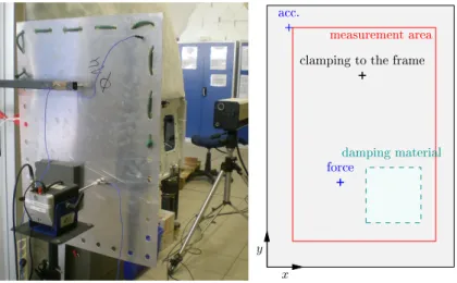
summarized in Table 1, was used in the experiments. The plate’s thickness has been calculated by measuring precisely its surface and weight. The plate had several holes along its contour. A rope has been passed through successive holes in order to attenuate flexural waves propagating near the edges. In the present experiment, about one third of the contour was equiped with such a rope (see Fig. 1). This configuration was chosen to illustrate the ability of the Force Analysis Technique to deal with arbitrary boundary conditions. Furthermore, a 15 × 15 cm2 block of adhesive damping material (foam) was added to one side of the plate to make it heterogeneous. The real part of the structural parameter of the plate with foam, given in Table 1, has been obtained just by adding a mass term (the added stiffness is assumed to be negligible). The plate was clamped to the frame at point (0.26 m, 0.52 m). The plate was excited by an electrodynamic shaker. The shaker was linked to the plate using a nylon stinger. A force sensor was mounted at the end of the stinger and glued to the plate at point (0.20 m, 0.23 m).As one aim of the experiment was to identify the excitation force, the sensitivity of the
sensor had to be known as accurately as possible. It was determined following a procedure described in appendix B.
The excitation signal was a pseudo random noise in the range [100–6400] Hz. A reference signal was provided by an accelerometer, fixed to the plate out-side the measurement area. The displacement field was measured by using a scanning laser vibrometer. Theses measurements were made in the area rep-resented in Figure 1(b) on a 28× 41 = 1148 points mesh. The dimensions of the measurement area were 0.39× 0.58 m2 and the spacing ∆ = 14.5 mm was
the same in both directions.
y x a .
measurementarea lampingtotheframe
dampingmaterial
for e
Fig. 1. Experimental setup.
Plate Young’s modulus (GPa) 69
Plate thickness h (mm) 0.965
Plate density ρ (kg/m3) 2700
Plate Poisson’s ratio 0.35
Damping material’s mass per unit area (kg/m2) 0.15 Plate mass per unit area (kg/m2) 2.6 Structural parameter without damping materialR(D/(ρh)) (m4/s2) 2.26
Structural parameter with damping material R(D/(ρh)) (m4/s2) 2.14 Table 1
Physical parameters of the studied plate
3.2 Identification of the structural parameter
In this section, the measured displacements are used to identify the struc-tural parameter D/(ρh), following the procedure described in section 2.2.
First, a point-by-point identification is carried out. For this purpose, all displacements in the frequency range [1–5] kHz are considered, which
pro-vides N = 1001 equations (one for each frequency line) for the least squares estimation of the structural parameter at each point. This identification is a preliminary step aiming at identifying areas with different mechanical proper-ties. This wide frequency approach is of course not able to estimate correctly the damping properties, that are expected to vary in the frequency domain. The results of the CFAT identification are presented in Figure 2 as a map of the real and imaginary parts of the estimated structural parameter. The CFAT estimation is realized with 10 iterations of the iterative process described in section 2.2.2, the initial value of B in equation 17 being the standard FAT re-sult. This number of iterations has been empirically found sufficient to ensure convergence. Both maps in Figure 2 make two regions clearly distinguishable. The region having the largest area corresponds to the uncovered plate. The square-shaped region of smaller area is the one where the plate is covered with damping material. The contrast between both regions is much higher on the imaginary part of the structural parameter than on its real part. The reason is that the added material provides more damping, relatively, than it increases the local mass per unit area. In addition to these two regions, very localized variations in structural parameter, both in real and imaginary parts, are observed at two locations. One location corresponds to the point where the plate is clamped and the other to the excitation point. As discussed in section 2.4, the estimation of the structural parameter is meaningless at lo-cations where either external forces or boundary condition are applied to the structure, because the identification is based on the equation of motion of the structure without external forces or links. However, such erroneous variations of the structural parameter may be easily recognized and rejected, as they are very compact compared to the load-free areas.
Fig. 2. Structural parameter estimated at each point, averaged in the frequency range [1 5] kHz. Left: real part. Right: imaginary part.
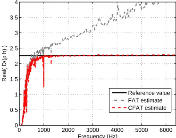
Once the spatial distribution of structural parameter has been estimated over the whole measurement area and regions with different properties were identified, the structural parameter may be estimated at all frequencies in each region. In order to illustrate the advantage of CFAT over FAT on the identifi-cation of the structural parameter, Figure 3 compares the results obtained by each procedure in the damping-free area. At low frequencies (beyond 500 Hz), FAT and CFAT give similar results. However, both procedures underestimate the actual value of the structural parameter. This is due to the fact that the spatial derivatives calculated from Eq. (2) and (11) are extremely sensitive to measurement noise when the spacing is small compared to the wavelength. The noise on the denominator of Eq (11) (for FAT) and (14) (for CFAT) is therefore much higher than the noise on the numerator, which leads to very small values of the structural parameter. At higher frequencies, the results obtained by FAT and CFAT strongly differs. Whereas the structural param-eter identified by CFAT is very close to the expected value above 1000 Hz, the one identified by FAT increasingly diverges from the actual value as the frequency increases. These results demonstrate the ability of CFAT to identify the structural parameter over a large frequency range.
0 1000 2000 3000 4000 5000 6000 0 0.5 1 1.5 2 2.5 3 3.5 4 Frequency (Hz) Real( D/( ρ h) ) Reference value FAT estimate CFAT estimate
Fig. 3. Real part of the structural parameter, least squares estimation on load-free and damping-free points. Solid black : reference value (2.4 m4/s2). Dashed blue : FAT estimation. Dashed red : CFAT estimation.
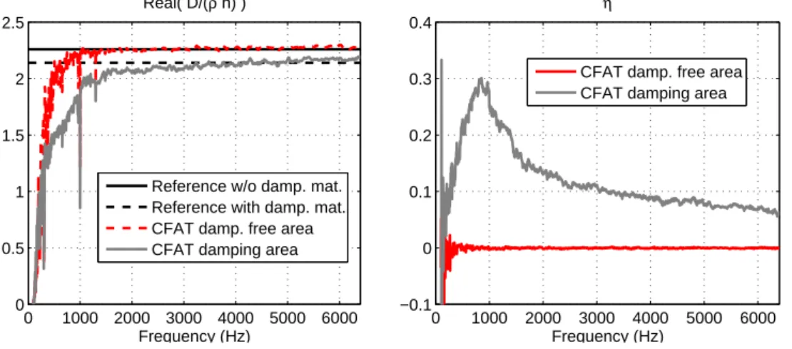
Figure 4 shows the real part and the loss factor of the structural parame-ter estimated by CFAT in the two regions previously identified (damping and damping-free areas). Regarding the real part, the curves obtained in both re-gions follow the same trend. The structural parameter is underestimated at low frequencies. The estimation becomes satisfying above 1000 Hz, though the estimation in the damping area does not match the reference value as closely as in the damping-free area. This can be explained by the fact that the damp-ing material may add stiffness to the plate, which is not taken into account in the calculation of the reference value, for which only the mass of the damping material is considered. Regarding the loss factor, the difference between the
two regions appears much more. In the damping-free area, the estimated loss factor is quasi-null. Although this result is consistent with typical values for aluminium (η ≈ 10−3), it also shows that CFAT does not allow to accurately estimate the loss factor of very lightly damped materials, because the variance of the estimation is comparable to or higher than the expected value. On the contrary, the results obtained in the damping area allows a very clear quan-tification of the loss factor, which strongly varies with frequency. The curve exhibits two different trends. Below 1000 Hz, the loss factor rapidly increases from zero to 0.3. Above 1000 Hz, it decreases quasi-exponentially. Although a non-monotonous evolution of damping with frequency is plausible for com-plex materials, only the decreasing part of the curve can be considered with confidence, since the estimation of the real part of the structural parameter is erroneous below 1000 Hz. 0 1000 2000 3000 4000 5000 6000 0 0.5 1 1.5 2 2.5 Real( D/(ρ h) ) Frequency (Hz) 0 1000 2000 3000 4000 5000 6000 −0.1 0 0.1 0.2 0.3 0.4 Frequency (Hz) η
Reference w/o damp. mat. Reference with damp. mat. CFAT damp. free area CFAT damping area
CFAT damp. free area CFAT damping area
Fig. 4. Real part (left) and loss factor (right) of the structural parameter, least squares estimation on load-free and damping-free points (dashed red) and on the damping area (solid gray). Left : real part, reference value for the load-free and damping-free area (2.26 m4/s2, solid black), reference value for the damping area (2.14 m4/s2, dashed gray). Dashed blue : FAT estimation. Dashed red : CFAT estimation.
3.3 Identification of the load distribution
In this last section, the load distribution is identified using the structural parameters that have been confirmed by the CFAT results presented in the previous section. The measurement points have been divided in two sets, be-longing to the plate with or without the damping material (these two sets are clearly separated in figure 2). The real part of the structural parameters for the two sets are chosen equal to values given in table 1. The imaginary part for the set without damping material is zeroed. For the set with the foam, the imaginary part is adjusted using the values of η determined experimen-tally for this subset (see previous section, figure 4). Figure 5 compares the load distribution identified using FAT and CFAT, integrated in the frequency
range [0.5− 6] kHz. Both methods allows a good localization of the exciting force, as well as the reaction force at the clamping point. The main difference between FAT and CFAT occurs in non-loaded areas. In those areas, FAT iden-tifies a rather high residual force level, more than 10 dB above that identified by CFAT. This difference can be explained by considering the systematic er-ror, expressed in the wavenumber domain, between each estimator (FAT or CFAT) and the actual load distribution. An analytical expression for this error has been given in [17], where it is shown that a peak value of the error with FAT occurs at the natural wavenumber of the structure. In non-loaded areas, the energy of the field in the wavenumber domain is essentially concentrated around the natural wavenumber of the plate, where the estimation by FAT is the most erroneous. On the contrary, the CFAT estimator has been formulated such as to avoid the peak error at the natural wavenumber, which results in a lower and therefore more realistic force level identified in non-loaded areas.
Fig. 5. Identified load distribution (N/m2, in dB ref 1N/m2, display dynamic 35dB) integrated in [.5 6] kHz. Left: FAT. Right: CFAT.
Figure 6 compares force spectra identified by FAT and CFAT in the fre-quency domain. For each method, two spectra are shown. One spectrum cor-responds to the force identified at the excitation point. The force value (in N) at each frequency has been obtained by spatially integrating the load dis-tribution (in N/m2) over 4× 4 points around the peak level observed in Fig-ure 5. The other spectrum corresponds to the mean square residual force in load/clamp/damping-free areas, where the identified force should be 0. The reference spectrum obtained using the force sensor at the excitation point is also plotted in Fig. 5. This reference is not the force directly measured by the sensor, because of the residual inertia of the sensor, that generates a bias force proportional to the sensor’s acceleration. The calibration of the sensor, in term of sensitivity and residual mass, as well as the method used to cor-rect the force are given in appendixes A and B, respectively. Regarding the
loaded area, the force spectrum obtained by FAT and CFAT closely follows the reference spectrum up to 2000 Hz. At higher frequencies, CFAT results are significantly closer to the reference than FAT ones. The force spectra in non-loaded areas exhibit a much more pronounced difference between FAT and CFAT. The level of residual force identified by CFAT is much lower than the level of the excitation force, with a difference comprised between 10 and 15 dB in the whole frequency range. On the contrary, the level of residual force iden-tified by FAT constantly increases with frequency and becomes comparable to the level of the excitation force above 4000 Hz. This result is consistent with the observation made previously from Figure 5 and has the same explanation.
1000 2000 3000 4000 5000 6000 −80 −75 −70 −65 −60 −55 −50 −45 −40 −35 −30 Frequency (Hz) Force (N, dB ref 1N) 1000 2000 3000 4000 5000 6000 −80 −75 −70 −65 −60 −55 −50 −45 −40 −35 −30 Frequency (Hz) Force (N, dB ref 1N)
Fig. 6. Load spectra (in dB ref 1 N ) identified with FAT (left) and CFAT (right). Measured load (solid black), identified load integrated on the loaded area (dashed red), identified load integrated on the non-loaded area (solid gray) .
4 Conclusion
The Force Analysis Technique was previously developed for the identifi-cation of sources from displacements measured on a well known structure. Recently, the FAT was diverted to a different objective which is the material characterization. The goal of this paper was to propose a combination of both objectives, in order to be able to identify sources on not well known struc-tures. This can be particularly interesting for structures made in composite materials for example. A two-steps procedure is then proposed. The first step aims to identify the elastic and damping characteristics at any point of the structure by using the recent development of the FAT in regions where there is no external loads. If the locations of loads are known, these regions can be easily chosen. Otherwise, with the assumption of point loads, the values of ma-terial properties can be tuned to find a minimum force distribution at regions where the FAT, applied with any a priori properties, gives constant results in the space domain. An experimental validation of the technique was made on an aluminum plate with unknown boundary conditions, where a piece of foam was glued in order to have a complex material in a specific surface of the plate.
The use of FAT with arbitrary chosen elastic and damping properties allowed the local load, the boundary condition inside the studied area and the piece of foam to be located. The use of CFAT for the identification of material proper-ties in both covered and uncovered regions by the foam gave very good results above 1 kHz where the modal analysis becomes difficult to apply, since it cor-responds to a frequency range where the plate has not a modal comportment. The effect of the foam can also be analyzed by the real and imaginary parts of maps of the material properties at each excited frequency. In the studied example, the foam adds a little mass and provides a non negligible damping locally for which a frequency law was identified. The force identification ob-tained using identified material properties gave very good results which can be comparable with a direct measurement by a piezoelectric force sensor. In addition, CFAT is certainly more attractive, since it gives best results in a wider frequency range and reduces the noise in non loaded surfaces because its finite difference scheme is thought to eliminate a singularity at the natural wavenumber.
This work demonstrates the feasibility to identify both, material properties and source location and force identification from the same set of measure-ment. The principle was developed from the analytic form of FAT and CFAT on plates and the validation were obtained for an isotropic material. Several perspectives can now be imagined. Since the problem of material character-ization concerns many composite materials, one next future work should be developed for sandwich panels or composite panels with an analytic equa-tion of moequa-tion of orthotropic plates using Mindlin’s theory. Of course, one of the final goals of this research is to use the proposed approach to industrial structures. This requires us to conceive a similar approach by using a Finite Element operator rather than an analytic equation of motion. The Renzi’s work [7,8] has given the first adaptation of FAT using FEM, the development to material characterization is then a work that left to be done.
Acknowledgements
A part of this work, realized at INSA Lyon, was performed within the framework of the Labex CeLyA of Universit´e de Lyon, operated by the French National Research Agency (ANR-10-LABX-0060/ANR-11-IDEX-0007).
A Calibration of force sensor
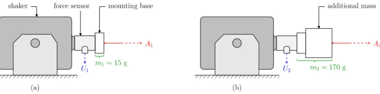
the calibration setup described in this appendix is taken from Marcos Pinho’s PhD work [29]. The calibration procedure consisted of two steps. First, the sensor was equiped with a mounting base of mass m1 = 15 g (Fig. A.1(a)).
The shaker was driven with a chirp in the range [100-6400] Hz and the velocity of the moving mass was measured using the laser vibrometer. A frequency re-sponse R1 corresponding to acceleration A1 over sensor output voltage U1 was
thereby obtained. Then, an additional mass was fixed to the mounting base (total mass m2 = 170 g, Fig. A.1(b)) and the same experiment was repeated
to obtain frequency response R2.
00000000000
11111111111 000000000000111111111111
A1 A2
shaker for esensor mountingbase additionalmass
U2 U1 m1
= 15g
m2= 170g
(a) (b)
Fig. A.1. Setup for the calibration of the force sensor.
Considering the moving mass as a rigid body and assuming pure transla-tional motion, the force measured by the sensor at each step is
Fi = (mi+ ms)Ai i∈ {1, 2}, (A.1)
where ms is the unknown moving mass in the sensor. If SF denotes the
un-known sensitivity of the sensor (in V/N), Eq. (A.1) may be written as
Ri = Ai Ui = 1 (mi+ ms)SF i∈ {1, 2}. (A.2) Using the two frequency responses R1 and R2 obtained with known masses
m1 and m2 respectively, it is possible to determine the sensitivity SF and the
internal moving mass ms of the sensor :
SF = 1 m2− m1 ( 1 R2 − 1 R1 ) and ms = R2m2− R1m1 R1− R2 . (A.3)
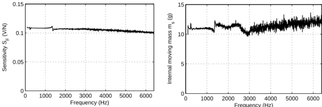
Figure A.2 shows the results of the calibration procedure. The sensitivity curve is comprised between 0.10 and 0.11 V/N, which is consistent with the value given by the manufacturer (111.6 mV/N). The internal moving mass is comprised between 10 and 13 g. The low-frequency value of 11 g may be retained.
B Correction of the measured force
In the experiment of Section 2, the force measured by the sensor is not directly the external force applied to the plate. It also includes an inertial force proportional to the sensor’s acceleration, due to the mass ms comprised
between the sensor and the plate. To obtain the net force exerted on the plate, the inertial force−ω2w(xF, yF)ms has to be removed from the measured force.
As the excitation point (xF, yF) does not coincide with one of the mesh points,
0 1000 2000 3000 4000 5000 6000 0 0.05 0.1 0.15 Frequency (Hz) Sensitivity S F (V/N) 0 1000 2000 3000 4000 5000 6000 0 5 10 15 Frequency (Hz)
Internal moving mass m
s
(g)
Fig. A.2. Sensitivity and moving mass of the force sensor obtained by the calibration procedure.
∆′ = ∆/10) using bicubic interpolation. Then, the location of the maximum of the rms force distribution in the neighbourhood of the external source pro-vides an accurate estimation of the excitation coordinates (xF, yF). Finally,
the displacement field at each frequency is also interpolated to estimate the displacement w(xF, yF) at the excitation point.
Figure B.1 shows the effect of removing the inertial force from the force measured by the sensor. The value of mass ms was adjusted to obtain the
best match between the corrected force measurement and the force identified with CFAT (see Fig. 6). A value of 10.2 g was found, which is of the same order as the internal mass of the sensor obtained from calibration.
0 1000 2000 3000 4000 5000 6000 −70 −60 −50 −40 −30 Frequency (Hz) Force (dB ref 1 N)
Fig. B.1. Force measured by the sensor, before (dashed blue) and after (solid black) removing the inertial force of the moving mass.
References
[1] C. P´ezerat and J.-L. Guyader. Two inverse methods for localization of external sources exciting a beam. Acta Acustica, 3:1–10, 1995.
[2] D.U. Noiseux. Measurement of power flow in uniform beams and plates. Journal of the Acoustical Society of America, 47(1 (Part 2)):238–247, 1969.
[3] G. Pavic. Measurement of structure borne wave intensity, part 1 : Formulation of the methods. Journal of the Acoustical Society of America, 49(2):221–230, 1976.
[4] C. P´ezerat and J.-L. Guyader. Force analysis technique: Reconstruction of force distribution on plates. Acustica united with Acta Acustica, 86:322–332, 2000. [5] M.S. Djamaa, N. Ouella, C. P´ezerat, and J-L. Guyader. Reconstruction of a
distributed force applied on a thin cylindrical shell by an inverse method and spatial filtering. Journal of Sound and Vibration, 301:560–575, 2007.
[6] M.S. Djamaa, N. Ouella, C. P´ezerat, and J-L. Guyader. Mechanical radial force identification of a finite cylindrical shell by an inverse method. Acta Acustica, 92(3):398–405, 2006.
[7] C. Renzi, C. P´ezerat, and J.-L. Guyader. Vibratory source identification by using the finite element model of a subdomain of a flexural beam. Journal of Sound and Vibration, 332(3):545 – 562, 2013.
[8] C. Renzi, C. P´ezerat, and J.-L. Guyader. Force identification on flexural plates using reduced finite element models. Computers and Structures (Accepted for publication), 2015.
[9] F. Chevillotte, Q. Lecl`ere, N. Totaro, C. P´ezerat, P. Souchotte, and G. Robert. Identification d’un champ de pression pari´etale induit par un ´ecoulement turbulent `a partir de mesures vibratoires. In Soci´et´e Fran¸caise d’Acoustique SFA, editor, 10`eme Congr`es Fran¸cais d’Acoustique, pages –, Lyon, France, 2010. [10] D. Lecoq, C. P´ezerat, J.-H. Thomas, and W.P. Bi. Extraction of the acoustic component of a turbulent flow exciting a plate by inverting the vibration problem. Journal of Sound and Vibration, 333(12):2505 – 2519, 2014.
[11] N. Totaro, C. P´ezerat, Q. Lecl`ere, F. Chevillotte, and D. Lecoq. Identification of boundary pressure field exciting a plate under turbulent flow. In FLINOVIA, Rome, Italie, November 2013.
[12] Y. Zhang and J.A. Mann III. Examples of using structural intensity and the force distribution to study vibrating plates. Journal of the Acoustical Society of America, 99(1):354–361, 1996.
[13] Y. Zhang and J.A. Mann III. Measuring the structural intensity and force distribution in plates. Journal of the Acoustical Society of America, 99(1):345– 353, 1996.
[14] Yi Liu and W. Steve Shepard Jr. An improved method for the reconstruction of a distributed force acting on a vibrating structure. Journal of Sound and Vibration, 291(1-2):369 – 387, 2006.
[15] A. Fregolent and A. Sestieri. Force identification from vibration measurements in the wavenumber domain. In Proceedings of ISMA 21, Leuven, Belgium, 1996. [16] Q. Lecl`ere, F. Ablitzer, and C. P´ezerat. Identification of loads of thin structures with the corrected Force Analysis technique: An alternative to spatial filtering regularization. In Proceedings of ISMA 2014, pages –, Leuven, Belgique, 2014.
[17] Q. Lecl`ere and C. P´ezerat. Vibration source identification using corrected finite difference schemes. Journal of Sound and Vibration, 331(6):1366 – 1377, 2012. [18] D.J. Ewins. Modal Testing: Theory and Practice. Engineering dynamics series.
Research Studies Press, 1986.
[19] J.G. McDaniel, P. Dupont, and L. Salvino. A wave approach to estimating frequency-dependent damping under transient loading. Journal of Sound and Vibration, 231(2):433 – 449, 2000.
[20] Y. Liao and V. Wells. Estimation of complex modulus using wave coefficients. Journal of Sound and Vibration, 295(1-2):165 – 193, 2006.
[21] C. Chochol, S. Chesne, and D. Remond. An original differentiation tool for identification on continuous structures. Journal of Sound and Vibration, 332(13):3338 – 3350, 2013.
[22] N.S. Ferguson, C.R. Halkyard, and B.R. Mace. The estimation of wavenumbers in two-dimensional structures. In Proceedings of ISMA 2002, pages 799–806, Leuven, Belgique, 2002.
[23] M.N. Ichchou, O. Bareille, and J. Berthaut. Identification of effective sandwich structural properties via an inverse wave approach. Engineering Structures, 30(10):2591 – 2604, 2008.
[24] J. Berthaut. Contribution `a l’identification large bande des structures anisotropes. Application aux tables d’harmonie des pianos a queue. PhD thesis, Ecole Centrale de Lyon, 2004.
[25] F. Ablitzer, C. P´ezerat, J.-M. G´enevaux, and J. B´egu´e. Identification of stiffness and damping properties of plates by using the local equation of motion. Journal of Sound and Vibration, 333(9):2454 – 2468, 2014.
[26] C. P´ezerat and J.L. Guyader. Identification of vibration sources. Applied Acoustics, 61(3):309 – 324, 2000.
[27] J.S. Bendat and A.G. Piersol. Engineering applications of correlation and spectral analysis. Wiley-Interscience, New York, 1980.
[28] Q. Leclere. Multi-channel spectral analysis of multi-pass acquisition measurements. Mechanical System and Signal Processing, 23:1415–1422, 2009. [29] M. Pinho. Comportement statique et dynamique d’une suspension de
![Fig. 2. Structural parameter estimated at each point, averaged in the frequency range [1 5] kHz](https://thumb-eu.123doks.com/thumbv2/123doknet/14379783.505752/11.892.190.713.734.1003/fig-structural-parameter-estimated-point-averaged-frequency-range.webp)
![Fig. 5. Identified load distribution (N/m 2 , in dB ref 1N/m 2 , display dynamic 35dB) integrated in [.5 6] kHz](https://thumb-eu.123doks.com/thumbv2/123doknet/14379783.505752/14.892.175.703.425.701/fig-identified-load-distribution-ref-display-dynamic-integrated.webp)