A non-stationary index resulting from time and frequency domains

HAL Id: hal-00381420

https://hal.archives-ouvertes.fr/hal-00381420

Submitted on 5 May 2009

HAL is a multi-disciplinary open access archive for the deposit and dissemination of sci-entific research documents, whether they are pub-lished or not. The documents may come from teaching and research institutions in France or abroad, or from public or private research centers.

L’archive ouverte pluridisciplinaire HAL, est destinée au dépôt et à la diffusion de documents scientifiques de niveau recherche, publiés ou non, émanant des établissements d’enseignement et de recherche français ou étrangers, des laboratoires publics ou privés.

A non-stationary index resulting from time and

frequency domains

Nadine Martin, Corinne Mailhes

To cite this version:

Nadine Martin, Corinne Mailhes. A non-stationary index resulting from time and frequency domains. CM 2009 - MFPT 2009 - 6th International Conference on Condition Monitoring and Machinery Failure Prevention Technologies, Jun 2009, Dublin, Ireland. �hal-00381420�

A non-stationary index resulting from time and frequency domains

Nadine Martin et Corinne Mailhes* GIPSA-lab, INPG/CNRS Department Images Signal

Grenoble Campus

BP 46 - 961, rue de la Houille Blanche F-38402 Saint Martin d'Hères – France

Phone 33 (0)4 76 82 62 69 Fax 33 (0)4 76 57 47 90

[email protected]

*IRIT-TESA, INP – ENSEEIHT 2, rue Charles Camichel

B.P. 7122

31071 Toulouse Cedex 7 – France

Abstract

Detecting the presence of non-stationarity events in a signal is a challenge that is still not taken up. The aim of this paper is to make a contribution to this key issue. We already proposed a non-stationarity detection defined in time-frequency domain in order to control the invariance of the time-frequency statistics. In this paper, in order to be not limited by the time and frequency resolution of a time-frequency approach, we propose another test in frequency domain. In frequency domain, the problem can be cast by taking advantage of the normalized-variance properties of a spectral estimator when analyzing non-stationary signals. This second test will confirm, invalidate or detect new frequency localizations of non-stationarities. Finally, the main contribution of the paper is to propose a stationary index defined so as to merge the information given by these two tests and to allow an alarm to be raised for a high level of non-stationarities. Applications on real-world signals show the pertinence of this new index.

1. Introduction

When processing signals, knowing that the underlying physical phenomena are non-stationary is of the first importance. Moreover, lots of processing methods rely on a stationarity assumption, which could be useful to test before any analysis. The aim of this paper is to propose a full methodology, for testing this stationarity assumption without any a priori hypothesis about the nature of the possibly non-stationarity events. In order to be of practical use, the methodology proposed will conclude with an index ranged between 0 and 100 so as to evaluate a level of non-stationarity.

2

In many applications, and above all in condition monitoring, Fourier analysis and spectrograms are standard and powerfull tools for studying time-varying signals. Great progress has been made in this area in order to improve resolution but this last point is not of importance when the issue is not to estimate and to detect. In addition, the main advantages of these classical transforms are their robustness and the fact that statistical properties are theoretically well known, which is of the first concern for this study. Finally, devising tests from these signal representations is motivated by the TetrAS project, in which signal-processing tools are developed around Fourier-based transforms (http://www.gipsa-lab.inpg.fr/index.php?id=304) and in which takes place this work. According to the definition of the stationarity of a process, a stationarity test should result in the control of its statistical properties versus time. Such an approach first requires a time-observation scale. The time-observation scale will be set by the time resolution of the time-frequency representation, which will infer the definition of the minimal size of the non-stationary event the test would be able to detect. This size becomes then an a priori assumption. Second, in order to control the process statistics, this approach needs a way of measuring and tracking either the probability law parameters, or the moment invariance. The tests proposed in this paper completes the one presented in a previous publication(1) and will be limited to the second order. Lastly, the methodology aims at estimating also both time and frequency locations of each nonstationary occurrence detected. Casting a test in a time-frequency domain plan is obviously well-fitted for solving this localization problem.

Early papers on the subject (see (1) for the references) deal with optimal criterions, which rules out the time-frequency interest, deal with methods adapted to some particular event detection as certain transients, or need a preliminary training data set. More recently, a method based on surrogates, stationarized data get from the data itself in order to get rid of a well-defined structuration in time(2), do not seem to be well-adapted to mixed signals. Its current implementation needs a number of choices, that the method proposed in this paper tries to avoid. Although the test gives also a final index, no time-frequency localizations are provided.

This paper is organized as follows. Section 2 describes the framework of this study. In section 3, the test proposed in (1) is recalled whereas a new test is elaborated upon. In section 4 a classification based upon a signal non-stationarity level is proposed from an original index computed with the proposed tests. In all of the sections, the performance of the methodology is dicussed around a number of real-world signals. Finally, Section 5 looks at the conclusions that can be drawn from the work.

2. Framework

Let x n

[ ]

be a discrete time signal of length N and frequency sampling Fs. The

observation set Lk_x

[ ]

n _{is a subset of} 2

R so that

[ ]

{

( )

2

[ ]

}

, / , and for a given

k

x n = n k ∈ ∃S n kx k

3

with k the frequency variable and S n k_x

[ ]

, a time-frequency representation of x n

[ ]

. As such, Lkx

[ ]

n includes a cross-section of S n kx

[ ]

, at a constant frequency k. The

time-frequency estimator is either a spectrogram,

[ ]

1

[ ] [

]

2 2 jk / 0 1 , e N m K x m s S n k x m w m nD N F π − − = =

∑

− , (2)

with w m

[ ]

a time window, D the window time-shift and K being the Fourier bin number, or a gliding correlogram evaluated from a biaised autocorrelation estimate,

[ ]

1 1

[ ] [

*

]

( )

2 jk / 0 1 1 , e N N m K x m u m s S n k x u x u m w m F N π − − − = =   =  −   

∑

∑

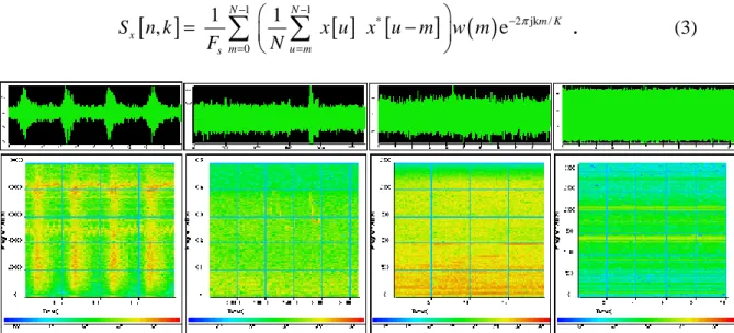
. (3)

Figure 1. Time signals and their spectrograms (with segment length equal to the close power of 2 of 2 % signal length, 50%overlapping, no zero padding and

Hanning window), (from left to right) a magnetic Barkhausen noise, dolphin whistles, a boat passing and gearbox vibrations.

Figure 1 shows time-frequency representations of four signals with segment length equal to the close power of 2 of 2 % signal length, 50% overlapping, no zero padding and Hanning window. The first one is a magnetic Barkhausen Noise (Fs=200 KHz over

0.2 s) measured with a magnetoresistive magnetic field sensor in order to evaluate the microstructure and the stress behaviour of ferromagnetic steels (3), the second one is a bioacoustic signal (Fs=15 364 Hz over 17.64 s ) measured with an hydrophone in order

to characterize dolphin whistles (4), the third one is an acoustic signal (Fs=5 KHz over

20 s after a decimation by a factor 4) measured with an hydrophone during a boat passing, and the fourth one is a vibratory signal (Fs=6 365 KHz over 10.3 s) measured

with an accelerometer on a test bench in order to identify vibrations induced by a gearbox.

[ ]

k x n

L _{is then an horizontal line at frequency k in each spectrogram of Figure 1for n} varying from 1 to P, the number of signal-windows. The union of sets Lkx

[ ]

n , with k

4

varying from 1 to K, contains all the time-frequency points of a spectrogram. The aim of the tests proposed is to extract from these sets a sub-set, which will contain all the points corresponding to non-stationary events. Proceeding with detection theory is then possible thanks to the use of Fourier-based transforms.

3. Two non-stationary detection tests

The definition of a stationary process excuses for the nonexistence of an unique efficient test. An ergodic random process is completely stationary if its probability density function remains unaltered under a time shift. This definition is a severe requirement and should be relaxed. Many tests were derived according to the way you relax. In a previous paper of the authors (1), a time-frequency test was proposed. Being used in the final section, this test will be summed up in this section. Then, using the result of this time-frequency test, a second test based on the signal spectrum only will confirm, refute or eventually detect other types of non-stationarities. It will be the subject of the second sub-section.

3.1 Time-frequency test

As we did in (1), let us define two hypotheses:

- H0 where the signal x n

[ ]

is equal to b n

[ ]

, a stationary random process with zero

mean, constant variance and time-frequency estimation S n k_b

[ ]

, , eventually added with a stationary deterministic signal d n

[ ]

with time-frequency estimation S_d

[ ]

n k, ; and where

[ ]

0 k H n L _{is defined as}

[ ]

{

( )

[ ]

(

[ ]

)

}

0 , / x 0 0 , min for a given

H k = n k ∈ x k pS H = p et E S n kx k

L L _{, (4)}

with S n k_x

[ ]

, distributed as gamma Γ

(

_r 2,

α

, 0

)

_{,which defines} 0

p , the probability density function of S n k_x

[ ]

, under this hypothesis. See (6) for further details about the chi-square approximation.

- H1 where x n

[ ]

is nonstationary and where LkH₁

[ ]

n is by definition the complement

of

[ ]

0

k H n

L _.

The two parameters of the law p₀, parameter r, the equivalent degree of freedom, and parameterα are defined as,

[ ]

(

)

(

(

[ ]

)

)

(

(

[ ]

)

)

[ ]

(

)

(

)

2 2 2 E , E , ₂ Varn , = r , x x x x S n k S n k S n k E S n k − = and α= E S k

(

b

[ ]

,ν

)

r, (5) with Varn

(

S n k_x

[ ]

,

)

the normalized variance of the observation. The first moment about zero of S n k_b

[ ]

, , E S k

(

b

[ ]

,ν

)

, can be estimated from the average of the points

5

belonging to

[ ]

0

k H n

L _{, which allow} α _{to be estimated as,}

[ ]

₍

_{[ ]}

₎

[ ]

[ ] 0[ ] 0 / , 1 ˆ , b H b n S n k k H α _{k S n k r} card k ∈ =

∑

L L , (6)

[ ]

ˆ

α _{k being an estimation of} α _{at frequency k .}

As a matter of fact, if a deterministic signal d n

[ ]

is eventually present under H0,

[ ]

,

x

S n k is proportional to a noncentral chi-square variable,

χ δ

'r2'

( )

, with the same proportionality parameter α , a degree of freedom r', and with noncentrality parameter

[ ] [ ]

' _d , _b , r S n k S n k

δ

= . In this case, the normalized variance,

[ ]

(

)

(

₍

₎

2

)

2 ' 4 Varn , ' x r S n k r

δ

δ

+ = + . (7)

depends on the method parameters and mostly on the deterministic signal, whether the estimator is either a spectrogram or a correlogram. Nevertheless, the normalized variance in (7) is always lower than the normalized variance in (5). So, if we use the gamma distribution of the only-noise case in a detection test instead of the non-central chi-square distribution, the detector will always work but the real Pfa will be lower. Afterwards, considering p as equal to a gamma law as in (4), we can write at each ₀

frequency k the decision rule,

[ ]

[ ] [ ] [ ] [ ]

[ ]

[ ] [ ]

1 1 0 1 , , ˆ , k x H k r H H is true S n k n x Pfa Pfa H is true S n k n S n k η k λ k α k ∈ ∈ > _{= ×} < L L , (8)

which allows making a decision between the two hypothesis H0 and H1. Knowing that a

gamma variable is proportional to a chi-square one χr2, a given probability of false

alarm Pfa has permitted the calculation of the detection threshold

η

_Pfa

[ ]

k after inverting the following integral,

[ ] [ ] [ ]

( )

2 2

1

r r

Pfa k Pfa k Pfak

s Pfa _αg_χ ds g_χ u du η

α

λ η α +∞ +∞ =   =   =  

∫

∫

, (9) where 2

( )

r

g_χ u is the probability density function of a 2

r

χ

. The threshold

λ

_Pfa

[ ]

k is equal to 1 minus the Pfath-quantile of a 2

r

6

partition of Lk_x

[ ]

n _{being unknown, an iterative algorithm is proposed to be able to apply} this decision rule. See (1) for more details.

The result of this test is represented as a time-frequency map. Each element of

[ ]

1

k H n

L _is coded by the normalized value S n k_r

[ ]

,

λ

_Pfa

[ ] [ ]

k

α

ˆ k , whose maximum value is 1, and all elements of

[ ]

0

k H n

L _{are coded by 0. In an alternative map, each element of}

[ ]

1

k H n

L _is classified according to the value of Pfa that detects this element at the last iteration. Each class is defined as

(

)

[ ]

[ ]

[ ] [ ]

[ ]

1

[ ]

1 1 _{ˆ ˆ} Class = , / c , c c c k I I x H _Pfa x _Pfa k

Pfa Pfa Pfa S n k n λ k α k S n k λ α+ k

+ ≤ <  ∈ ≤ <  

∪

L  (10) with c Pfa and c 1

Pfa + successive values of c

Pfa in the Pfa set defined as

{

10 ,10 ,10 ,10−2 −3 −4 −5

}

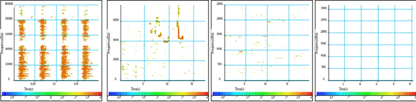
, and which defines 5 classes.

Figure 2. Results of the time-frequency test applied on spectrograms computed with (from left to right) the magnetic Barkhausen noise, the dolphin whistles, the

boat passing and the gearbox vibrations. Horizontal axis is time in s whereas vertical axis is frequency in Hz.

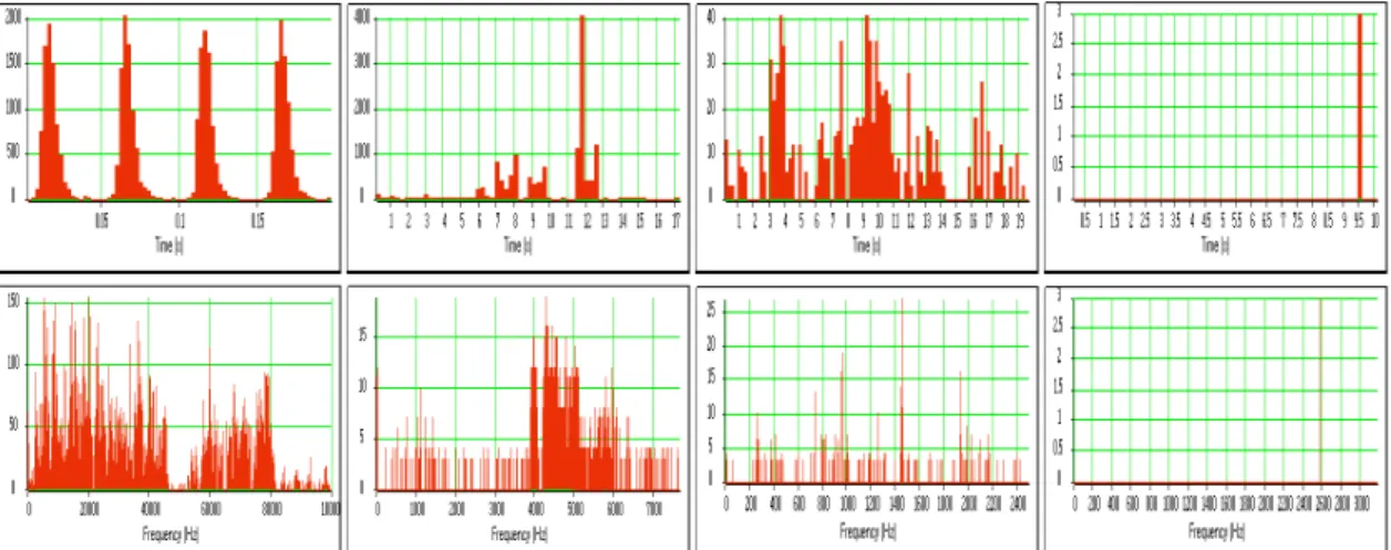
This time-frequency test was applied to signals of Figure 1with a false alarm probability equal to 10-4. Figure 2 shows the map defined by (10) for each signal. Figure 3 shows time projections, referred to as

[ ]

1

H

P n , and frequency projections, referred to as

[ ]

1 H P k , defined as

[ ]

[ ]

[ ]

(

[ ]

)

1 1 1 1 , . k H H k k H H P n card n P k card n   =     =

∪

L L (11)

The transient structures of the Barkhausen noise are well detected whereas the stationary narrow-band frequencies present all over the time duration of the signal (close to 30 kHz and 50 kHz) are fortunately undetected. These frequencies may come from some external interferences of the measurement equipment. In this application,

7

this test has performed a source separation in the time-frequency domain. In the second signal, the non-stationary parts of the signal, the dolphin whistles are very well localised in the submarine noise. In the third signal, the signal is globally stationary apart a very localized frequency event corresponding to amplitude modulations in a band around 1 450 Hz. This band is well marked in the frequency projection, see Figure 3. The last signal is totally stationary, except for one non-significant point.

Figure 3. Time projection in s (up) and frequency projection in Hz (bottom) of the detection map get with the time-frequency test applied on the four studied signals, (from left to right) the magnetic Barkhausen noise, the dolphin whistles, the boat

passing and the gearbox vibrations.

3.2 Normalized variance test

To round out the time-frequency test, a second test limited to second order also is designed in the frequency domain only.

In the previous sub-section it was noticed that, first, the normalized variance of a spectrum for a noise-only signal is constant (see (5)), and second, this variance is lower when a deterministic signal being present (see (7)). Furthemore, if a signal contains a non-stationarity at a frequency, this variance increases and if the non-stationarity is high, the variance will exceed its variations due to its own variance. These properties are tolerant vis-à-vis the Gaussian noise assumption. A test based on a normalised variance could then be able to detect non-stationary events.

The test proposed in this section aims at detecting the high variations of the normalized variance according to a stationary case. Based upon the previous time-frequency test and the definition of the normalised variance recalled in (5), the frequency test of this section is defined as

[ ]

[ ]

[ ]

[ ]

1 2 2 1 0 2 0 1 ˆ ˆ ˆ ˆ P _H p x p P s H k k P varn k k γ µ ζ µ − = − > = <

∑

(12)

8

with

γ

ˆp

[ ]

k =Sx

[ ]

p k, the spectrum estimate over the p th

signal window (see (2)), P the number of signal-windows in equation (2), and where

µ

ˆ_x

[ ]

k ,

[ ]

₍

_{[ ]}

₎

[ ]

[ ] 0 0 1 ˆ ˆ k H x _k p p n H k k card n

µ

γ

∈ =

∑

L L , (13)

results of the previous test and is the mean value of

[ ]

0

k H n

L _{set. Indeed, the previous test} provides the P independent estimations of the spectrum

γ

ˆ_p

[ ]

k required in (12). Theoretically, varnˆ _P

[ ]

k is then equal to a constant depending on the window shape and of the average number.

γ

ˆ_p

[ ]

k is estimated with a Blackman window and without averaging due to the time-frequency estimator, then varnˆ _P

[ ]

k in (12) is equal to 1 when using a spectrogram (from (2) and r=2 from (5)) or 0.49 when using a correlogram (from (3) and r=4.08 from (5)).

The threshold ζ should be defined from the standard deviation of varnˆ _P

[ ]

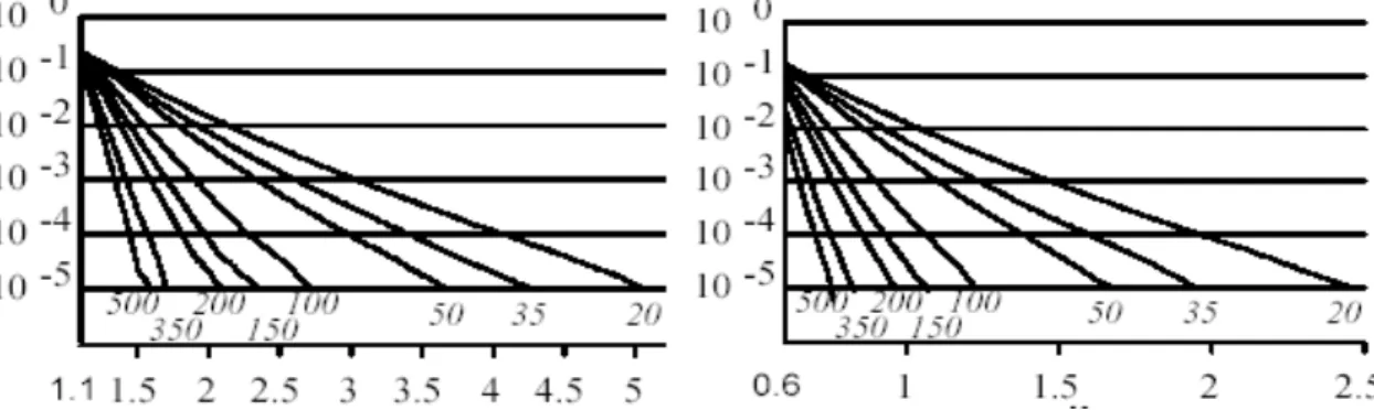
k considered as a random process. As the derivation of the confident interval is a tricky task, a simulation procedure with 20 000 runs of a white Gaussian noise has determined the value of the threshold ζ according to the false alarm probability Pfavarnorm and the signal-window number P.

Figure 4. Simulation results of the normalised variance of a spectrum estimated by spectrograms (on the left) or gliding correlograms (on the right) versus the probability of false alarm Pfavarnorm (vertical axis) and the threshold ζ (horizontal

axis) and the signal-window number P (number over the figure)

Figure 4 shows the results for both the spectrogram and the gliding correlogram. Table 1 makes use of the simulation results and suggests a final choice of the threshold ζ for different ranges of the signal-window number P and for 4 values of the false alarm probability Pfavarnorm. It is important to notice that the value of P will lie in the range [30,150] due to the fact that, in the time-frequency test proposed, the length of the signal-window is fixed to the close power of 2 of 2 % signal length with 50%

9

overlapping.

Table 1. Choice of the detection threshold in the normalized variance test according to the simulation process and for both the spectrogram and gliding

correlogram.

Spectrogram Gliding correlogram

P Pfavarnorm from20 to 30 from 30 to 70 from 70 to 150 from 150 to 400 > 400 from 20 to 30 from 30 to 70 from 70 to 150 from 150 to 400 > 400 10-5 5 3,7 2,5 2 1,6 2,4 1,7 1,3 1 0,8 10-4 4 3 2,3 1,8 1,5 1,9 1,4 1,1 0,9 0,75 10-3 3 2,4 2 1,6 1,4 1,4 1,2 1 0,8 0,7 10-2 2 1,8 1,6 1,4 1,2 1 0,9 0,8 0,7 0,6

Figure 5 shows the results for the dolphin whistles and, in particular, the stationary spectrum estimated by the first time-frequency test. The normalized variance shows that the variance is around 1 for most of the frequencies excepted for the frequency band containing the dolphin whistles, so the non-stationary part of the signal.

Figure 5. Detailed results of the normalized variance test applied to the spectrogram of the dolphin whistle signal (the second signal), (left, up to bottom) spectrum

γ

ˆ_p

[ ]

k with P=65, mean value

µ

ˆ_x

[ ]

k of

[ ]

0

k H n

L _{from time-frequency-test,}

(right, up to bottom) normalised variance varnˆ _P

[ ]

k with Pfavarnorm=10-4 then

threshold ζ =3 in green dotted line, frequency alarm plot V[k].

The last plot shows the frequency alarms referred to as V[k] and given by

[ ]

[ ]

[ ]

[ ]

10 ˆ 0 if ( ) . ˆ 1 if ( ) P P V k varn k H V k varn k H

ζ

ζ

= ≤ = > (14)

Figure 6 shows the results for the three other signals. The magnetic Barkhausen noise is non-stationary for almost all the frequencies, which confirms the result of the

time-10

frequency test (see Figure 3). For the boat passing signal, alarms are not all confirmed and some new frequencies are detected. More insights are necessary in this case, which will be the purpose of the next session. The gearbox vibration signal is totally stationary, no point of the variance exceeds the threshold, even the non-significant point of the first test, which is then not confirmed. This last example is interesting for the normalised variance shows several points well below 1, which characterizes deterministic components in the signal, which is indeed the case.

Figure 6. Results of the normalized variance test with Pfavarnorm=10-4 applied to the

spectrogram of the three other signals, (left to right) the magnetic Barkhausen noise with P=77 then ζ =2.3, the boat passing with P=96 then ζ =2.3, the gearbox vibrations with P=63 then ζ =3, (up to bottom) normalised variance varnˆ _P

[ ]

k with

threshold in green dotted line, frequency alarm plot V[k].

4. Classification from a stationary index

After having proposed tests, a final indicator is necessary in order to merge the information given by the two tests and also to provide one numerical index, which will allow a quick decision just after the signal acquisition. This index is targeted to assess the occurrence of non-stationary events without any considerations about their nature, then their time-frequency shape.

In that context, several indexes are defined. The first two merge the results of the time-frequency detection map defined in (10) by calculating the detection number referred to as Nbdet_time and Nbdet_freq and a percentage referred to as %det_time and %det_freq in

the time and frequency projections

[ ]

1

H

P n and

[ ]

1

H

P k defined in (11), that is to say [ ] [ ] 1 1 det_ det_ 1, det_ det_ 1, 0 and % _ = × 100 / , 0 and % _ = × 100 / , H H P n time time n P P k freq freq k K Nb P det time Nb P Nb K det freq Nb K = = = − = −

∑

∑

(15) with ₀PH1[ ]n and ₀PH1[ ]k

, zero to the power

[ ]

1

H

P n and

[ ]

1

H

P k respectively, providing the number of zero values in vectors

[ ]

1 H P n and

[ ]

1 H P k respectively.

11

The following three convey the contribution of the normalized test according to the time-frequency test, [ ]

(

)

[ ]

[ ]

_{[ ]}

[ ]

(

)

(

[ ]

)

1 1 1 _ _ 1, _ _ 1, _ _ 1, = 1 0 and % _ = 100 / , = 0 and % _ = 100 / , 1 0 1 and % _ = H H H P k

conf freq conf freq

k K

P k

new freq news freq

k K P k fa freq fa freq k K Nb V k conf freq Nb K Nb V k new freq Nb K Nb V k fa freq Nb = = =  _{− ×}  _×      _×  _×     = _ − × − _ ×

∑

∑

∑

100 / , . K (16) where

(

_{1 0}− PH1[ ]k

)

is a binary-value vector deduced from

[ ]

1

H

P k and ₀PH1[ ]k the orthogonal one. The product

(

_{1 0}PH1[ ]k

)

[ ]

V k

 _{− ×} 

 

  between the two binary vectors gives

the detections confirmed referred to as conf_freq. When the first is replaced by its orthogonal, the product gives the new detections referred to as new_freq and the product between the two orthogonal vectors referred to as fa_freq gives the false alarms, that is to say the detections non-confirmed by the second test.

The stationary index proposed is then defined by

_ _ % _ % _

Stat index time− freq = det time × Rev det freq, (17) with %det time from (15) and _ Rev detect% _ freq defined as

(

_ _ _

)

% _ _{det freq new freq fa freq} 100 / ,

Rev det freq = Nb +Nb −Nb × K (18)

a revision of the index %det_ freq in order to take both tests into account.

Finally, the redundancy between the two tests is expressed by

(

)

_ _ _

_ _{conf freq} 100 / _{det freq new freq} ,

Redondancy freq =Nb × Nb +Nb (19)

Table 2. Values of the indexes proposed for the four studied signals

%det_time %det_freq %conf_freq %new_freq %fa_freq Rev%det_freq

Barkhausen 72,7% 81,3% 76,6% 1,4% 4,7% 78,0% 56,7% 92,7% Dolphin 76,9% 24,9% 18,7% 0,0% 6,2% 18,7% 14,4% 75,1% Boat 70,8% 9,9% 2,0% 0,0% 7,8% 2,1% 1,5% 20,7% Gearbox 1,6% 0,1% 0,0% 0,0% 0,1% 0,0% 0,0% 0,0% Redondancy_ freq Signal

t-f test Normvar test % t-f test

Stat_index_ti me-freq

12

paper. Finally, relying upon a wider data base analysis, a symbolic classification is proposed and defined as

_ _ 0%

0% _ _ 4% !

4% _ _ 16% !!

_ _ 16% !!!

Symbolic Classification

Stat index time freq Stationary

Stat index time freq Warning

Stat index time freq Serious warning

Stat index time freq Alarm

− =

< − ≤

< − ≤

− >

. (20)

The last class corresponds, for example, to 40% time detection and 40% frequency detection in the time-frequency map, which is without any doubt a case of alarm relatively to the stationarity of the signal. Including this classification, Table 3 compares the results obtained with an expert interpretation. For the four studied results the stationary index proposed performs well.

Table 3. For the four studied signals, comparison of the stationary index proposed with an expert interpretation

Magnetic Barkhausen Noise 56,7% Alarm!!! Strongly Non-Stationary

Dolphin Whistles 14,4% Serious Warning!! Non-Stationary, Presence of non-linear modulations locally

Boat Passing 1,5% Warning! Non-Stationary, small variations of central frequencies of narrow band patterns & small amplitude variations

Gearbox Vibrations 0,0% No Alarm Stationary Stat_index_t

ime-freq Expert view Signal Classification given by the

tests

5. Conclusions

This paper has proposed a stationary index defined in percentage in order to characterize the presence of stationary events in a signal without taking the nature of theses stationarities into account. This index does not need high computations and is easily and fast computed from a spectrogram or a gliding correlogram of a signal. This test is of interest to control all signal acquisitions as a pre-analysis before applying more specific processing. It can also be used in order to localise the non-stationarities, which can be the input of some algorithms. Future works will include another time test in order to reinforce the time index as the normalized-variance test does for the frequency index.

References

1. N. Martin, A criterion for detecting nonstationary event. Special session, Twelfth International Congress on Sound and Vibration, ICSV12, Lisbonne, Portugal, July 11-14, 2005.

2. P. Borgnat, P. Flandrin, Stationarization via surrogates, J. Stat. Mech.: Th. and Exp., doi:10.1088/1742-5468/2009/01/P01001, 2009.

3. L. Padovese, F. Millioz, N. Martin, Time-frequency and Time-Scale analysis of Barkhausen noise signals. To appear in Journal Proceedings of the Institution of

13

Mechanical Engineers, Part G, Journal of Aerospace Engineering for the Structure and Machine Monitoring Special issue, 2009.

4. F. Millioz, J. Huillery and N. Martin, Short Time Fourier Transform Probability Distribution for Time-Frequency Segmentation. IEEE International Conference on Acoustics, Speech, and Signal Processing, Proceedings of ICASSP 2006, pp. III-448-451, May 14-19 2006.

5. N. Martin, Advanced Signal Processing and Condition Monitoring. International Journal Insight on Non-Destructive Testing and Condition Monitoring. Vol. 49. No 8, August 2007.

6. J. Huillery, N. Martin, On the Description of Spectrogram Probabilities with a Chi-quared Law. IEEE Transactions on Signal Processing, Vol. 56, Issue 6, June 2008