HAL Id: hal-01148252
https://hal.archives-ouvertes.fr/hal-01148252
Submitted on 4 Nov 2015HAL is a multi-disciplinary open access archive for the deposit and dissemination of sci-entific research documents, whether they are pub-lished or not. The documents may come from teaching and research institutions in France or abroad, or from public or private research centers.
L’archive ouverte pluridisciplinaire HAL, est destinée au dépôt et à la diffusion de documents scientifiques de niveau recherche, publiés ou non, émanant des établissements d’enseignement et de recherche français ou étrangers, des laboratoires publics ou privés.
Heat and strain measurements at the crack tip of filled
rubber under cyclic loadings using full-field techniques
J.R. Samaca Martinez, Evelyne Toussaint, X. Balandraud, Jean-Benoit Le
Cam, D. Berghezan
To cite this version:
J.R. Samaca Martinez, Evelyne Toussaint, X. Balandraud, Jean-Benoit Le Cam, D. Berghezan. Heat and strain measurements at the crack tip of filled rubber under cyclic loadings using full-field tech-niques. Mechanics of Materials, Elsevier, 2015, 81, pp.62-71. �10.1016/j.mechmat.2014.09.011�. �hal-01148252�
Heat and strain measurements at the crack
tip of filled rubber under cyclic loadings using
full-field techniques
J. R. Samaca Martinez
a,b,e, E. Toussaint
a,b, X. Balandraud
c,b,
J.-B. Le Cam
dand D. Berghezan
ea
Clermont Universit´e, Universit´e Blaise Pascal, Institut Pascal, BP 10448, 63000 Clermont-Ferrand, France
b
CNRS, UMR 6602, Institut Pascal, 63171 Aubi`ere, France
cClermont Universit´e, Institut Fran¸cais de M´ecanique Avanc´ee, Institut Pascal,
BP 10448, 63000 Clermont-Ferrand, France
dUniversit´e de Rennes 1, Institut de Physique de Rennes, UMR 6251, Campus de
Beaulieu, 35042 Rennes, France
eMICHELIN, CERL Ladoux, 63040 Clermont-Ferrand, France
Abstract
This study aims at characterizing heat sources during the deformation of the crack tip zone in carbon black filled Styrene Butadiene Rubber (SBR). For this purpose, the thermomechanical response of cracked specimens was investigated using coupled full thermal and kinematic field measurements and a suitable motion compensation technique. The kinematic analysis enabled us to define the zone of influence of the crack and to measure the maximum stretch ratio level. The maximum stretch ratio level at the crack tip is higher than that measured at specimen failure during
uniaxial tensile tests, which can be explained by considering the maximum chain extensibility. The calorimetric analysis shows that the high heat source gradient zone is very much more confined than the high temperature gradient zone. The heat sources at the crack tip remain positive and small during unloading, which indicates that mechanical dissipation is high and confined to the crack tip. This result highlights that the material behaves very differently in the crack tip zone compared to homogeneous tests. This proves that it not possible to predict the behavior of the crack tip zone from homogeneous tests. Moreover, it is observed that the mechanical dissipation decreases with the number of first cycles, which highlights the fact that the material is increasingly accommodated. This study provides the first accurate measurement of heat sources at the crack tip of rubber, constituting a new experimental tool in the fracture mechanics of rubber.
Key words: rubber - crack tip - thermomechanical analysis - infrared thermography - digital image correlation - quantitative calorimetry
1 Introduction
Elastomers are definitely one of the most versatile of materials, due to their entropic elasticity, their high damping properties, the nature of their thermal sensitivity, the ability of their filler network to reorganize, etc. These properties are all factors involved in mechanisms of deformation and damage, especially in high strain and stress gradient zones such as crack tips. More specifically as regards fracture mechanics in rubber, the tearing energy was defined by [1] as the large strain counterpart of the elastic energy release rate previously
1
Corresponding author Evelyne.Toussaint@univ-bpclermont.fr Fax : (+33) 473 405 381
proposed by [2]. This approach is still largely employed. The tearing energy is defined at the global scale by considering the balance of energy between the strain in a body and a crack. This is the total energy required to gener-ate a unit fracture surface in a purely elastic body. Nevertheless, a significant part of this energy is dissipated mechanically by viscous effects and possibly stress softening at the crack tip. This is the reason why temperature, loading rate and the global loading applied also have significant effects on the tearing energy [3, 4]. Consequently, the local measurement of mechanical quantities such as mechanical dissipation is of paramount importance to improve our knowledge and prediction of crack growth. The present study focuses on the measurement of heat sources, especially mechanical dissipation, at the local scale in the zone of influence of the crack. For this purpose, full-field mea-surement techniques were used. Even though these techniques have recently spread to investigate crack propagation in rubber (this aspect is reviewed in [5]), no study reports accurate measurements of heat sources at the crack tip of a rubber specimen. The present study aims to perform such measurements by using coupled kinematic and thermal field measurements. For materials undergoing large deformations, such as elastomers, one problem consists of tracking points that undergo large displacements at their surface. Digital im-age correlation is probably the most suitable technique that can be used to tackle this issue. Temperature variation fields can be measured at the speci-men surface using infrared thermography. As temperature fields are influenced by conduction as well as heat ex changes with ambient air and grips, it is not possible to distinguish heat sources due to the thermomechanical couplings (thermoelasticity, microstructural changes if any, etc.) from heat sources due to mechanical dissipation (viscosity, damage, etc.). This is the reason why we processed the temperature variation fields using a numerical strategy based
on the heat equation in order to calculate the heat sources (the reader can refer to [6] for further information). The paper is composed of three main parts. The first presents the experimental setup through the material for-mulation, the specimen geometry, the loading conditions and the full field measurement techniques. The second deals with image processing, including the motion compensation technique, the post-processing of the temperature fields and the heat source calculation. The third part presents the results and discussion. Concluding remarks close the paper.
2 Experimental setup
2.1 Material
The material was non-crystallizable styrene-butadiene rubber (SBR) filled with 50 parts per hundred of rubber in weight (phr) of carbon black. The ma-terial was cured for 22 min.The mould temperature was set to 150◦C. The glass
transition temperature was equal to -48◦C. Table 1 summarizes the chemical
composition of the rubber, whose molar mass was 120,000 g/mol. The ther-mal diffusivity D, which is involved in the heat diffusion equation in section 3.2.1, was equal to 1.81 10−7m2/s. The specific heat C
p ≈ CE, the
coeffi-cient of thermal expansion α and the thermal conductivity λ were equal to 1591 J.kg−1.K−1, 48.9 10−5K−1 and 0.317 W.m−1.K−1 at 25◦C, respectively.
Finally, the density ρ was equal to 1101 kg.m3
at the same temperature. The specimen, whose geometry was 80 mm wide, 2 mm thick and 13 mm high, is presented in Figure 1. It corresponded to classic Pure Shear (PS) geometry. It was notched on one of its sides using a razor blade. The initial crack length
was about 8 mm. This geometry corresponding to the undeformed state of the specimen was chosen as the reference configuration.
2.2 Loading conditions
The global mechanical loading corresponded to cyclic uniaxial loading. In the present study we focus on the effect of stress softening in the zone surrounding the crack tip. As this phenomenon occurs between the first and the tenth cycle in case of a homogenous tensile test (see Ref. [7]), ten mechanical cycles were applied. The first and the tenth cycles were analyzed. Moreover, as stress soft-ening mainly occurs between the first and second cycles, the second cycle was also analyzed. The global mechanical loading was applied under a prescribed displacement using a 500N INSTRON 5543 testing machine (see Figure 2). The signal shape was triangular in order to impose a constant global strain rate during loading and unloading. The displacement speed of the moving grip was equal to ± 200 mm/min. The maximum global stretch ratio, defined as the ratio between the current and initial lengths of the gauge zone, was equal to 1.5.
2.3 Full thermal and kinematic field measurements
Temperature field measurements were performed on one side of the specimen using a Cedip Jade III-MWIR infrared camera, featuring a focal plane array of 320 × 240 pixels and detectors with a wavelength range of 3.5-5 µs. Integration time was equal to 1500 µs. The acquisition frequency fa was set to 50 Hz. The
Non-Uniformity Correction (NUC) procedure. The thermal resolution, namely the noise-equivalent temperature difference (NETD), was equal to 20 mK. The spatial resolution of the temperature fields is the size of the pixel on the surface of the specimen. For the present test, it was equal to 62.5 µm. To ensure that the internal temperature of the camera was stabilized, it was switched on four hour before the experiment started. This camera temperature stabilization was necessary to avoid any drift in the measurements during the test. The thermal quantity considered in the present study was obtained by subtracting the initial temperature from the current one, after applying a suitable movement compensation technique used to track this zone during the test. For this purpose, the kinematic fields of the surface on the other side of the specimen were obtained using the Digital Image Correlation (DIC) technique [8]. This consists of correlating the grey levels between two different images of a region of interest (ROI) recorded using a cooled 16-bit PCO-Edge sCMOS camera. The acquisition frequency was set to 50 Hz. The sensor of the camera had 5.7 106
pixels (2160 x 2650). The methodology used enabled us to reach a resolution of 0.05 pixels, corresponding to 0.5 µm, and a spatial resolution (defined as the smallest distance between two independent points) of 10 pixels, corresponding to 101 µm. Uniform lighting at the specimen surface was ensured by a set of fixed lamps. The software used for the correlation process was SeptD [9]. A set of sub-images was considered to determine the displacement field of a given image with respect to a reference image. This set is referred to as the “Zone of Interest” (ZOI). A correlation function was used to calculate the displacement of the centre of a given ZOI between two images captured at different loading steps. Talc was deposited on the specimen surface before testing to improve the contrast of the images.
3 Image processing
Since the specimen undergoes large deformations, any given material point at its surface significantly moves during material deformation, while the zone captured by the detector array of the infrared camera remains fixed. A corre-spondence between the geometry of the specimen at any stage of the loading and the reference geometry must therefore be performed to obtain the tem-perature variation at any material point. This consideration has recently been addressed for various materials [10, 11, 12, 13, 14]. The next section briefly recalls how thermal fields measured in the deformed configuration are mapped in the reference configuration. More details can be found in [6].
3.1 Motion compensation technique
As mentioned above, two cameras are employed, on opposite sides of the sam-ple. The first camera enables us to determine displacement fields at the center of each ZOI on one side of the specimen. Fields can be represented either in the current or in the reference configuration. The second camera captures the temperature distribution on the opposite side and is therefore known in the current configuration. The correspondence between the two captured scenes is first performed, taking into account the size of the thermal and kinematic pixels. Displacement fields are then interpolated over the infrared camera grid. The deformed grid given by the DIC system is also interpolated on the ther-mal grid. The undeformed grid mapped onto the therther-mal grid is obtained by subtracting the displacement field interpolated on the thermal grid from that interpolated on the deformed thermal grid. The next step consists of
ting the temperature field in the reference coordinate system. This is done by combining the thermal and displacement fields, which are now known on the same grid. The above procedure is applied to the reference temperature map. Finally, the temperature field variations θ in the undeformed configuration is obtained by subtracting the initial temperature field from the current one.
3.2 Post-processing of temperature fields after motion compensation
This section explains how to obtain the heat source fields from the tempera-ture fields in the Lagrangian configuration. In this paper the term ’heat source’ means the heat power density (in W/m3
) which is produced or absorbed by the material. Moreover, ’heat source’ and ’heat’ must be distinguished: heat (in J/m3
) is the temporal integration of heat source. Processing is performed in the Lagrangian configuration, i.e. after applying the motion compensation described in the previous section. The calculation of heat sources is based on the heat diffusion equation. First the 2D version of the heat diffusion equa-tion is briefly recalled, then some practical informaequa-tion about the numerical processing is given.
3.2.1 Two-dimensional version of the heat diffusion equation
The heat diffusion equation which governs the temperature field in an isotropic material can be written as follows in the Lagragian configuration:
dT
dt − D0 ∆T =
S + R ρ0CE
(1)
the heat source produced by the material itself. The material parameters are the density ρ0, the specific heat CE at constant strain E and the thermal
diffu-sivity D0 (assumed to be isotropic in the Lagrangian configuration).
Temper-ature change θ is defined with respect to the reference temperTemper-ature Tref, i.e.
before starting the test: θ = T − Tref. If the external heat source rext remains
constant during the test, Equation 1 can be rewritten:
dθ
dt − D0 ∆θ = S ρ0CE
(2)
Let us consider a rubber specimen of small thickness in the Z-direction and loaded in the (X, Y ) plane. Assuming that the temperature change θ is almost homogeneous through the thickness, a 2D version of the heat diffusion equation can be written as follows [15, 16]:
dθ dt + θ τ − D0 ∆2Dθ = S ρ0CE (3)
where S = S(X, Y, t) and θ = θ(X, Y, t). In this equation, symbol ∆2D is the
Laplacian operator in the (X, Y ) plane; thus ∆2Dθ = ∂ 2
θ/∂X2
+ ∂2
θ/∂Y2
. Parameter τ is a time constant characterizing heat exchanges with the air by convection in the z-direction. Its value (40 s) was measured in [17].
The heat source S is expressed in W/m3
, whereas S/ρ0CE is in◦C/s. This last
quantity can be interpreted as the temperature rate that would be obtained in the case of adiabatic variation. In the following, S/ρ0CE will be still named
’heat source’ for the sake of simplicity. This unit is used for instance in Refs. [15, 14, 18, 19], which also consider heat sources divided by ρ0CE.
The heat source fields S/ρ0CE can be deduced from the temperature change
fields θ thanks to the left-hand part of Equation 3.
3.2.2 Practical aspects of heat source calculation
In this section, two practical points concerning the calculation of heat sources from temperature changes are discussed: (i) the problem of non-uniformity of the IR detector matrix in the case of large displacements of the material points, (ii) filtering/differentiation in the case of noisy data.
3.2.2.1 First practical aspect A specific problem appears when calcu-lating temperature changes in the case of large displacements of the materials points [10]. It is well known that a focal plane array IR camera is characterized by the non-uniformity of its detector matrix (see Refs. [20, 21]). The influence of this non-uniformity can be limited by performing a calibration with a black body. Whatever the result of this calibration, the temperature fields on a specimen captured by the camera may be altered by a parasitic non-uniform distribution denoted H (see Ref. [10]). The amplitude of this heterogeneity is usually very small (a few tenths of one degree). When the camera is run for several hours before being used for measurements, it can be checked that the parasitic field remains constant in time: H(i, j, t) = H(i, j) where (i, j) are the pixel coordinates in the image. This property is very useful in the case of small displacements of the material points. Indeed, when subtracting the reference temperature field Tref camera from the current temperature field Tcamera, both
being captured by the camera, the temperature difference is correctly mea-sured. In case of large displacements of the material points of the specimen, a specific procedure must be used. It consists of subtracting the field H from any temperature map Tcamera, including the reference one Tref camera, before
launching the motion compensation technique described above. With such a procedure, the temperature change fields θ are correctly measured. The reader can refer to Ref. [10] for a detailed demonstration and a validation test based on rigid-body movement.
3.2.2.2 Second practical aspect The calculation of heat sources con-sists of processing the left-hand side of Eq. 3. The main difficulty of this calculation is the fact that the temperature fields are unavoidably noisy. This increases errors in the values of the derivative terms dθ/dt and ∆2Dθ. Some
filtering strategies have been tested in the literature: mean-square approxima-tion [22], low-pass recursive filter [23], Fourier series [15], derivative Gaussian filter [24]... Filtering improves the resolution of the measurements, but deteri-orates the temporal resolution (in the case of temporal filtering) or the spatial resolution (in the case of spatial filtering). In particular, the diffusion term −D0∆2Dθ was slightly filtered in order not to penalize the spatial resolution.
This is important in the present case of a cracked specimen, for which a high temperature gradient is expected at the crack tip. The processing is done in two steps:
• step 1: filtering. Two averaging filters are used to smoothen the temperature change fields. In practice, they were applied using a convolution product with Matlab software [25]. A 1D kernel was used for filtering over time. A
2D kernel was used for filtering in the (X, Y ) plane. The following filtering procedure was applied. First, spatial filtering using a kernel of 3 × 3 pixels was applied to each map. For the temporal filtering, an additional smoothing was applied using a kernel of dimension 5 in time, i.e. five consecutive thermal images;
• step 2: differentiation. The calculation of the derivative terms was performed by finite differences: a centered two-point derivation for the term dθ/dt, and a three-point difference along the X- and Y -directions to estimate the Laplacian term.
As a result of these two steps, the following metrological conditions were ob-tained for the heat source measurement:
• term θ/τ : spatial resolution and temporal resolution equal respectively to 0.31 mm (5 pixels) and 0.02 s (1 / 50Hz). This term is actually negligible compared to the two other terms dθ/dt and −D0∆2Dθ, as will be shown
below;
• term dθ/dt: spatial resolution and temporal resolution equal respectively to 0.31 mm (5 pixels) and 7 time steps;
• term −D0∆2Dθ: spatial resolution and temporal resolution equal
respec-tively to 0.44 mm (7 pixels) and 0.02 s (1 / 50Hz).
As a conclusion, the spatial resolution and the temporal resolution of the heat source measurement were equal to 0.44 mm and 0.14 s, respectively.
3.3 Determination of the local mechanical state from full kinematic measure-ments
The local mechanical state was determined by using the first two invariants of the left Cauchy-Green tensor B:
I1 = λ 2 1+ λ 2 2+ λ 2 3 (4) and I2 = λ 2 1λ 2 2+ λ 2 2λ 2 3+ λ 2 3λ 2 1 (5)
where λ1, λ2 and λ3 are the eigenvalues of the deformation gradient tensor F,
whose components are defined as:
Fij =
∂xi
∂Xj
(6)
where x and X are the Eulerian and Lagrangian coordinates, respectively. Assuming the material is incompressible, we have J = detF = λ1λ2λ3 = 1.
Thus, the strain states can also be plotted in the gauge section using the maximum stretch ratio λmax = det(λ1, λ2) and a suitable color code. In the
following, the equibiaxial (ET), pure shear (PS) and uniaxial tensile (UT) states correspond to the blue, green and red colors, respectively. Intermediate states are defined by a color that is a weighted average of two colors, namely blue and green for the states between ET and PS, green and red for the states
between PS and UT. The weighting is defined using the distance of each point from the curves in the (I1, I2) plane.
To quantify the multiaxiality level, the biaxiality ratio b is used. It is defined as the ratio between the logarithm of λ2 and the logarithm of λ1. This ratio b
is equal to 0 for PS, 1 for ET and -0.5 for UT.
4 Results and discussion
Three mechanical cycles were analyzed in terms of kinematic, thermal and heat source fields (cycles 1, 2 and 10). The results are first presented and analyzed, in particular in terms of the spatial distribution of strain states and strain levels. Then the calorimetric results are presented.
4.1 Analysis of the first cycle
4.1.1 Kinematic analysis
Electronic version only: details on maximum stretch ratio evolution can be found in the video presented in Appendix A.
Figure 3 presents the loading cases at the end of loading. The green color corresponds to PS and the red color to UT. We observe that the mechanical strain state at any material point of the gauge zone ranges between PS and UT (see Figure 3a). As expected, the zone which is far from the crack tip is in PS in the (X, Y ) plane (see Figure 3b). The representation adopted in this figure enables us to define the zone of influence of the crack. It corresponds to the zone which is not in PS in plane (X, Y ). It extends about 8 mm from the
crack tip. The zones above and below the crack lips are in UT. At the crack tip, the strain state is close to PS in plane (X, Z) (see Figure 3c).
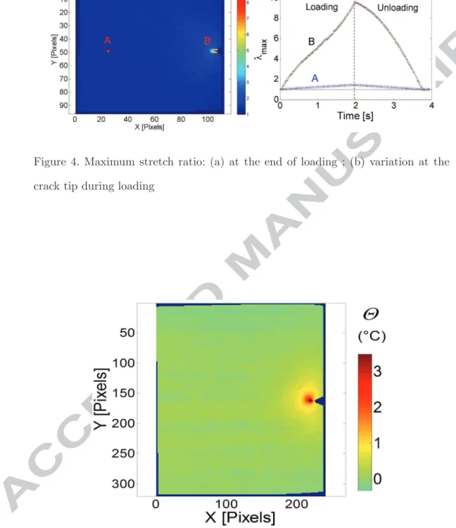
Figure 4(a) presents a map of the maximum stretch ratio at the end of loading. The maximum stretch ratio is quite homogeneous over all the specimen surface except in the vicinity of the crack tip zone. Figure 4(b) presents the variation in the maximum stretch ratio at two different points. Point A is located out of the zone of influence of the crack and point B is located in the crack tip zone, where its value is the highest. Three comments can be made from this figure:
• the variation in the maximum stretch ratio at point A corresponds to the global stretch ratio variation;
• at point B, the maximum stretch ratio at the end of loading is equal to 9.5. It must be noted that even if this value depends on the data processing (chosen correlation parameters), it is much higher than the stretch ratio at failure in a homogeneous PS test (approximately 5). In the latter case, failure occurs from the lowest mechanical strength zone. This high stretch ratio value corresponds to the limit of chain extensibility. Indeed, by fitting the stress-strain curves obtained with constitutive models to reflect limiting chain extensibility [26], the maximum chain extensibility corresponds to a stretch ratio of about 10;
• at point B, the curve shape between loading and unloading is not symmet-rical.
4.1.2 Calorimetric analysis
Electronic version only: details on maximum stretch ratio evolution can be found in the video presented in Appendix B.
Figure 5 presents the map of temperature changes for the maximum global stretch ratio (λ = 1.5). The maximum value is equal to about 3.5◦C. It is
located at a distance of about 8 pixels from the crack tip, corresponding to 0.5 mm.
The zone of high temperature changes is more or less circular. The shape of this zone is influenced by the heat diffusion. Consequently, this approach does not enable us to localize accurately the heat source. It is therefore more relevant to examine the maps of heat sources deduced from the temperature changes instead of the temperature change field itself.
Figure 6 presents the heat source distribution for the maximum stretch ratio. A strong localization is observed very close to the crack tip. The heat source localization corresponds to a zone of about 7 pixels (horizontal profile A-A) by 5 pixels (vertical profile B-B), corresponding to about 0.44×0.32 mm2
. Outside this zone, the heat sources are negligible compared to the maximum heat source, which is equal to 56◦C/s. Figure 7 presents the variation in time
of the heat source in the crack tip vicinity at point B (see Fig.4), where the heat source value is the highest. Some comments can be made for the loading phase of the first cycle:
• the heat source first slightly increases. This is in agreement with heat sources due to entropic coupling [27], with possible additional small mechanical dissipation;
• the heat source then strongly increases. It can be split into two contribu-tions: that of the entropic coupling and that of the mechanical dissipation, if any. The former quantity is positive for a positive strain rate. The latter is always positive as it is related to mechanical irreversibilities, such as damage or viscosity. It is not possible to distinguish the mechanical dissipation in the total heat source without modeling or considering the whole mechanical cycle.
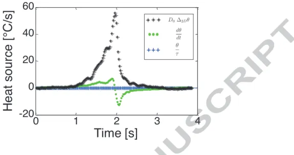
The results obtained for the unloading phase show that the heat source remains positive during unloading: first it strongly decreases, then progressively returns to zero. The entropic coupling heat source is expected to be negative since the strain rate is negative. This means that, during unloading, there is the production of a (positive) mechanical dissipation whose amplitude is higher than the entropic coupling term. This result is significant because it shows that the crack tip is a zone which always produces heat during cyclic tests, favoring the self-heating of this zone. Consequently, this zone is probably more affected by phenomena such as thermo-oxidation. To the best of the authors’ knowledge, this result has never been reported in the literature. Finally, it is interesting to compare the relative weights of the three terms of the left-hand side of Eq. 3. Figure 8 shows the variation in time of dθ/dt, θ/τ and −D0∆2Dθ
during the first cycle:
• it can be noted that the term θ/τ is negligible. This means that the heat given to the ambient air by convection is negligible over the tests performed; • it can be observed that the main part of the total heat source is contained
in the conduction term −D0∆2Dθ;
hand side of Eq. 3 shows that the diffusion term cannot be neglected in the processing of temperature fields with a strong localization.
4.2 Analysis of the second and the tenth cycles
Stress softening is classically considered to occur during the first ten cycles [7]. Moreover, the most important loss in stiffness is obtained between the first and second cycles [7]. This is the reason why the second and the tenth cycles are also analyzed in the present study.
Figure 9 presents the variation in the maximum stretch ratio λmaxat the crack
tip for the first, second, and tenth cycles. Several comments can be made from this figure:
• at any time, the maximum stretch ratio at the crack tip for the first cycle is inferior or equal to that of the second and tenth cycles;
• the loading curve shape of cycle 1 is different from the loadings of cycles 2 and 10. However, the unloading curve shapes are similar for all three. It can be noted that for cycles 2 and 10, the curve is symmetrical between loading and unloading. This property is not observed for cycle 1. This can be explained by the fact that stress softening mainly occurs during the first cycle;
• the curves of cycles 2 and 10 are very similar except for the highest stretch ratio levels.
As stress softening can be thought to modify the map of the loading states in the zone of influence of the crack, Figure 10 gives the map of the biaxiality ratio b for the tenth cycle. It is observed that the size of the zone of influence
of the crack has not changed between the first and tenth cycles (compare with Figure 3c). It can be also seen that near the crack tip, the values of the biaxiality ratio remain the same between the first and tenth cycles. Moreover, a high level of mechanical dissipation was observed during the first cycle. The question is to know whether this is also observed during cycles 2 and 10. Figure 11 presents the variation of the heat sources at the crack tip for the first, second, and tenth cycles. Several comments can be drawn from this figure:
• for cycles 1, 2 and 10 the heat sources during unloading remain positive and small. As explained in section 4.1.2, this is certainly due to (positive) mechanical dissipation due to viscosity which is added to the (negative) thermoelastic coupling heat source;
• the heat sources during loading decrease with the number of cycles. This is explained by the fact that the mechanical dissipation decreases with the number of cycles. This is in agreement with a progressive accommodation of the material at the crack tip. It should be noted that it is quite difficult to distinguish the relative contributions of the effects of viscosity, stress softening and possibly crack propagation (even if it is very low in the present case) to the heat source during loading.
As a remark, the thermomechanical response at the crack tip strongly dif-fers from that of less stretched zones. Indeed, in zones at the centre of the specimen, where the maximum stretch ratio attained is equal to 1.5, the heat sources are negative during unloading, meaning that the effects of mechanical dissipation (positive) during unloading are not superior to those of entropic coupling (negative). This is shown in Figure 12a. In this figure the thermoe-lastic inversion is clearly observed. Due to the low level of stretch ratio and
strain rate, the effects of the variation in internal energy and entropy are of the same order of magnitude. This leads to a low temperature variation over time, which can be observed in Figure 12b, contrary to the temperature variation over time at the crack tip, (see Figure 12c).
5 Conclusion
In the present study, full kinematic and thermal field measurements were per-formed at the crack tip of a carbon black filled SBR specimen during cyclic loading. For several cycles in the range of the Mullins effect, both kinematic and calorimetric analyses were carried out. First, the results obtained in terms of kinematic analysis have shown that at the end of loading high stretch ra-tios levels can be observed at the crack tip, which are much higher than the measured stretch ratio at failure in a homogeneous test. This was explained by the high extensibility of chains. The distribution of the strain states and the strain levels have been mapped for the different mechanical cycles applied. Second, the results obtained in terms of heat sources can be summarized as follows: (i) the zone of the highest heat source values is much more confined than the zone of the highest temperature due to heat conduction; (ii) contrary to the case of the homogeneous loading observed at the centre of the specimen, the heat sources during unloading remain positive and small at the crack tip. This is due to the fact that, for these loading conditions and material for-mulation, the mechanical dissipation has the same order of magnitude as the thermoelastic coupling. Finally, even though the material only produces heat (no detectable heat absorption) at the crack tip, the heat production decreases with the number of cycles, which is in good agreement with the fact that the
material is progressively accommodated. These initial results are promising to improve constitutive modeling of rubber and motivate further work in the field of the fatigue and aging of the crack tip zone.
6 Acknowledgments
The authors would like to thank the ”Manufacture Fran¸caise des pneumatiques Michelin” for supporting this study. We also thank J. Caillard for the fruitful discussions.
Appendix A: supplementary data
The online version of this article contains a video showing the evolution of maximum stretch ratio evolution during the first cycle.
Appendix B: supplementary data
The online version of this article contains a video showing the evolution of the heat sources evolution during the first cycle.
References
[1] R. S. Rivlin and A. G. Thomas. Rupture of rubber. i. characteristic energy for tearing. J. Polym. Sci., 10:291–318, 1953.
[2] A. A. Griffith. The phenomena of rupture and flow in solids. Phil. Trans. R. Soc. B , A, 221:163–198, 1921.
[3] E. H. Andrews. Generalized theory of fracture mechanics. J. Mater. Sci., 9(6):887–894, 1974.
[4] E. H. Andrews and Y Fukahori. Generalized fracture mechanics .3. pre-diction of fracture energies in highly extensible solids. J. Mater. Sci., 12(7):1307–1319, 1977.
[5] J.-B. Le Cam. A review of the challenges and limitations of full-field measurements applied to large heterogeneous deformations of rubbers. Strain, 48:174–188, 2012.
[6] E. Toussaint, X. Balandraud, J.-B. Le Cam, and M. Gr´ediac. Combining displacement, strain, temperature and heat source fields to investigate the thermomechanical response of an elastomeric specimen subjected to large deformations. Polym. Test., 31:916–925, 2012.
[7] J. Diani, B. Fayolle, and P. Gilormini. A review on the mullins effect. Eur. Polym. J., 45:601–612, 2009.
[8] M. A. Sutton, W. J. Wolters, W. H. Peters, W. F. Ranson, and S. R. McNeill. Determination of displacements using an improved digital cor-relation method. Image Vision Comput., 1:133–139, 1983.
[9] P. Vacher, S. Dumoulin, F. Morestin, and S. Mguil-Touchal. Bidimen-sional strain measurement using digital images. P. I. Mech. Eng. C-J. Mec., 8:811–817, 1999.
[10] T. Pottier, M.-P. Moutrille, J.-B. Le Cam, X. Balandraud, and M. Gr´ediac. Study on the use of motion compensation technique to de-termine heat sources. application to large deformations on cracked rubber specimens. Exp. Mech., 49:561–574, 2009.
of a new motion compensation technique in infrared stress measurement based on digital image correlation method. Nihon Kikai Gakkai Ronbun-shu, A Hen/Trans. Jap. Soc. Mech. Eng., 72:1853–1859, 2006.
[12] P. Schlosser. Infuence of thermal and mechanical aspects on deformation behaviour of NiTi alloys. Phd thesis, universit´e Joseph Fourier, Grenoble, 2008.
[13] A. Chrysochoos, B. Wattrisse, J.-M. Muracciole, and Y. El Kaim. Fields of stored energy associated with localized necking of steel. J. Mech. Mater. Struct., 4:245–262, 2009.
[14] D. Delpueyo, M. Gr´ediac, X. Balandraud, and C. Badulescu. Investiga-tion of martensitic microstructures in a monocrystalline Cu-Al-Be shape memory alloy with the grid method and infrared thermography. Mech. Mater., 45:34–51, 2012.
[15] A. Chrysochoos and H. Louche. An infrared image processing to analyse the calorific effects accompanying strain localisation. Int. J. Eng. Sci., 38:1759–1788, 2000.
[16] H. Louche and A. Chrysochoos. Thermal and dissipative effects accom-panying l¨uders band propagation. Mater. Sci. Eng. A-Struct., 307:15–22, 2001.
[17] J. R. Samaca Martinez, J.-B. Le Cam, X. Balandraud, E. Toussaint, and J. Caillard. Filler effects on the thermomechanical response of stretched rubbers. Polym. Test., 32:835 – 841, 2013.
[18] B. Berthel, A. Chrysochoos, B. Wattrisse, and A. Galtier. Infrared image processing for the calorimetric analysis of fatigue phenomena. Exp. Mech., 48:79–90, 2008.
[19] A.E. Morabito, A. Chrysochoos, V. Dattoma, and U. Galietti. Analysis of heat sources accompanying the fatigue of 2024 T3 aluminium alloys.
Int. J. Fatigue, 29:977–984, 2007.
[20] J.G. Harris and Y.-M. Chiang. Nonuniformity correction of infrared im-age sequences using the constant-statistics constraint. IEEE T. Imim-age Process., 8:1148–1161, 1999.
[21] S. N. Torres and M. M. Hayat. Kalman filtering for adaptive nonuni-formity correction in infrared focal-plane arrays. J. Opt. Soc. Am. A, 20:470–480, 2003.
[22] C. Badulescu, M. Gr´ediac, H. Haddadi, J.D. Mathias, X. Balandraud, and H.S. Tran. Applying the grid method and infrared thermography to investigate plastic deformation in aluminiummulticrystal. Mech. Mater., 43:36–53, 2011.
[23] X. Balandraud, E. Ernst, and E. Soos. Influence of the thermomechanical coupling on the propagation of a phase change front. C. R. Acad. Sci., Ser. II B, 329:621–626, 2001.
[24] D. Delpueyo, X. Balandraud, and M. Gr´ediac. Heat source reconstruc-tion from noisy temperature fields using an optimised derivative gaussian filter. Infrared Phys. Techn., 60:312–322, 2013.
[25] A. Stormy. Butterworth-Heinemann ltd, 2011.
[26] A. N. Gent. A new constitutive relation for rubber. Rubber Chem. Tech-nol., 69(1):59–61, 1996.
[27] J. R. Samaca Martinez, J.-B. Le Cam, X. Balandraud, E. Toussaint, and J. Caillard. Thermal and calorimetric effects accompanying the deforma-tion of natural rubber. part 2: quantitative calorimetric analysis. Polymer, 54:2727 – 2736, 2013.
List of Tables
Table 1 Formulation in phr Ingredient Styrene-Butadiene rubber (SBR) 100 Carbon black 50 Antioxidant 6PPD 1.9 Stearic acid 2
Zinc oxide ZnO 2.5
Accelerator CBS 1.6
List of Figures
1 Specimen geometry: (a) front view; (b) side view. 29
2 Experimental device 30
3 Characterization of the strain states at the end of the first
loading 31
4 Maximum stretch ratio: (a) at the end of loading ; (b) variation
at the crack tip during loading 32
5 Map of temperature changes θ for the maximum global stretch
ratio. 32
6 Map of heat sources S/ρ0CE for the maximum global stretch
ratio. The Maximum value of the heat source is equal to 56°C/s, but the color scale is limited to 20°C/s for a better
visualization of the heat source localization 33
7 Heat source versus time at the crack tip for the first cycle. 33
8 Variation over time of the three terms of the left-hand side of
the heat diffusion equation. 34
9 Variation in the maximum stretch ratio at the crack tip during
cycles 1, 2 and 10 34
10 Map of the biaxiality ratio at the specimen surface at the end
11 Variation over time of the heat sources at the crack tip during
cycles 1, 2 and 10. 35
12 Variation over time of heat sources and temperature variations
(a) strain states in the plane of the two invariants (I1, I2)
(b) cartography of strain states using the two invari-ants I1 andI2 at the specimen surface
(c) cartography of strain states using the biaxiality ratio at the specimen surface
Figure 4. Maximum stretch ratio: (a) at the end of loading ; (b) variation at the crack tip during loading
Figure 6. Map of heat sources S/ρ0CE for the maximum global stretch ratio. The
Maximum value of the heat source is equal to 56°C/s, but the color scale is limited to 20°C/s for a better visualization of the heat source localization
0
1
2
3
4
-20
0
20
40
60
Time [s]
H
e
a
t
so
u
rce
[
°C
/s]
− D0∆2Dθ dθ dtFigure 8. Variation over time of the three terms of the left-hand side of the heat diffusion equation.
Figure 9. Variation in the maximum stretch ratio at the crack tip during cycles 1, 2 and 10
Figure 10. Map of the biaxiality ratio at the specimen surface at the end of the tenth loading
Figure 11. Variation over time of the heat sources at the crack tip during cycles 1, 2 and 10.
(a) Variation over time of the heat sources at the specimen center during cycles 1, 2 and 10
(b) Variation over time of the temperature varia-tions at the specimen center during cycles 1, 2 and 10
(c) Variation over time of the temperature variations at the crack tip during cycles 1, 2 and 10
• We investigate the thermomechanical response of cracked CB-filled SBR specimens
• We couple full thermal and kinematic field measurements during cyclic loadings
• The zone of influence of the crack and the maximum stretch ratio level are measured
• We show that mechanical dissipation is high and confined to the crack tip
• Mechanical dissipation decreases with the number of cycles