Design and development of a network architecture for a chemical sensor network

Design and Development of a Network

Architecture for a Chemical Sensor

Network

by

Jimmy Cheung

Submitted to the Department of Electrical Engineering and Computer Science in Partial Fulfillment of the Requirements for the Degrees of

Bachelor of Science in Electrical Engineering and Computer Science and Master of Engineering in Electrical Engineering and Computer Science

MASACHUSMrTS INSTUE.

at the Massachusetts Institute of Technology OF TECHNOLOGY

May 19, 2005 JAt

-O8

2005

Copyright 2005 Jimmy Cheung. All rights reserved.

LIBRARIES

distribute publicly paper and electronic copies of this thesis and to grant others the right to do so.

Author

D rtment Electrical Engi.eLring and Computer Science May 19, 2005 Certified by

ptf6fe'ssr Harold F. Hemond

T;psis Supervisor Accepted by______

'Arthur C. Smith Chairman, Department Committee on Graduate Theses

Design and Development of a Network

Architecture for a Chemical Sensor

Network

by

Jimmy Cheung

Submitted to the Department of Electrical Engineering and Computer Science May 19, 2005

In Partial Fulfillment of the Requirements for the Degrees of Bachelor of Science in Electrical Engineering and Computer Science and Master of Engineering in Electrical Engineering and Computer Science

Abstract

A real-time continuous chemical sensor network can obtain detailed data to analyze the

dynamic behavior of water systems such as a lake. The behaviors of interest to us in Upper Mystic Lake are the effects of stratification on methane water chemistry and the results of water mixing between layers. To monitor the water chemistry, a network of three buoys is populated with various sensors. This paper covers the design implementation of the network architecture for transmitting sensor data between buoys and a shore station. The buoys' sensors and construction are also included.

Thesis Supervisor: Harold F. Hemond

TABLE OF CONTENTS

1

2.2 HARDW ARE CONVENTIONS ... 8

2.3 POW ER SUPPLY ... 9

3 SO FTW A RE PLA TFO RM ... 12

3.1 Buoy SYSTEM TS - LINUX ... 12

3.2 M O O S PLATFORM ... 12

3.3 SHORE STATION DEBIAN LINUX PLATFORM ... 13

4 NETW O R K SO FTW A R E ... 14

4.1 N ETW ORK SUMMARY ... 14

4.2 PNETW ORKTx ... 16

4.2.1 Process Sum m ary ... 16

4.2.2 Configuration ... 17

4.2.3 Process Details ... 17

4.2.4 Future W ork ... 18

4.3 PNETw ORKRx ... 19

4.3.1 Process Sum m ary ... 19

4.3.2 Configuration ... 19

4.3.3 Process Details ... 19

4.3.4 Future W ork ... 21

4.4 PNETW ORKHUB ... 21

4.4.1 Process Sum m ary ... 21

4.4.2 Configuration ... 22

4.4.3 Process Details ... 22

4.4.4 Future W ork ... 23

4.5 PNETLOGGER ... 24

4.5.1 Process Sum m ary ... 24

4.5.2 Configuration ... 24 4.5.3 Process Details ... 25 4.5.4 Future W ork ... 26 4.6 RESULTS ... 26 5 INSTRUM EN TS ... 28 5.1 XEMics G PS ... 28 5. 1. 1 Hardware ... 28 5.1.2 Software ... 29 5.1.3 Configuration ... 30 5.1.4 Future W ork ... 30 5.2 HYDROLAB M INISONDE ... 31 5.2.1 Hardware ... 31 5.2.2 Software ... 31 5.2.3 Configuration ... 32 5.2.4 Future W ork ... 32 5.3 THERMISTOR C HAIN ... 33 5.3.1 Hardware ... 33 5.3.2 Software ... 36 5.3.4 Configuration ... 37

5.3.3 Future W ork... 37 5.4 A couSTic M ODEM ... 37 5.4.1 Hardware ... 37 5.4.2 Software... 39 5.4.3 Configuration... 40 5.5 M ETS SENSOR ... 40 5.5.1 Hardware ... 40 5.5.2 Future W ork... 41 6 PH Y SICA L C O N STR U C TIO N ... 41 7 CO N CLU SIO N ... 43 8 A CK N O W LED G EM EN TS ... 43

APPENDIX A - SOFTWARE QUICK GUIDE... 44

APPENDIX B - BUOY COMPACT FLASH SETUP... 46

APPENDIX C - TS-5500 JUMPER CONNECTIONS ... 51

APPENDIX D - DESKTOP/SHORE STATION DEBIAN LINUX SETUP... 53

APPENDIX E - MOOS SOFTWARE DEVELOPMENT ... 56

APPENDIX G - TS-5500 SOFTWARE DEVELOPMENT... 61

1 Introduction

1.1 Scientific Motivation

The buoy network and sensor system is part of a National Science Foundation

(NSF) funded project to study heterogeneous fluxes in lakes. These heterogeneous fluxes

arise from the thermal stratification in lakes caused by the seasonal warming and cooling. The temperature differences cause the stratified layers of water to have very different chemical compositions. The lower colder layer or hypolimnion tends to have a lower dissolve oxygen but higher methane content than the upper warmer layer also known as the epilimnion. If the two chemically distinct layers mix, there would be interesting chemical reactions that may occur. These heterogeneous fluxes can be caused by various events such as winds cooling the surface causing a pocket of cold water to sink into the hypolimnion, also known as a plunging thermal[5].

These plunging thermals and other heterogeneous fluxes are difficult to quantify due to their transient nature. Environmental studies generally regularly sample data by hand which does not have a very high resolution over time. To catch these transient events, a real-time sensor network is needed. These interesting water chemistry dynamics motivate the development of a two part sensor network to provide real-time water chemistry data. The buoy's network of sensors is one part that provides high resolution water chemistry data at certain water columns chosen throughout a lake. The second part consists of an autonomous underwater vehicle (AUV) outfitted with various sensors including a mobile mass spectrometer from the project NEREUS. Through interpolation of data and through dynamic sampling by the AUV, the system's sensor range will encompass much of the lake and possibly provide enough data to analyze the

effects of heterogeneous fluxes. The entire network is represented in Figure 1.1[5], taken from the NSF proposal and is drawn by Heidi Nepf.

Z --

t-wind

Z - ~ ..- ~ weather station

arrayI arrav2 arrav3 network node

upwelling T(z)

'Nsurface pLAgn

lay er thffnals

NEEU 2 -rich

Figure 1.1 Graphical conception of entire network system. [5]

This paper concentrates on the development and implementation of the buoy sensor network and hopes to serve as a manual for the upkeep and future development of additional features. Additional information on NEREUS and the AUV can be found in Rich Camili and Adam Champy's thesis and SeaGrant's documentation, respectively

1.2 Implementation

The implementation of the buoy sensor network required the interaction and help of SeaGrant, Professor Harold Hemond, Adam Champy, and Terence Donoghue. Prof. Hemond and SeaGrant provided a lot of guidance on the project and Champy and Donoghue help fabricate the electrical and mechanical aspects, respectively. Donoghue built most of the hardware, flotation, and moorings necessary to provide a stable platform for a water tight Rose enclosure which houses the embedded computer system. The computer system is powered by a power board, custom designed by Champy. Additional sensors were attached via water proof cables and bulkhead connectors which feed into the

rose enclosure and to various ports on the embedded computer. Most of the hardware and wiring is already complete. The current software runs in Linux and can retrieve data from most of the sensors, log the data, and send it wirelessly to a shore station. The rest of the paper presents the details of each components and the appendix goes into further details about the steps needed to reproduce the buoy system hardware and software.

2 Hardware Platform

2.1 Embedded Comruter

Figure 2.1 TS-5500 from Technologic Systems mounted on a PVC plate.

The computer system we use came from Technologic Systems [1] (http://www.embeddedx86.com). My predecessor, Joseph Wong, made the choice of using the TS-5500 (Figure 2.1), a PC 104 form factor embedded computer. The system board is fairly rich in features and has a decently supported Linux operating system. The

specifications listed on their website are in Figure 2.2.

PC compatible Single Board Computer with 133 MHz AMD 5x86 processor. . 32-64 MB SDRAM . 10/100 Ethernet . 2 USB ports . PCMCIA socket

. Compact Flash socket . 3 COM ports

. 38 DIO

. PC/104 expansion bus . 2 MB Flash drive . Optional A/D converter

Figure 2.2 Specifications[1] for the TS-5500.

Two of the systems have 64MB of SDRAM memory while the original has 32MB. I opted for more memory since it will help in improving performance for the multi-process configuration. A TS-SER4 card is also stacked on each TS-5500 adding 4 extra

COM/serial ports. In addition, the PC104 system has a PCMCIA 802.1 lb Orinoco card to enable network connectivity.

The TS-5500 runs off a Linux operating system that is loaded onto a compact flash card. For the setup of the compact flash card, Technologic Systems supplies the data files and instructions on its website. (Beware the instructions and files are updated and changed fairly frequently) Appendix B covers the detailed instructions necessary for creating a compact flash for the computer system.

2.2 Hardware Conventions

In the implementation of the hardware, there are certain conventions that were chosen in order to make things easier to remember and systematic. One of these conventions is the association of COM ports to certain sensors. Although the association

is easily adjustable, it is preferable to maintain a consistent mapping to avoid any confusion in configuration files and wiring.

Port Sensor/Instrument Baud Rate

DIO 1 Thermistor Chain N/A

COMI -/dev/ttySO GPS 9600 8N1

COM2 -/dev/ttyS 1 Console Terminal (fixed) 115200 8N1(Linux 3.07+)

9600 8N1 (Bios)

COM3 - /dev/ttyS2 Hydrolab 19200 8N1

COM4 -/dev/ttyS3 Acoustic Modem 19200 8N1

COM5 -/dev/ttyS4 METS 9600 8N1

COM6 -/dev/ttyS5 (unused)

COM7 -/dev/ttyS6 (unused)

Figure 2.3 Port to Sensor Mapping with baud rates for each sensor. Note the differences between the windows COM# reference to Linux's /dev/ttyS# reference to the same port. COM4 and COM5 are on the T-SER4 board and are labeled as COMA and COMB, respectively.

Although some systems may be missing certain sensors the association should conform to the mapping in Figure 2.3. There are two more available serial ports so the convention can accommodate two additional serial devices before requiring a rearrangement of the mapping. Also it is important to note that the TS-SER4 board requires the COM4, IRQ2, and IRQ4 pins to be jumped in order for the intuitive sequential ordering of the additional COM ports. (In the new 3.07 version of TS-Linux, these settings are simply reiterated in /etc/init.d/tsserial ) Please see Appendix C for additional jumper settings for the TS-5500 and TS-SER4.

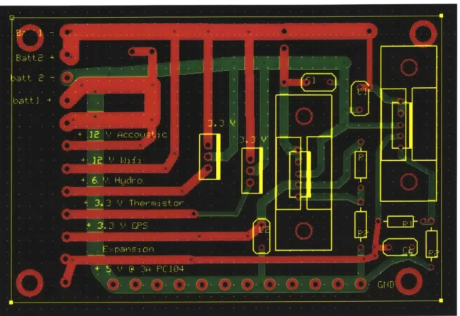
r 2.4 Circuit Layout of Power Control Board. The image is best viewed in color or electronically to see traces and their connections.

Figure 2.6 Picture of the Power Control Board.

The power control board shown in Figure 2.4 is designed by Adam Champy, a fellow Masters in Engineering student and my colleague on the project. Please see Appendix H for more information regarding components of the power board. Its main components are an adjustable 5A regulator at -5.2-5.3V and a 3.3V regulator which supplies the necessary voltages for many of the sensors and devices. The battery inputs are also wired together to create a 12 volt source. The voltage supplies the respective devices in Figure 2.5.

Power Devices Total Draw

Source

3.3 V Xemics GPS (20mA), Thermistor Chain ~ 20-21mA Board (22 uA[3])

5.2-5.3V TS-5500(900 mA[3]) -900mA

6.OV Acoustic Modem(2-3.4A on Tx), Hydrolab(36 -2-3.5A (variable on transmit

(Battery) mA - 85 mA[3]) frequency)

12V Hyperlink 2.4Ghz 1 Watt Amplifier 1.25A Peak Tx and 0.14A Peak I Rx [4] (variable on Tx)

Figure 2.5 Table of Power Sources and devices connected.

The ports on the board are connected using terminal strips. The design of the board allowed stacking of additional PCB boards like the Thermistor and GPS board to save space on the PVC plate mounted on the Rose enclosure's lid.

Most of the wiring was done with solid or stranded 22 gauge hookup wire. The PC104 and acoustic modems require larger current draws so their connections are 18 gauge. The connection of the power board to the battery uses two sets of 18 gauge wire

(18 gauge can supply -2.3 amps[2] so two sets are used to supply the 1 amp draw from

the TS-5500 and 2-3 amp draw from the Acoustic Modem) with two pin Molex connectors to allow easy connections. The single two pin male Molex plug from the power board powers the upper +6 volts for the 12V supply. Care should be taken to plug

in the two sets of Molex connectors first then the single two pin Molex connector and unplug in reverse order to prevent any potentially adverse circuit paths.

3 Software Platform

3.1 Buoy system TS - Linux

The Linux systems on the TS-5500 on the buoys are very similar to a minimal Debian Linux configuration, but are actually based on Mandrake. The operating system has been customized by Technologic Systems for the TS-5500 and their other embedded systems. The customizations help make certain that the software will correctly support the hardware and has recently added configuration automations. It features a couple of useful programs such as: SSH (Secure SHell) server, Apache web server, Minicom (Linux Terminal program), and Vi (text editor). For future work and convenience an Emacs text editor would be preferable to Vi, but it would have to be manually installed.

The SSH server uses the SSH2 protocol to allow remote logins to perform any administrative tasks over a network connection. This allows access to the system without connecting to the buoy console terminal using the physical connection; however, if something should interfere with the normal startup of the SSH server the terminal connection is the failsafe in managing the system's software. Improper startups have been caused by improper shutdowns which result in a corrupted file system. Correction of file system anomalies require user interaction and a wired terminal connection since the SSH server cannot start. Appendix B describes in detail the locations of necessary configuration files.

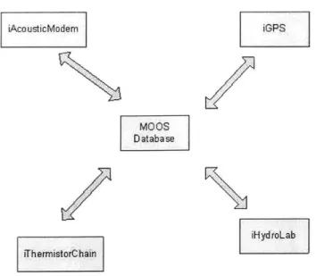
UE 'J iAcousticModem iGPS MOOS Database iHydroLab lThermistorChain

Figure 3.1 Example MOOS data flow diagram.

The Mission Oriented Operating Suite (MOOS) was designed and implemented

by Paul Newman at MIT SeaGrant.[8] SeaGrant uses the software platform to run autonomous underwater vehicles (AUV). MOOS sets up every sensor or instrument as a separate process and has a database called MOOSDB to act as a bulletin board between processes as illustrated in Figure 3.1. This configuration allows for modularity and provides fault tolerance. By using MOOS, the system also gains many built-in or available functionalities and compatibility with SeaGrant's AUV systems. For a description of MOOS configuration please see Appendix F. For information on software development for MOOS see Appendix E.

3.3 Shore Station Debian Linux Platform

The shore station is currently configured as a Debian Linux workstation. Debian Linux seems to be the best choice due to its reputation for rock-solid stability and ease of adding additional features through the apt-get command. In the author's experience, the system has only crashed a handful of times over the course of a year and being on

consistently. The stability comes at the cost of difficult initial setup and slow incorporation of advanced features. Another advantage is that many of the configuration settings are similar to the TS - Linux on the buoy. Evaluations of Red Hat's Fedora Core

3 (the best alternative and a popular up and coming Linux distribution) indicate lack of

stability in writing to compact flash cards and reaffirms the decision to go with Debian Linux. Appendix D goes into detail how to install Debian Linux on the specific Dell

systems in lab, but can be applied to most hardware.

4 Network Software

BUOY1

1

iHydrolab

2

HYDROLABPH

pNetworkHub TWORKRX_MSG MOOSDB NETWORKTXMSG pNetLogger

3

pNetworkRx pNetworkTx

5

TCP/IP Wireles Tranmission TCP/IP Wireles Tranmission

Shore

6

pNetworkTx io,~, pNetworkRx

NETWORKRX_MSG

BUYl_HYDROLAB_PH MOOSDB BUOY1_HYDROLABPH pNetworkHub

pLogger

8

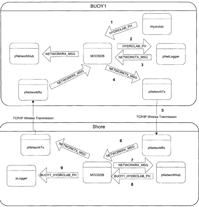
Figure 4.1 Data Flow Diagram. The sequential numbers represent the data flow from the Hydrolab sensor on Buoy 1 to the pLogger process on the shore station..

The network architecture for our network of buoy systems is shown in Figure 4.1. The buoy systems use four MOOS processes to communicate data in between nodes in the network. In step 1 of Figure 4.1, the iHydrolab process reports the pH value from the

sensor to the variable HYDROLABPH. The variable HYDROLABPH is watched by pNetLogger which takes in the data and packages the data for network transport (adds necessary headers and appends BUOY1 to the MOOS variable name) and sends the data

packet or message to NETWORKTXMSG. The pNetworkTx process reads off the new message, NETWORKTXMSG, and sends it over the wireless link using TCP/IP socket connections to the shore station.

On the shore station side, the pNetworkRx process receives the data and stores it to NETWORKRXMSG in step 6. The new network message NETWORKRXMSG is then parsed by pNetworkHub and the MOOS variable in the message is posted to the MOOSDB. The logging process pLogger watches for the resulting variable and value and stores it to a file in the final step. The transmission of commands from shore to a buoy uses the path and processes as described above. The following sections go into detail regarding the individual processes and their configurations.

4.2 pNetworkTx

4.2.1 Process Summary

The pNetworkTx process is responsible for all outgoing communications from a

MOOS community or system. It mainly subscribes to the NETWORKTXMSG MOOS

variable and attempts to send the message to the destination indicated in the message. Upon receiving a message it looks up the IP address of the intended destination and opens a TCP/IP socket to transmit the message over port 5000 on the destination system. Once transmitted the process completes and awaits the next NETWORKTXMSG message.

The outgoing link handler pNetworkTx is chosen to be independent of the incoming link pNetworkRx to increase modularity and reduce complexity in the code. The drawback is an increase in number of socket connections, which the Linux system and hardware are estimated to be able to handle at least twenty sockets. These should be

able to handle 5-10 buoys within each system's extended 802.1 lb range and is definitely sufficient for our current network of three buoys, one shore station, and the AUV.

4.2.2 Configuration

Each MOOS Process has a configuration block that is required for it to run. It also has important configuration settings. For pNetworkTx the configuration block is shown in Figure 4.2. ProcessConfig = pNetworkTx { AppTick = 1 CommsTick = 4 Port = 5000 NodeName = BUOY1 MOOSNode = 192.168.0.1 SHORE MOOSNode = 192.168.0.2 BUOY1 MOOSNode = 192.168.0.3 BUOY2 MOOSNode = 192.168.0.4 , BUOY3 MOOSNode = 192.168.0.5 AUV }

Figure 4.2 pNetworkTx MOOS configuration block.

The important settings are Port, NodeName, and MOOSNode. The Port setting determines the port on the destination to make a TCP/IP socket connection. NodeName is not used currently but is nice to set and may be in future revisions. MOOSNode supplies an association between NodeNames and their respective IP addresses. These IP's are arbitrarily chosen and manually set, but they should agree with the entries in /etc/hosts file and in the /etc/pcmcia/network.opts file on each buoy. Adding additional nodes requires adding a new line with the corresponding information.

4.2.3 Process Details

pNetworkTx is a single threaded process that relies on incoming MOOS messages from the NETWORKTXMSG variable to trigger outgoing communications. The key code block is in Figure 4.3.

bool CMOOSNetworkTx::SendData(string node,char* data, int length) {

mNameToSocketMap[node] = new XPCTcpSocket(mlDataPort); string IPAddress = m_MOOSNameToIPMap[node];

if (IPAddress.size() ==O) {

MOOSTrace("CMOOSNetworkTx::SendData - NC - Node not in Config file\n"); break; } try { //opens socket

m_NameToSocketMap [node] ->vConnect (IPAddress.c -str()); MOOSTrace ("Socket connect Success %s:%s:%d\n",

node. c_str () , IPAddress. c_str () , milDataPort) ;

//one second wait, may not be necessary MOOSPause(1000);

//send data

nSent = mNameToSocketMap [node] ->iSendMessage (data, length);

MOOSTrace("MOOSNetworkTx: SendData): sent %d %s\n", nSent, data);

//close connection

m_NameToSocketMap.erase(node); return true;

}

Figure 4.3 pNetworkTx's SendData function.

The MOOS class XPCTcpSocket provides most of the abstraction for working with TCP sockets. If one looks through the code completely, one would notice that the process was originally meant to keep connections open as much as possible; however, upon a disconnection a sent message would reconnect but the message would not get delivered. Therefore the code is changed to open and close the connection on each transmission to guarantee delivery and simplify the process.

4.2.4 Future Work

There are a few additional features that would be helpful for the pNetworkTx. On failures to send, the pNetworkTx should either post back to the MOOSDB with the failed message or queue it for future transmissions. The queue would add a fair amount of code

and complexity to the system but would prevent data loss due to a downed link. Also, if the link is down for a long time, the queue may grow too large and require storage to a file. The process can resume communications when the link has been restored.

4.3 pNetworkRx

4.3.1 Process Summary

The multi-threaded MOOS process pNetworkRx manages all incoming connections from port 5000 and posts any received messages to NETWORKRXMSG. One thread handles the job of listening to new connections while the other checks on current connections. In theory the two jobs could be combined but the author was not successful at doing both in one thread. The code is heavily borrowed from the MOOSCommServer class and that class also uses multiple threads. The handling of multiple concurrent connections makes this process the most complex of the four network processes.

4.3.2 Configuration

The MOOS configuration of pNetworkRx requires only a port number to listen as shown in Figure 4.4 ProcessConfig = pNetworkRx { AppTick = 1 CommsTick = 4 Port = 5000 }

Figure 4.4 pNetworkRx's MOOS configuration block.

The first of two threads is the ListenLoop thread. As its name implies, the thread creates an XPCTcpSocket on port 5000 and listens until it gets a connection. Once a client connects, the thread creates a new XPCTcpSocket for the connection and places it into a client socket list. The important code snippets are shown in Figure 4.5. Once on the client socket list, the ServerLoop thread will check for any new messages from that connection.

bool CMOOSNetworkRx::ListenLoop() char sClientName[200];

//listen for new connection m_pListenSocket->vListen (;

//found new connection create new socket for it

XPCTcpSocket * pNewSocket = m-pListenSocket->Accept(sClientName); MOOSTrace ("Adding new Network Connection from %s\n", sClientName);

//lock socket list for writing

m_SocketListLock.Lock(;

//add new connection's file descriptor(Fd) to socket list

m_ClientSocketNameList [pNewSocket->iGetSocketFd() ]= sClientName; m_SocketListLock.UnLock();

Figure 4.5 pNetworkRx's ListenLoop thread.

The second thread, ServerLoop, runs the C++ function select to check multiple sockets for data. To use select, one must give it a set of file descriptors (an integer representing a socket connection). The key parts of the code are shown in Figure 4.6. Once data is available, the select function returns with another file descriptor set of the sockets with data. The ServerLoop thread then checks the list of sockets with the

information from select and reads the data accordingly. Afterwards, the process posts the data to NETWORKRXMSG and loops back into running select again.

bool CMOOSNetworkRx::ServerLoop()

{

//setup file descriptor sets and arguments for select

FD_ZERO(&fdset);

SOCKETLIST::iterator p,q;

//rotate list..

m_ClientSocketList.pushjfront(rm_ClientSocketList. back();

m_ClientSocketList.pop-back();

for(p = m_ClientSocketList.begin() ;p!=mClientSocketList.end() ;p++)

{ FDSET((*p)->iGetSocketFd(), &fdset); } m_SocketListLock.UnLock(; timeout.tvsec = 1; timeout.tvusec = 0;

//running select to watch for data

int iSelectRet = select(mnMaxSocketFD + 1, &fdset, NULL, NULL, &timeout);

//something to read: m_SocketListLock.Lock(;

for(p m_ClientSocketList. begin() ;p! =mClientSocketList. end() ;p++)

{

//member pointer to reference a socket with data m_pFocusSocket = *p;

//check if socket is in the set returned by select

if (FDISSET(m-pFocusSocket->iGetSocketFd(), &fdset) 0)

{

//something to do read: if(!ProcessClient() Figure 4.6 pNetworkRx's ServerLoop thread.

4.3.4 Future Work

The code for pNetworkRx is fairly robust and is based on the MOOSCommServer, which has been working very well in MOOS for a while. This process does very little message processing to consolidate most of the network logic into pNetworkHub. At the moment the pNetworkRx process requires no additional features or revisions.

4.4 pNetworkHub

4.4.1 Process Summary

The pNetworkRx and pNetworkTx handles most of the low level socket layer transmissions details between MOOS communities. pNetworkRx places all received

messages into NETWORKRXMSG to be parsed and processed by pNetworkHub. pNetworkHub currently only reads in messages sent by pNetLogger, but its logic can easily be extended to read new message types and perform other functions. For the messages from pNetLogger, it parses out the initial network headers and extracts the

MOOS variable name, value, time, and data type. Once extracted, the data is posted to

the MOOSDB to make it available for other processes. In the case of Figure 4.1, the HYDROLABPH data from Buoyl is made available in the variable BUOY 1_HYDROLABPH. The process works similarly for all other data and MOOS variables.

4.4.2 Configuration

pNetworkHub only requires the most basic configuration as shown in Figure 4.7. ProcessConfig = pNetworkHub

{

AppTick = 1

CommsTick = 4 }

Figure 4.7 pNetworkRx's MOOS configuration block.

4.4.3 Process Details

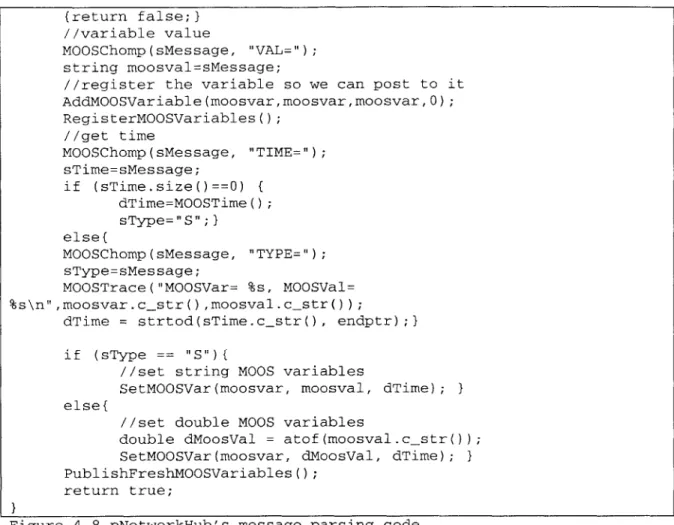
The pNetworkHub process is simple since it only involves string parsing and code to carry out necessary commands or functions for the messages received. Most changes and addition of logic will occur in the code block in Figure 4.8.

bool CMOOSNetworkHub::ProcessMessage(char* data, int length) {

//remove DEST entry

MOOSChomp (sMessage, "DEST="); string sMessageChomp = sMessage;

string sNodeName=MOOSChomp(sMessage, ","); //variable name

MOOSChomp (sMessage, "VAR=");

string moosvar=MOOSChomp(sMessage, ",1");

{return false;} //variable value

MOOSChomp(sMessage, "VAL=" ); string moosval=sMessage;

//register the variable so we can post to it AddMOOSVariable (moosvar,moosvar,moosvar, 0); RegisterMOOSVariables(); //get time MOOSChomp(sMessage, "TIME="); sTime=sMessage; if (sTime.size()==0) { dTime=MOOSTime(); sType="S";} else{ MOOSChomp(sMessage, "TYPE="); sType=sMes sage; MOOSTrace("MOOSVar= %s, MOOSVal= %s\n",moosvar.cstr(,moosval.cstr());

dTime = strtod(sTime.cstr(, endptr);}

if (sType == "S")(

//set string MOOS variables

SetMOOSVar(moosvar, moosval, dTime); else{

//set double MOOS variables

double dMoosVal = atof(moosval.c_str());

SetMOOSVar(moosvar, dMoosVal, dTime); PublishFreshMOOSVariables();

return true;

}

Figure 4.8 pNetworkHub's message parsing code.

4.4.4 Future Work

Looking at the code block in Figure 4.8, the linear parsing of the text file does make it awkward to add additional message types and arguments. The parsing should be changed to a switch type of architecture similar to the way MOOS configuration files are read. These changes have not been made as of the writing of this paper but may be completed soon after.

The code for pNetworkHub will need change for each additional feature or command. It supplies the network interface between MOOS communities. It can also accommodate a message passing or multi-hop architecture in case of broken links and

indirect paths are available. As of now it only contains the base functionality of posting

MOOS variables from other MOOS communities' pNetLogger processes.

4.5 pNetLogger

4.5.1 Process Summary

pNetLogger is the network analog of the file logger pLogger. The process pNetLogger subscribes to specified MOOS variables and posts any new variable data at a

specified rate to NETWORKTXMSG for transport to the shore station. Although it currently directly posts to NETWORKTXMSG, eventually it will deliver data to pNetworkHub first to allow for multi-hop capabilities.

4.5.2 Configuration

The configuration is nearly exactly the same for pLogger for consistency reasons. The general format can be seen in Figure 4.9. An important new setting is the Prefix which is how the same data from two different buoys can be differentiated on the shore station. The prefix is appended to any MOOS variable names sent to the shore station. Adding new MOOS variables to be logged over the network require adding a new line into the configuration file.

ProcessConfig = pNetLogger

{

//over loading basic params...

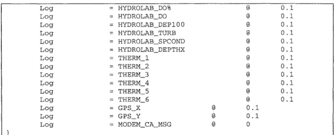
AppTick = 10.0 CommsTick = 10.0 Prefix = BUOY1 SyncLog = true @ 0.2 // Log = Test @ 0.1 // Log = DEPTHDEPTH @ 0.1 / Log = NETWORKTXMSG @ 0.1 Log = HYDROLABTIME @ 0.1 Log = HYDROLABTEMP @ 0.1 Log = HYDROLABPH @ 0.1

Log = HYDROLABDO% @ 0.1 Log = HYDROLABDO @ 0.1 Log = HYDROLABDEP100 @ 0.1 Log = HYDROLABTURB @ 0.1 Log = HYDROLABSPCOND @ 0.1 Log = HYDROLABDEPTHX @ 0.1 Log = THERM_1 @ 0.1 Log = THERM_2 @ 0.1 Log = THERM_3 @ 0.1 Log = THERM_4 @ 0.1 Log = THERM_5 @ 0.1 Log = THERM_6 @ 0.1 Log = GPSX @ 0.1 Log = GPSY @ 0.1 Log = MODEMCAMSG @ 0 }

Figure 4.9 pNetLogger's MOOS configuration block.

4.5.3 Process Details

In the code for pNetLogger shown in Figure 4.10, the ParseNewMail function contains most of the key components. In MOOS, all variable updates are sent as a

MOOSMSGLIST. ParseNewMail takes this list and checks for variables matching what

it is logging and then extracts the necessary data. The data is then packaged into a string message and posted to NETWORKTXMSG.

bool CMOOSNetLogger: :ParseNewMail (MOOSMSG_LIST &NewMail)

{

MOOSMSG_LIST::iterator q; //iterate through all mail

for(q = NewMail.begin();q!=NewMail.end();q++) {

CMOOSMsg & rMsg = *q;

//check if we are logging this variable

iff (mMOOSVars. find(rMsg. -m_sKey) !=mMOOSVars.end())

{

string Msg; string sType;

double dTime = rMsg.GetTimeo;

if (rMsg.IsDataType(MOOSDOUBLE)) { sType="D";}

else{

sType="S";

//convert double value to string ostrstream os;

os.setf(ios::left);

os<<setw(12)<<dTime<<ends;

string sTime = os.str(; os.rdbuf()->freeze(0);

Msg = "DEST=SHORE,VAR=" + msPrefixName + "_"+

Msg.GetKey() + ",VAL=" + rMsg.GetAsString() + ",TIME=" + sTime +

",TYPE=" + sType;

//Post new NETWORKTXMSG to MOOSDB

SetMOOSVar ( "NETWORKTX_MSG", Msg, MOOSTime ());

PublishFreshMOOSVariables(); }

}

return true;

Figure 4.10 pNetLogger's ParseNewMail function.

4.5.4 Future Work

pNetLogger works well in its current state and does not need much further modification. The only foreseeable change is to pass messages through to pNetworkHub for multi-hop functionality instead of directly to the pNetworkTx.

4.6 Results

The network software was tested in lab numerous times and has been able to achieve transmission of data from the buoy systems to a system setup as the shore station. On May 10, 2005 two buoys were set out on Upper Mystic Lake with a laptop serving as the shore station. The network software and architecture were able to transmit thermistor chain data from both buoys and post it onto the MOOSDB of the shore station. The test proves the functionality of the current network. Although one of the buoys also had a Hydrolab, it was accidentally not configured to run in the configuration process. The

GPS data was not available since the driver was not developed for the Xemics device.

However the thermistor chain data was sufficient to test the data flow of the network software. The logs (Figure 4.11) from the laptop, which acted as a simulated shore station, demonstrate the ability of the network software to transmit sensor data across the wireless link. Figure 4.12 is a graph of some thermistor data collected from logs and

6989.891 6989.891 6989.891 6989.891 6989.891 6989.891 6989.891 6989.891 -33010.109 -33010.109 -33010.109 -33010.109 -33010.109 -33010.109

BUOY2_MODEMCAMSG pNetworkHub $CATXF BUOY2_THERMI pNetworkHub 11.625 BUOY2_THERM_2 pNetworkHub 11.375 BUOY2_THERM_3 pNetworkHub 10.375 BUOY2_THERM_4 pNetworkHub 3.875 BUOY2_THERM_5 pNetworkHub 3.625 BUOY2_THERM_6 pNetworkHub 3.875

BUOY2_MODEMCAMSG pNetworkHub $CAREV

BUOY1_THERM_2 pNetworkHub 11.875 BUOY1_THERM_3 pNetworkHub 12.125 BUOYlTHERM_4 pNetworkHub 11.875 BUOY1_THERM_5 pNetworkHub 11.875 BUOY1_THERM_6 pNetworkHub -16.125 BUOY1 THERM_1 pNetworkHub 15.875

Figure 4.11 pLogger Files from the simulated shore station.

5 Instruments

5.1 Xemics GPS

5.1.1 Hardware

Figure 5.1 Xemics RGPSM002 GPS device

The Xemics GPS device is a close to stamp size GPS device with an attached stamp size antenna. The actual model number is RGPSM002 and the data sheet can be found on the web [6]. In Figure 5.1, one can see the tiny size of this device. The hardware interface is a 16 pos flat flex cable with .5mm pitch. The vertical surface mount (SMT) connectors are Molex PN: 52559-1692 and they were ordered from www.mouser.com. (52746-1690 and 52745-1690 would also work, but the vertical mounts are easier to solder since the SMT mounts are spread out).

... ....-

~ -... .-

Figure 5.2 Xemics RGPSM002 GPS device Circuit Board

The pins of the SMT mount of interest are 1 (GROUND, 3 (VCC 3.3V), 5 (Serial RXA), and 7 (Serial TXA). The GPS runs off a 3.3V power source and partly due to this reason the voltage output from the device cannot drive a RS232 port. Therefore, an RS232 driver chip (Part. No. ST3232E) uses capacitors to help increase the voltage levels so that the embedded computer can communicate with the device. The wiring and

specifications for the RS232 driver chip is simple and can be found in its datasheet and in Appendix H. Figure 5.2 shows the circuitry involved to power and communication with the GPS device. The top lines in the figure are power and ground. The 10 pin headers on the right allow a straight through ribbon connection to the PC104's COMI port.

5.1.2 Software

$GPGSA,A,2,26,21,29,,,,,,,,,,4.30,4.18,1.00*043,4.18,00033,M,-033,M,,*69C3,M,-03 $GPGGA,183745.0,4221.74205,N,07105.36675,W,1,04,1.95,00033,M,-033,M,,*6563,M,-03

The software for the Xemics GPS simply takes in textual input from the serial port and parses the text for the coordinate information. Like most GPS devices, it follows the NMEA message format and posts coordinate information in the $GPGGA message as shown in Figure 5.3. The latitude and longitude information are highlighted in the $GPGGA message. The $GPGSA message is also useful in determining when the

GPS system is tracking since it may take a while to get a lock. The bolded 2 indicates the

fix information. As long as the output shows a 2 or 3 in the $GPGSA message the GPS has a valid fix.

5.1.3 Configuration ProcessConfig = iXemicsGPS AppTick = 8 CommsTick = 4 Port = /dev/ttySO BaudRate = 9600 Streaming = true

Figure 5.4 iXemicsGPS's MOOS configuration block.

The MOOS driver for the Xemics GPS device is similar to other GPS devices and the required configuration is the same too. The port must be set to the correct COM port and the baud rate should be 9600 with Streaming set to true. The settings can be seen in Figure 5.4.

5.1.4 Future Work

GPS devices are fairly simple to integrate and although the GPS is not currently

working at the time of writing this thesis, it should be fully operational before the summer. The only other issue with the GPS is that it may not always be able to get a lock on its coordinates although it usually does. If it becomes a problem, then it should be investigated more thoroughly.

5.2 Hydrolab Minisonde

Figure 5.13 Hydrolab Minisonde 4a.

Joseph Wong's thesis [3] covers much of the work regarding the Hydrolab Minisonde (Figure 5.13). The hardware has not changed much since his time on the project. The Hydrolab can accept a large range of voltages, but we will be running it off the 6V battery to use the voltage meter on the Hydrolab to gauge the battery life for the system. The wiring is summarized in Figure 5.5.

Female MiniSonde Bulkhead DB-9 Female, 9-Pin, D-Sub

Bulkhead 1 4,6, Power (Viewed from the front)

-1 2 5, Ground 5 4 3 2 1

d

1 . . .

3 40 4 2 . ...

5 8 9 8 7 6

6 9

Figure 5.5 Wiring pinout for Hydrolab. Consolidated from Joseph Wong's Thesis [3].

5.2.2 Software

Initially, Joseph Wong had been able only to use the terminal emulation method of retrieving data from the Hydrolab instrument. This made timing issues complicated and required a lot of message parsing of the output. After speaking with a technical support person at Hydrolab, it was learned that the instrument has a TTY mode which allows streaming of data without a console. To get into TTY mode, connect a console

with settings 19200 8N1 and then go to Setup>Display >TTY. This should reset the device and have it start streaming data in order. To exit TTY mode, press spacebar to pause then

Q

002638 24.28 38.8 1.97 -1.31 7.48 477 002639 24.28 38.8 1.97 -1.31 7.48 477

HIM?: H n/a

Time Temp DO% SpCond Dep25 pH ORP

HHMIMSS

sC

Figure 5.6 Example Hydrolab Output with header command sent.

5.2.3 Configuration ProcessConfig = iHydrolab { AppTick = 10 CommsTick = 10 Port = /dev/ttyS2 BaudRate = 19200 Streaming = true }

Figure 5.7 iHydrolab's MOOS configuration block.

The MOOS driver for the Hydrolab instrument is similar to the GPS device. The port must be set to the correct COM port and the baud rate should be 9600 with

Streaming set to true. The settings can be seen in Figure 5.7.

5.2.4 Future Work

The current software retrieves header information automatically; however, to be consistent with MOOS and due to Rob Damus' suggestions the header information

should be set in the MOOS configuration file by hand. Although this adds extra work on the user, the settings are more transparent and can be renamed. Knowing the names of the variables beforehand will help in configuring pLogger and pNetLogger.

5.3 Thermistor Chain

Figure 5.7 Last thermistor probe of a thermistor chain. The thermistor chain consists of a series of thermistor probes like the one in Figure 5.8. There are two sets of 6 probe chains and one set of 5 probes. Because the software by Joseph Wong was hard-coded for 6 chains, the non-existent chain reports a

-16 value. The probes detect temperature by using a temperature sensitive resistive

element. All thermistor probes share a common ground wired to pin 2 of the SeaCon connector on the thermistor chain. (Not intuitive but that's the way it is setup). Each remaining pin correlates sequentially to the probes on the chain.( pin 1,3,4,5,6,7 goes to probe 1,2,3,4,5,6)

Figure 5.8 Combined Tnermistor upS PCb oara.

Because we were missing the third thermistor board, the PCB board was recreated and combined with the GPS board to save costs and space, shown in Figure 5.8. The new PCB board moves away from the RJ45 jacks used on the old board and uses header and ribbon cable connections to the DIO port. The spaces on the upper left quadrant are for a terminal strip to connect to the thermistor chain bulkhead. However due to an incorrect assumption about the original RJ45 wiring and inconsistencies in the documentation the wiring was reversed. To fix the reversal, the order of cables had to be changed on the terminal strip (Figure 5.9), the ribbon cable needed to swap the necessary pins (Figure

5.10), a connection had to be jumpered, and a trace disconnected (both in Figure 5.11).

Figure 5.9 New Order of Wire connections to Thermistor Bulkhead.

Figure 5.10 Rewiring of 16pin ribbon cable. Rearranged wires 1<->13, 3<->9, 5<->14, 7<->8.

Figure 5.11 Thermistor Board modifications.

Once all the changes were made, the thermistors worked with Joseph's original software. The tiny chip on the PCB board is a MAX6682, which converts thermistor resistances to digital values. The large chip is a low voltage analog multiplexer MAX4638 and is used to select a specific thermistor probe line. The wiring diagram can be obtained from Figure 5.8 or the PCB file. Alternatively the information is also available in the appropriate datasheets or Joseph Wong's thesis.

5.3.2 Software

The MOOS driver for ThermistorChain was written by Joseph Wong [3] and the details on it can be found in his thesis. In summary, it sends certain bits over the DIO to set the multiplexer and then reads the resulting digitized value from the thermistor chip.

These values are then placed into the MOOS variables THERM_1, THERM_2, THERM_3 and so on.

5.3.4 Configuration ProcessConfig = iThermistorChain { AppTick = 1 CommsTick = 1 CollectionTick = 0.05 }

Figure 5.12 iThermistor's MOOS configuration block. The configuration is fairly typical and allows the data collection frequency can be changed.

5.3.3 Future Work

One of the project's goals is to create sensor networks that can self calibrate. The thermistor chain is one sensor that is easy to configure and also prone to drift. Therefore, future work should make the MOOS driver able to calibrate the thermistor chain to more accurate instruments like the Hydrolab or the AUV. There should also be some research into making the thermistor chain have higher resolution in temperature readings since it currently has a resolution of 0.125 degrees. This possibly involves choosing a better thermistor chip to convert analog resistance or voltage values to digital. One could also change the thermistor driver to account for different length thermistor chains but it may be easier to just ignore the extra data.

5.4 Acoustic Modem

Figure 5.14. Acoustic modem bottle profile view

Figure 5.15. Acoustic Modem Bottle top view

For underwater communication and navigation with the AUV, each buoy has an acoustic modem supplied by the Woods-Hole Oceanographic Institute (WHOI). The electronics of the modem are housed in an aluminum bottle shown in Figure 5.14. Two connections can be made to the bottle shown in Figure 5.15. The bottle connects to a 6 pin cable which leads to power and a RS232 interface. The 3 pin connector leads to the transducer element. The buoys use a high frequency transducer in order to prevent noise pollution in the lake environment. These transducers tend to have some directionality in their transmission so the strongback assembly in Figure 5.16 is necessary to keep the transducer vertical.

Figure 5.16. Transducer and Strongback assembly.

For the cabling from the bottle to the transducer, the wiring diagram is available from WHOI (Drawing No. 234003-SCH). Since the cable end changed after the cables were ordered, the correct pigtails had to be soldered and potted onto the original cables. The buoy to bottle cable is a pass through going from a MIL9 type to a 7 pin CCP type connector. The wiring diagrams and information can be found in Appendix H.

For the initial deployment, the micromodems connect straight off the 6V battery supply. From the tests during the summer and fall of 2004, Lee Freitag estimated that the optimal power range for the modems should be near 6V. Due these tests, WHOI

modified the modems to support variable voltages from 6-24V. The current draw is

highly variable and can peak up to 3+ amps during transmit.

5.4.2 Software

Rob Damus developed the original acoustic modem driver and is currently adding additional functionality to allow for data transfer and long base line (LBL) navigation. For our purposes, the current driver does not have much functionality other than basic transmit and receive commands. Once the driver is updated, the data will most likely be posted to some MOOS variable so that any other process such as pNetLogger can read it and transfer the data to the shore station.

---5.4.3 Configuration ProcessConfig = iAcousticModem { Type = WHOIV2.5 AppTick = 8 CommsTick = 10 Port = /dev/ttyS3 BaudRate = 19200 Verbose = true TxEvery = 8 ModemAddress = 2 }

Figure 5.12 iAcousticModem's MOOS configuration block. Due to the new MOOSInstrument Family architecture the

configuration also requires a device type.

5.5 METS Sensor

Figure 5.13 Photograph of the METS sensor.

The METS sensor made by Capsum (Figure 5.13) will enable the buoy to obtain methane concentration information. The author has very limited experience with the

METS sensor since it arrived near the end of this semester. Because the buoy systems

had to be placed out in the field early on, the wiring for the METS sensor was completed before any development of software. The wiring diagram is similar to the acoustic modem and is available in the manual for the METS sensor and in Appendix H. The sensor requires at least 9V so the buoy will supply it with 12V off the same supply as the wireless amplifier, which is two 6V batteries in series.

5.5.2 Future Work

The METS sensor is fairly different in its data acquisition from the other sensors on the buoy. It does not stream data so the system will have to periodically send command strings to retrieve data from the device. A MOOS driver will have to be developed for the METS to enable integration into the buoy system.

6 Physical Construction

Terence Donoghue is the main contact for any information regarding the physical construction of the buoys and mounting hardware. The author's contribution to the physical construction mainly involved the physical wiring and layout of Rose enclosure. During the development of the buoy systems, the embedded computer and most of the component ended up mounted on the lid of the Rose enclosure to enable easy access and efficient use of space. The batteries remained in the main compartment and attach to the power supply board via the 2 pin Molex connectors. One can see the improvement of the original setup in Figure 6.1 to the new layout in Figure 6.2.

Most of the devices are mounted on a PVC plate with through holes. Most of the mounted hardware has lock washers and standoffs to protect it from coming loose or developing a short circuit. The wireless amplifier currently sticks to the PVC plate using Velcro, but may need a more robust solution in the future. The PVC plate connects to the lid through threaded bolts and threaded holes in the fiberglass. The wire harness feeds through twist-locks and wire ties across the hinge to prevent tension and chafing from the opening and closing of the lid. Once the wires reach the main compartment they split and connect to the bulkhead connectors or terminate in Molex connectors for the batteries.

Figure 6.1 Original Rose Enclosure Layout with most components removed.

Figure 6.2 Current Layout of Rose Enclosure with all components.

7 Conclusion

Although the main thesis of this paper involves the development of a network architecture for this chemical sensor network, it involved the construction of the buoy system and integration of instruments in order to test the network layer of the system. The field trials and laboratory experiments show the network layer to be working properly. With the network component realized, the project goes on step further to achieving the goal of an automated high resolution and dynamic chemical sensor network. The next step is to add additional features to various components of the system

and add multi-hop functionality to the wireless link.

8 Acknowledgements

I would first like to Thank Professor Harold Hemond for supervising me on this

thesis project. His guidance has helped me on various aspects of the project. I would like to also thank Terence Donoghue for helping during the field tests, constructing the buoys and assisting with the internal layout. His assistance and company has been invaluable. Thanks go to Adam Champy and Amy Mueller as well for helping out on other parts of the project and for being wonderful colleagues. Our research group is also appreciates the assistance and collaboration from SeaGrant and WHOI in making this project possible. Finally we thank National Science Foundation for funding this exciting project that has provided many insights into sensor network development.

Appendix A - Software Quick guide

If everything is automated, one should just plug in the CF card, plug power to the main

power board (double two-pin Molex connectors) and then power the 12 sources (single two-pin Molex connector)

The current configuration runs automated scripts by adding commands to the tsserial script in /etc/init.d/tsserial. At the end of the tsserial script all serial devices should be configured so we can start the program by adding the line:

/home/MOOSBin/runMOOS &

The ampersand allows the program to run on its own thread so it does not block the startup of later scripts.

The automated MOOS startup script is in the file /home/MOOSBin/runMOOS #! /bin/sh

# starts pAntler with configuration NetworkParsons.moos export PATH=$PATH:/home/MOOSBin

/home/MOOSBin/pAntler /home/MOOSBin/network.moos

Contents of /home/MOOSBin/runMOOS. The script runs the first command export to set a path to the executables then runs the pAntler program to run all MOOS processes in the network.moos file.

Manually Running MOOS

1. To manually run MOOS, one must start the system and log in via terminal (using

minicom, hyperterminal or securecrt using the baud rate 115200 8N1 --- 9600 8N1 was

original used for pre 3.07 version of TS -Linux and is still used for the BIOS and DOS portions) or SSH (ssh2 for current system., sshl for pre TS -Linux 3.07)

SSH Commands

ssh 192.168.0.2 (password is redhat)

2. Once logged in, type the following commands: cd /home/MOOSBin/

export PATH=$PATH:/home/MOOSBin/ pAntler network.moos

The setup basically reiterates the automated commands from the startup script. The export path command is important in giving Linux a global link to find executables and libraries.

Preconfigured Settings

Appendix B - Buoy Compact Flash Setup

This guide goes through the creation of a fresh compact flash setup for the buoys. This is mostly based on the compact flash setup instructions by Technologic Systems

(http://www.embeddedx86.com/linux/htm] docs/new cf method.html ).[1] The key steps are to set the image, transfer files to the two partitions, and then transfer setting files over. Each file setting will also be described in the end.

1. Obtain all necessary files from www.embeddedx86.com or from the hemond locker

http://web.mit.edu/hemond/Buoy/*.

Easiest way is to scp the files over using the command: [one line] scp -r

username@athena.dialup.mit.edu:/afs/athena.mit.edu/org/h/he mond/Buoy/* /mnt/

This command should retrieve all the necessary files and output it to the /mnt/ directory. 2. Plug in CF card reader and insert 512 MB Sandisk Ultra II CF cards. (CF card reader

support should be covered in Linux desktop setup in Appendix D.

3. Copy disk image to CF card.

cd /mnt/flashfiles/

bunzip2 TS-base-512.cf.bz2

dd if=TS-base-512.cf of=/dev/sda bs=1M

The second line decompresses the image file to the 512MB image. The third dd

command copies the file image stored in TS-base-512.cf and writes it to the file /dev/sda (Linux tries to represent everything as file and so the CF card appears as the file

/dev/sda). The bs=1M is new and is important for making different CF cards more consistent.

(NOTE: The dd command is useful to backup images of a working CF card as well. Just

reverse the input file(if) and output file(of) to save a CF image to a file. You may only want to backup the /dev/sda2 partition since you cannot mount the /dev/sda without a CF card.)

4. Unplug CF card when step 3 is complete. Plug it back in to allow mounting of new partitions.

5. Create and mount CF card partitions 1 and 2. Partition 1(/dev/sdal) is the DOS

partition which stores the kernel image and loads the Linux file system on the ext2 file system on Partition 2(/dev/sda2).

cd /mnt/ mkdir cfl

mkdir cf2

mount /dev/sdal cf1 mount /dev/sda2 cf2

6. Copy all base linux files over to CF card

cd /mnt/flashfiles/ tar -C /mnt/cf2 -xvzf TS-3.07a.tar.gz tar -xvzf TS-FAT-3.07a.tgz cp -dp ./TSLinuxFAT/* /mnt/cf1 tar -xvzf kernel-486-2.4.23-2.5tgz cp -dp /kernel-486-2.4.23-2.5/bzImage /mnt/cfl tar xvzf modules-kernel-486-2.4.23-2.5.tgz cp -dpR ./2.4.23-2.5 /mnt/cf2/lib/modules

7. Copy MOOSBin executables over to /home/MOOSBin

d /mnt/

cp -r MOOSBin /mnt/cf2/home/

8. Copy preconfigured setting files for buoyl over to CF card. (change to buoy 2 and

buoy 3 as necessary) cd /mnt/ cp -r buoy1/* /mnt/cf2/ 9. Umount cf cards umount /mnt/cf 1 umount/mnt/cf2 Setting Explanations

The directory buoyl-buoy3 collect together all the various little files and modifications

necessary to run the software or configure the network. Each file and its relevance is described below.

Startup settings 1. /etc/init.d/tsserial

We make changes to the tsserial script for two reasons. First the serial port setup is close but not exactly correct for the TS-5500 with its on board 3 COM ports. Therefore we need to change it to setup the TS-SER4 COM A to COM 4. We do that making the changes below:

mknod -m 666 /dev/ttyS3 c 4 67

mknod -m 600 /dev/ttyS4 c 4 68

mknod -m 600 /dev/ttyS5 c 4 69 mknod -m 600 /dev/ttyS6 c 4 70

if [ $? -eq 122 ];then

echo Found a TS-SER4

setserial -v /dev/ttyS3 port Ox2e8 autoirq autoconfig Afourport setserial -v /dev/ttyS4 port Ox3a8 auto_irq autoconfig ^fourport setserial -v /dev/ttyS5 port Ox2a8 autoirq autoconfig ^fourport setserial -v /dev/ttyS6 port Ox3aO autoirq autoconfig Afourport

fi

/home/MOOSBin/runMOOS &

At the end of the file we also add the command to startup the MOOS script. This is a good spot since all the serial devices will have been setup.

Network Files 2. /etc/hosts

The hosts file provides Domain Name Service resolution of IP addresses to a string or name. The current hosts file looks like:

127.0.0.1 localhost.localdomain localhost 192.168.0.5 sub sub 192.168.0.6 laptop2.mit.edu laptop2 192.168.0.7 laptop3.mit.edu laptop3 192.168.0.1 shore shore 192.168.0.2 buoyl buoyl 192.168.0.3 buoy2 buoy2 192.168.0.4 buoy3 buoy3

The hosts file is usually not important if you know by memory the IP addresses and serves as a convenience; however, in MOOS a hosts file entry is REQUIRED for any

MOOS Process to connect to the MOOSDB. Therefore if we want to use MOOSScope to

peek at the MOOSDB we need our IP address in that host file or else it throws a error. The network software works independent of this.

3. /etc/pcmcia/network.opts

This network.opts file configures the network parameters for the wireless card or ethi in linux. The important settings are:

IFPORT=""

# Use BOOTP (via /sbin/bootpc, or /sbin/pump)? [y/n]

BOOTP="n"

# Use DHCP (via /sbin/dhcpcd, /sbin/dhclient, or /sbin/pump)? [y/n]

DHCP="n"

# If you need to explicitly specify a hostname for DHCP requests

DHCPHOSTNAME=""

# Host's IP address, netmask, network address, broadcast address IPADDR="192.168.0.2"

NETMASK="255 .255.255.0" NETWORK="192 .168.0.0" BROADCAST="192.168.0.255"

# Gateway address for static routing GATEWAY="192.168.0.1"

We basically turn off DHCP and assign a static IP address. You can look at the /etc/hosts file to see which buoy should have what address. The convention so far is 192.168.0.1 is

the shore station, 192.168.0.2 is Buoyl, 192.168.0.3 is Buoy2, and 192.168.0.4 is Buoy3. The remaining settings are the same for all buoys.

4. /etc/pcmcia/wireless.opts

The wireless.opts file sets a few configuration parameters for the purely wireless aspects of the network. Our systems use a Lucent Wavelan IEEE card also known as the original Orinoco. For this card, we want the ESSID set to Parsons and Mode set to ad-hoc. One can also set the security KEY in this file to provide WEP encryption in the wireless link. Each network node must have the same KEY to able to communicate.

# Lucent Wavelan IEEE (+ Orinoco, RoamAbout and ELSA)

# Note : wvlancs driver only, and version 1.0.4+ for encryption

support

*,*,*,00:60:1D:*I*,*,*,00:02:2D:*)

INFO="Wavelan IEEE example (Lucent default settings)" ESSID=" Parsons" MODE= "Ad-hoc" # RATE="auto" # KEY="s:secul" Libararies 5. /lib/libpthread.so.0 6. /usr/lib/libstdc++-libc6.2-2.so.3

These are two additional library files necessary for the MOOS software to run. The programs just will complain that they are missing if it is not found.

(NOTE: If the MOOS software complains of missing other libraries, please check that

you have compiled correctly in Appendix E. This errors happens when the software is compiled in the wrong environment (hence different version of the library files

If you are sure that you require the new libraries then copy them over from the TS-Dev cd image used in the compilation in Appendix E)

Utilities

7. /home/minicom

Minicom is a terminal program that is useful for peeking at specific COM ports to see if the sensors are outputting data. It is not necessary for running the system.

8. /home/setserial

Setserial is there for legacy reasons to be able to configure specific serial ports. It may be included in the default file system in 3.07. Not necessary.

MOOSFiles

9. /home/MOOSBin/network.moos

This is the main configuration file for the MOOS software. Details are available in Appendix F

10. /home/MOOSBin/runMOOS

This is a simple script that runs the export PATH command runs pAntler on the network.moos file.

#! /bin/sh

# starts pAntler with configuration NetworkParsons.moos

export PATH=$PATH:/home/MOOSBin