HAL Id: inserm-00747058
https://www.hal.inserm.fr/inserm-00747058
Submitted on 7 Nov 2012
HAL is a multi-disciplinary open access
archive for the deposit and dissemination of
sci-entific research documents, whether they are
pub-lished or not. The documents may come from
teaching and research institutions in France or
abroad, or from public or private research centers.
L’archive ouverte pluridisciplinaire HAL, est
destinée au dépôt et à la diffusion de documents
scientifiques de niveau recherche, publiés ou non,
émanant des établissements d’enseignement et de
recherche français ou étrangers, des laboratoires
publics ou privés.
intracardiac electrograms using a dynamic time delay
artificial neural network.
Fabienne Porée, Amar Kachenoura, Guy Carrault, Renzo Dal Molin, Philippe
Mabo, Alfredo Hernandez
To cite this version:
Fabienne Porée, Amar Kachenoura, Guy Carrault, Renzo Dal Molin, Philippe Mabo, et al.. Surface
electrocardiogram reconstruction from intracardiac electrograms using a dynamic time delay artificial
neural network.. IEEE Transactions on Biomedical Engineering, Institute of Electrical and Electronics
Engineers, 2013, 60 (1), pp.106-14. �10.1109/TBME.2012.2225428�. �inserm-00747058�
Surface Electrocardiogram Reconstruction from
Intracardiac Electrograms Using a Dynamic Time
Delay Artificial Neural Network
Fabienne Porée, Amar Kachenoura, Guy Carrault, Renzo Dal Molin, Philippe Mabo and Alfredo I. Hernández
Abstract—The study proposes a method to facilitate the remote follow-up of patients suffering from cardiac pathologies and treated with an implantable device, by synthesizing a 12-lead sur-face ECG from the intracardiac electrograms (EGM) recorded by the device. Two methods (direct and indirect), based on dynamic Time Delay artificial Neural Networks (TDNN) are proposed and compared with classical linear approaches. The direct method aims to estimate 12 different transfer functions between the EGM and each surface ECG signal. The indirect method is based on a preliminary orthogonalization phase of the available EGM and ECG signals, and the application of the TDNN between these orthogonalized signals, using only three transfer functions. These methods are evaluated on a dataset issued from 15 patients. Correlation coefficients calculated between the synthesized and the real ECG show that the proposed TDNN methods represent an efficient way to synthesize 12-lead ECG, from two or four EGM and perform better than the linear ones. We also evaluate the results as a function of the EGM configuration. Results are also supported by the comparison of extracted features and a qualitative analysis performed by a cardiologist.
Index Terms—Implantable device, ECG reconstruction, Intrac-ardiac electrogram, Time delay neural networks.
I. INTRODUCTION
T
HE number of patients treated with Implantable Cardiac Devices (ICD) has strongly increased over the past 10 years. According to the American Heart Association [1], an estimated 111 000 defibrillator and 358 000 pacemaker implant procedures were performed for patients in the United States in 2007. These patients require regular in-hospital visits to follow-up the patient’s response to the therapy, to monitor whether the ICD is working optimally and, eventually, to modify the pacing parameters. More recently, wireless remote monitoring of ICD has become a priority for all major ICD constructors, in order to perform this follow-up more frequently, avoiding hospital visits and reducing costs. In both cases, the surface electrocardiogram (ECG) is necessary, since it is the main signal used by the cardiologist for the analysis of the cardiac electrical activity. However, the cardiac electrical activity acquired from the ICD, called electrograms (EGM), are collected by electrodes placed on the endocardium and/orF. Porée, A. Kachenoura, G. Carrault, P. Mabo and A.I. Hernández are with INSERM, U1099, Rennes, F-35000, France, and also with the Université de Rennes 1, LTSI, Rennes, F-35000, France
P. Mabo is also with CHU Rennes, Service de Cardiologie et Maladies Vasculaires, Rennes, F-35000, France, and with the CIC-IT 804, INSERM, Rennes, F-35000, France.
R. Dal Molin is with Sorin CRM, Clamart, France. Manuscript received xx.
the epicardium and show different morphologies than those of the surface ECG. The synthesis, or reconstruction, of the surface ECG from a set of EGM is thus of first importance in this context.
This challenging problem has been dealt by a number of studies [2]–[9]. From a methodological point of view, they can be categorized according to the method used to estimate the Transfer Function (TF) between EGM and ECG: i) linear filtering methods based upon Recursive Least Squares (RLS) estimation or by processing the data in blocks [2]–[4], [9], ii) single, fixed-dipole modeling algorithms [8], [9], and iii) non linear filtering methods [2], [5], [6].
Concerning the linear approach, several works have been proposed in the literature. In [2], each surface QRS com-plex was synthesized using a direct single-input single-output scheme. We showed in this work that the direct ECG synthesis depends strongly on the chosen EGM and that a multivariate approach would be of benefit. In this sense, we proposed in [3], [4] an indirect method to estimate the linear TF between three-dimensional (3D) representations of cardiac activity [10], namely the signal EGM3D, obtained from the orthogonaliza-tion of EGM signals and the signal ECG3D derived through the orthogonalization of ECG signals.
In the same line of the above-mentioned methods, Menden-hall et al presented recently the use of a multivariate linear TF [8], [9]. Although the performance of these linear meth-ods is satisfactory, especially for patients with surface ECG containing only one beat morphology, some improvements are still needed. In fact, in a real application, noise, artifacts and the natural evolution of the pathology may influence the relationship, over time, between the EGM and the ECG. Thus stochastic and non linear phenomena crop up, and time series dynamics cannot be robustly described using classical linear filtering.
Two fixed-dipole modeling algorithms were proposed in [8], [9]. They require both a QRS detection stage (as in [2]), and the simultaneous measurement of the surface cardiac electrical activity, using the standard 12-lead ECG and the modified-Frank VCG systems. In addition, it is shown in [9] that the synthesis of the surface ECG from EGM by using these two algorithms gave poor results.
Different multivariate non linear approaches have been proposed by our group [5], [6]. These methods require si-multaneously recorded intracardiac and surface ECG signals of each patient to train a Time Delay artificial Neural Network (TDNN) [11] and are patient specific. This strategy has shown,
during our preliminary evaluations, to provide an improved performance compared to RLS, particularly when the patient presents multiple QRS morphologies [5].
This paper can be viewed as a natural extension of our previous works in this field, with significant improvements concerning: i) the optimization of the TDNN structure and parameters, ii) the analysis of the sensitivity of the recon-struction performance to the chosen EGM configuration, and iii) the quantitative and qualitative performance evaluation of the methods through a more comprehensive methodology.
Section II presents in details the two proposed non-linear reconstruction schemes (direct and indirect methods). The database used for the experimentation is described in sec-tion III. Secsec-tion IV is devoted to the results, in terms of optimization of the parameters, selection of the EGM leads and comparison of the synthesis methods. We also discuss the case of real industrial implementation. Finally, section V summarizes the main concerns and conclusions of this study.
II. METHODS
As described in the introduction, the ECG synthesis may be performed by a direct or an indirect strategy described in this section. This paragraph also presents the proposed non linear estimation method of the transfer function and the linear approach that will be used for performance comparison.
A. Direct method
Let s(k) = [s(1, k), . . ., s(M, k)]T and x(k) = [x(1, k),
. . ., x(N, k)]T, for k= 1, . . ., L, denote, respectively, an EGM
and an ECG dataset, where M is the number of EGM leads available from the implant, N corresponds to the number of ECG leads and L is the size of the observation vectors. Surface ECG signal synthesis can thus be modeled as follows:
x(k) = F(s(k)) + b(k), k = 1, . . ., L . (1) In other words, the ECG is supposed to be the output of an unspecified non linear function F driven by the EGM, corrupted by an additive noise b(k) = [b(1, k), . . ., b(N, k)]T.
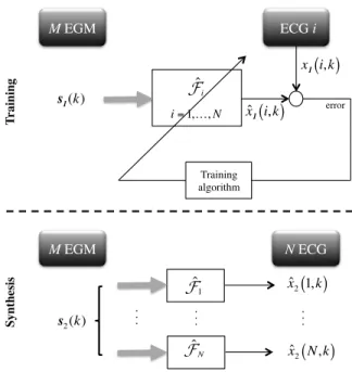
The estimation of F can be performed by a classical two-step procedure, including a training two-step and a synthesis two-step as depicted in Figure 1.
1) Training step: The objective of this step is to identify
the transfer function F, specific to each patient, by using a couple of learning datasets s1(k) (M EGM leads) and x1(k) (N ECG leads), of length L1. N different Multi-In Single-Out (MISO) systems (or transfer functions), F1,F2, ...,FN, between the M-rows input vector s1(k) and each row of the output vector x1(k), namely x1(i, k), are identified. Typically, the training step can be performed during the implantation, or whenever s1(k) and x1(k) can be simultaneously acquired.
2) Synthesis step: It is devoted to the follow-up of the
patient during a remote monitoring session, or during the regular in-hospital visits. In the latter case, a new EGM dataset s2(k), of length L2, is continuously measured and acquired by the device and used to synthesize a surface ECGxˆ2(i, k), by using the estimates ˆFi, for i= 1, . . ., N , such that:
ˆ x2(i, k) = ˆFi(s2(k)), k = 1, ..., L2. (2) M EGM! ECG i! T rai n in g! x 1
( )
i, k ˆ !i i= 1,…, N xˆ 1( )
i, k error! Training algorithm! M EGM! N ECG! S yn th es is ! s1(k) ˆ !N ˆ !1 . . . ! ˆ x 2(
1, k)
ˆ x 2(
N, k)
. . . ! s 2(k) . . . !Fig. 1. Methodology for the training and the synthesis steps in the case of the direct method.
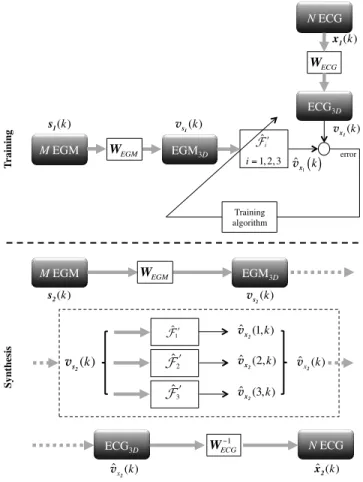
B. Indirect method
The principle of the indirect method is depicted in Fig-ure 2. The main difference relies on the computation of 3D representations of the surface (ECG3D) and intracardiac (EGM3D) electrical activities of the heart, from the available ECG and EGM signals, through linear transformations WECG and WEGM, respectively. Transfer function F′ will thus be estimated between EGM3D and ECG3D, which will be respectively denoted vs1(k) and vx1(k). This indirect method
implies the application of a specific pre-processing approach for the training and synthesis steps.
1) Three-Dimensional representation of the cardiac
elec-trical activity: Contrary to the standard 12-lead ECG, the
analysis based on beat loops has been found to i) better compensate the changes in the electrical axis caused by various extracardiac factors [10], such as respiration, body position, electrode positioning, and so forth, ii) give a compact repre-sentation of the cardiac electrical activity, minimizing storage needs, and iii) provide a solution to the time synchronization problem which arises in cardiac data.
In [5], we evaluated four different approaches to perform the calculation of the EGM3D and the ECG3D: Principal Component Analysis (PCA) [12], Robust Principal Component Analysis (RobPCA) [13], Independent Component Analysis based on Second Order statistics (ICASO) [14] and Indepen-dent Component Analysis based on Fourth Order statistics (ICAFO) [15]. We showed that the results can be considered equivalent and that a classical PCA is a satisfactory solution. PCA has thus been retained in this work.
2) Training step: vs1(k) and vx1(k) can be computed
directly from the first datasets of ECG and EGM, s1(k) and x1(k), by using the following equations:
vs1(k) = WEGM s1(k), k = 1, ..., L1 (3) vx1(k) = WECGx1(k), k = 1, ..., L1 (4)
T rai n in g! error! Training algorithm! vs 1(k) WEGM M EGM! s1(k) WECG N ECG! x1(k) v x1(k) ˆvx1( )k S yn th es is ! ˆ ! !i i= 1, 2, 3 M EGM! s2(k) WEGM EGM 3D! vs 2(k) ˆ !3! vˆx2(3, k) N ECG! ˆ x 2(k) WECG!1 ECG3D! ˆ vx 2(k) ˆ !2! vˆx 2(2, k) ˆ vx 2(1, k) ˆ ! !1 v s2(k) ˆ vx 2(k) EGM3D! ECG3D!
Fig. 2. Methodology for the training and the synthesis steps in the case of the indirect method.
where WEGM and WECGare(3×M ) and (3×N ) matrices, vs1(k) and vx1(k) are (3×L1), in the general case.
Then, the problem can now be modeled as follows: vx1(k) = F′(vs1(k)) + b(k), (5) where the output vx1(k) is considered as an unspecified non linear functionF′ of the inputs vs
1(k) plus an additive white
noise b(k).
Contrary to the direct case, only three different MISO systems, F′
1,F2′ and F3′, between the 3-rows input vector vs1(k) and each row of the output vector vx1(k), namely vx1(i, k), have to be estimated during the training step.
3) Synthesis step: It is composed of three phases:
• WEGM is applied to EGM s2(k), which provides the (3 × L2) EGM3D matrix vs2(k).
• The (3 × L2) ECG3D matrix ˆvx2(k) is computed by using ˆF′
1, ˆF2′ and ˆF3′, learnt during the training step. • The N -lead ECG ˆx2(k) is obtained by multiplying the
pseudo-inverse of the linear transform WECG with the estimated ECG3D vˆx2(k).
4) Particular case: In the general case where M ≥ 3,
PCA is applied to reduce and to orthogonalize the EGM data and we take into account the three largest eigenvalues of the covariance matrix. In the particular case where M = 2, the PCA is not used to reduce the number of components, but just to orthogonalize the EGM data and the two eigenvalues of the covariance matrix are taken into account, so that WEGM is
(2×M ) and vs1(k) and vs2(k) are (2 × L1) and (2 × L2)
respectively.
C. Non linear estimation method
In both cases (direct and indirect methods), the transfer function is modeled as a nonlinear function, based on a Time Delay artificial Neural Network (TDNN). It is well-known that feed-forward Artificial Neural Networks (ANN) with an input layer, a single hidden layer, and an output layer may be used as universal function approximators, under very general conditions for the activation functions [11], [16]. TDNN are a particular implementation of feed-forward ANN, in which delayed versions of the input signals are presented at the input layer of the network. TDNN have thus an extended capability for time series processing, with respect to feed-forward ANNs, since they include a representation of the d past samples of each input signal. In this work, each TDNN is defined with an input layer of NI = N × d samples, a hidden layer of NH neurons with a sigmoid activation function and one linear output neuron. The implementation is based on the approach proposed by D. MacKay [17], to improve the generalization of the procedure and to avoid overfitting.
D. Linear approach
The performance provided by the two TDNN-based ap-proaches will be compared with a classical linear approach. Indeed, the transfer function between an input y(k) and an output z(k) is commonly supposed to be a linear Wiener filter h, such that:
z(k) = (h ∗ y)(k) (6)
where ∗ is the convolution operation and h(k) = [h(0), . . ., h(Lh))] is the impulse response of a linear time invariant filter of length Lh. Least square estimation of h leads to the classical relation:
ˆ h= R−1
zzRzy (7)
where Rzz is the autocorrelation matrix of the output, Rzy is the intercorrelation matrix between the output and the input and ˆh is the estimate of h. Several implementations, block or recursive, can be applied to find the optimal estimator of h. In the recursive way, Least Mean Square (LMS), Normalized Least Mean Square (NLMS) or Recursive Least Square (RLS) algorithms have been proposed. Best results were obtained with the RLS approach, moreover known to exhibit fast convergence and the exact implementation of the block form. In the direct case, the filter represents the transfer function between EGM and ECG signals (as in [9]). During the training step, N MISO filters have to be computed, between the input EGM vector s1(k) (y(k) = s1(k)) and each row of the output ECG vector x1(k) (z(k) = x1(i, k) for i = 1, . . ., N ). In the indirect case, the filter represents the transfer function between EGM3Dand ECG3Dsignals [4]. During the training step, three MISO filters have to be computed, between the input EGM3D vector vs1(k) (y(k) = vs1(k)) and each row of the output ECG3D vector vx1(k) (z(k) = vx1(i, k) for i= 1, . . ., 3).
III. PRESENTATION OF THE DATABASE
A dataset issued from 15 patients (P1 to P15) is used to evaluate the performance of the above-mentioned ECG recon-struction methods. The ECG and EGM were simultaneously recorded with a GE Cardiolab station during the implant of an ICD with an initial sampling rate equal to1000 Hz and then subsampled at 128 Hz and low-pass filtered at 45 Hz. Each record of the database is composed of:
• 12 standard surface ECG channels, namely leads I, II, III, aVR, aVL, aVF, V1 to V6;
• Four EGM channels: BipA acquired using a bipolar measure between the tip and proximal electrodes of the atrial lead; BipV, a bipolar measurement between the tip and proximal electrodes of the ventricular pacing lead; ProxA between the proximal electrode of the atrial lead and the pacemaker can and ProxV between the proximal electrode of the ventricular lead and the pacemaker can. Three EGM configurations will be considered:
• ’Bip’: using the two bipolar channels BipA and BipV (M = 2);
• ’Prox’: using the two proximal ProxA and ProxV (M = 2);
• ’Bip+Prox’: using the four EGM (M = 4).
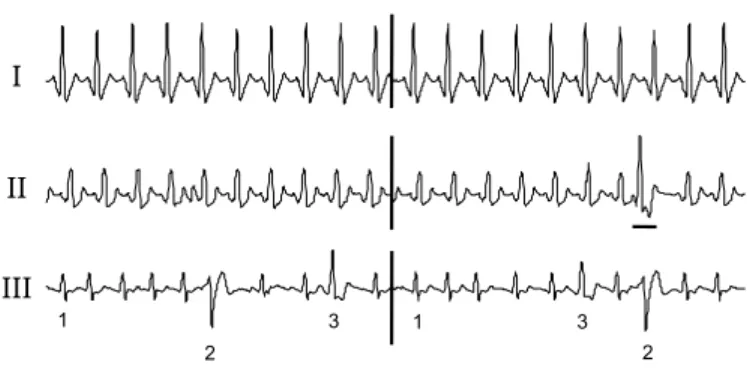
Each patient file has been segmented into two blocks: the first one, of length L1, containing ntheartbeats of concurrent ECG and EGM signals, is used during the training step, and a different second block, of length L2, with ns beats, is devoted to the synthesis step and performance evaluation. The 15 patient records have been classified into three categories, according to their beat morphologies (Fig. 3):
• Type I: the surface ECG contains only one beat morphol-ogy (P1 to P10);
• Type II: the surface ECG contains one prevailing beat morphology, with presence of ventricular ectopic beats (P11 to P13). Ectopic beats are only included in the testing set;
• Type III: at least three different beat morphologies com-pose the ECG (P14 and P15). Each of them are present both in the training and testing sets.
I II III 1 1 2 2 3 3
Fig. 3. Example of signals (one derivation of ECG) of Type I, Type II and Type III.
IV. RESULTS
The behavior of the non linear estimation methods depends on the values of the TDNN parameters, that are optimized on
the training dataset in the first part of this section. In a second part, we present the results obtained on the synthesis dataset as a function of the EGM leads and the type of patients. We evaluate the two TDNN-based methods (direct and indirect) and compare the results with an RLS filter (direct and indirect). This leads to four different methods, denoted by:
• D_TDNN: Direct method and estimation of the transfer function by TDNN
• I_TDNN: Indirect method and estimation of the transfer function by TDNN
• D_RLS: Direct method and estimation of the transfer function by a RLS filter
• I_RLS: Indirect method and estimation of the transfer function by a RLS filter.
The last part of this section presents the practical importance of the proposed methodology, in the real configuration of an implantable device. We study the effect of the reconstruction process on parameters extracted from the ECG and in a diagnosis purpose, since the ECG is also used in practice for the control of the device and for arrhythmia detection.
A. Optimization of the parameters of the network
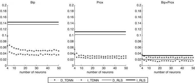
Performance of the two TDNN-based methods (direct and indirect) are highly dependent on the adjustment of the NN parameters: the delay d, the number of neurons NH and the length L1 of the training set. The delay d has been optimized in a previous work to 50 ms (d = 4 samples) [18]. For the two others parameters, a bootstrap analysis is performed on the database. Mean Square Errors (MSE) between the 12 leads of the real ECG and the synthesized ECG have been computed as the function of the number of neurons NH∈ {4, 6, ..., 50} and the number of beats in the training set nt∈ {2, 3, ..., 10}. Due to length duration of the training data set, ten beats were the maximal possible value.
Figure 4 shows that the MSE decreases when the number of neurons NH increases, with a ’plateau’ phase above 20 neurons. Regarding the influence of the number of beats nt, Figure 5 shows that MSE decreases when this number is increasing. From these previous experiments and for the following, the number of neurons NH and the number nt of beats in the training set are tuned to 20 and 10 respectively.
B. Performance analysis of the synthesized ECG
The quality of the synthesized ECG obtained from the four methods has been evaluated by calculating the correlation coefficient between the synthesized ECG and the real ECG, for all the available patients, and for all EGM configurations. Results have been grouped by the type of recording, as depicted in Fig. 3 and are presented on Fig. 6.
1) Analysis of the results as a function of the recording type:
The highest performance is obtained for Type I (sinus rhythm), whatever the reconstruction method and the EGM configura-tion. Then still high correlation coefficients are obtained with patients of Type III, containing polymorphic beat sequences, which means that all the heartbeats are well estimated.
Regarding recordings of Type II, correlation coefficient values are lower. This is mainly due to the ectopic beat, not
4 10 20 30 40 50 0 0.02 0.04 0.06 0.08 0.1 0.12 0.14 0.16 0.18 0.2 Bip number of neurons 4 10 20 30 40 50 0 0.02 0.04 0.06 0.08 0.1 0.12 0.14 0.16 0.18 0.2 Prox number of neurons 4 10 20 30 40 50 0 0.02 0.04 0.06 0.08 0.1 0.12 0.14 0.16 0.18 0.2 Bip+Prox number of neurons D_TDNN I_TDNN D_RLS I_RLS
Fig. 4. Evolution of mean square errors (in mV2) between the real ECG and the synthesized ECG: Influence of the number of neurons.
D_TDNN I_TDNN D_RLS I_RLS 2 3 4 5 6 7 8 9 10 0 0.02 0.04 0.06 0.08 0.1 0.12 0.14 0.16 0.18 0.2 Bip number of beats 2 3 4 5 6 7 8 9 10 0 0.02 0.04 0.06 0.08 0.1 0.12 0.14 0.16 0.18 0.2 Prox number of beats 2 3 4 5 6 7 8 9 10 0 0.02 0.04 0.06 0.08 0.1 0.12 0.14 0.16 0.18 0.2 Bip+Prox number of beats
Fig. 5. Evolution of mean square errors (in mV2) between the real ECG and the synthesized ECG: Influence of the number of beats in the training set.
Type I Type II Type III Total 0 0.2 0.4 0.6 0.8 1 Bip
Type I Type II Type III Total 0 0.2 0.4 0.6 0.8 1 Prox
Type I Type II Type III Total 0 0.2 0.4 0.6 0.8 1 Bip+Prox Total 0 D TDNN ITDNN data3 data4 D_TDNN I_TDNN D_RLS I_RLS Bip+Prox Prox Bip
Fig. 6. Correlation coefficients calculated after synthesis of 12 ECG for the three types of patients, with the three configurations of EGM, using the four different methods.
included in the training set, which is not correctly reproduced. It is important to notice that this is a particularly difficult case. This result shows that unfortunately none of the evaluated methods is able to estimate the true transfer function when using a limited number of beat morphologies in the training set. However, the TDNN approaches provide a slightly higher performance (see section IV.B.3).
2) Selection of the EGM configuration: The best
perfor-mances are obtained with the configuration ’Bip+Prox’ what-ever the method. We can also observe that configuration ’Bip’ provides the lowest performances. Finally, results obtained with ’Prox’ are very interesting since they show that this configuration, using only two electrodes, allows to obtain almost the same results that the configuration ’Bip+Prox’, using four electrodes.
3) Comparison of the synthesis methods: Considering the
whole database, the best correlation coefficients are obtained with the D_TDNN method, in the configuration ’Bip+Prox’, leading to 0.99 for Type I, 0.84 for Type II and 0.95 for Type III. Furthermore, TDNN-based approaches provide glob-ally the best correlation coefficients compared to the RLS-based approaches, but the gain in performance is limited for configurations ’Prox’ and ’Bip+Prox’. However, in the configuration ’Bip’, the difference between TDNN and RLS is more important (this case will be detailed in the next section). In addition, D_TDNN provides, in most of the cases, slightly higher performances than I_TDNN. However, I_TDNN can be considered as a good compromise since its complexity is lower (identification of 3 transfer functions for I_TDNN and 12 transfer functions for D_TDNN) and its performances are equivalent.
C. Quantitative and qualitative performances in the real con-figuration of an implantable device
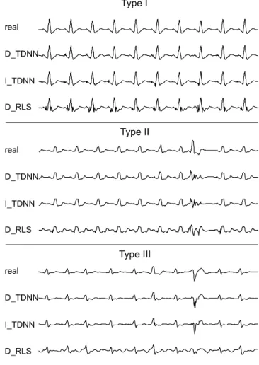
Up to now, we have considered the reconstruction for a research protocol. This section is now devoted to the real industrial case, where only 3 ECG leads are generally ob-served (and assumed sufficient during the follow-up process). Concerning the EGM, only 2 bipolar leads are often used in practice, which corresponds to a difficult configuration, as demonstrated in section IV-B2. By comparing three of the four methods (D_TDNN, I_TDNN and D_RLS) and by considering all the patients, a quantitative and a qualitative analysis have been performed on three ECG leads (I, II and V1), containing 10 heartbeats. Let us mention that in a previous work, we have shown that performances do not depend on the ECG lead which is synthesized [4].
1) A typical reconstruction example: As an illustration,
Figure 7 shows an example of lead I, synthesized with the three different methods. Results show the superiority of the TDNN-based approaches. RLS synthesizes a small high frequency reconstruction noise around each QRS of the patient of Type I and fails in reconstructing the three different morphologies of the patient of Type III. With the patient of Type II, sinus rhythm is still better estimated with the two TDNN approaches. However, results also show that the three methods fail to reconstruct the premature ventricular complexes (PVC),
not included into the training set. Nevertheless, the synthesized beat is clearly different than the sinus beats and could be interpreted, by an automatic system, as a PVB.
Type I Type II Type III real D_TDNN I_TDNN D_RLS real D_TDNN I_TDNN D_RLS real D_TDNN I_TDNN D_RLS
Fig. 7. Examples of synthesized ECG (lead DI) for a patient of each of the three types, using two bipolar EGM.
2) Quantitative evaluation: We propose now to evaluate the
quality of the synthesized ECG by comparing feature values extracted from the real ECG and from the synthesized ECG. The objective is to appreciate if the reconstruction process modifies some of the main parameters generally measured on the ECG signal for diagnosis purposes. It is well-known that the QRS duration and amplitude of the R wave are part of such important features and moreover can be used for the adjustment of the implantable device. In the same manner, heart rate variability and measurement of the ST segment are important for patient follow-up, the ST segment being a crucial parameter for ischemia monitoring.
The RR interval, QRS durations and R wave and ST seg-ment (measured 60 ms after J point and using as a reference the mean value of the PR interval) magnitudes have been extracted from real and synthesized ECGs using a software developed in our laboratory [19]. Figure 8 shows boxplots of the absolute error (median and interquartile ranges) measured for each beat between parameters obtained from the real ECG and the different synthesized ECG.
Results are globally in accordance with those reported in the previous section after computation of the correlation
0 0.01 0.02 0.03 0.04 1 2 3 Type I 0 0.01 0.02 0.03 0.04 1 2 3 Type II 0 0.01 0.02 0.03 0.04 1 2 3 Type III 0 0.02 0.04 0.06 1 2 3 Type I 0 0.02 0.04 0.06 1 2 3 Type II 0 0.02 0.04 0.06 1 2 3 Type III 0 0.05 0.1 0.15 0.2 1 2 3 Type I 0 0.05 0.1 0.15 0.2 1 2 3 Type II 0 0.05 0.1 0.15 0.2 1 2 3 Type III 0 0.05 0.1 0.15 0.2 1 2 3 Type I 0 0.05 0.1 0.15 0.2 1 2 3 Type II 0 0.05 0.1 0.15 0.2 1 2 3 Type III Abs. Err. of RR interval (s) Abs. Err. of R magnitude (mV)
Abs. Err. of QRS duration (s) Abs. Err. of ST magnitude (mV)
D_TD NN I_TDN N D_RL S D_TD NN I_TDN N D_RL S D_TD NN I_TDN N D_RL S D_TD NN I_TDN N D_RL S D_TD NN I_TDN N D_RL S D_TD NN I_TDN N D_RL S D_TD NN I_TDN N D_RL S D_TD NN I_TDN N D_RL S D_TD NN I_TDN N D_RL S D_TD NN I_TDN N D_RL S D_TD NN I_TDN N D_RL S D_TD NN I_TDN N D_RL S
Fig. 8. Boxplots of the absolute error (median and interquartile ranges) between values of RR interval, R magnitude, QRS duration and ST magnitude extracted from the real ECG and from the synthesized ECG, for three different approaches: D_TDNN, I_TDNN and D_RLS. Errors have been computed on all the beats of three leads (I, II and V1) and are grouped by type of patients.
coefficient. As already stressed in Figure 7, performances obtained with D_TDNN and I_TDNN are generally close and superior to performances of D_RLS, for which the measured dispersion is always higher. Likewise, best results are obtained for Type I. However, differences of performances that were observed between Types II and III are less important. This might be explained by the reduced training set in Type III, which makes the generalization of the transfer function sub-optimal. This point has a direct influence on the quality of the features extracted from the synthesized ECG. For instance, we observe that the RR interval is well reproduced, with median errors always lower than 5 ms (except for the RLS method on Type III), the D_TDNN method providing always the lowest dispersion. Regarding the errors in reproducing amplitude parameters (R wave and ST segment), median errors are still acceptable, with values around 50 µV . Finally, the estimation of the QRS duration produced median errors around 15 ms.
3) Qualitative evaluation: In order to obtain a clinical
appreciation of the results, beyond numerical results, we requested a cardiologist of the Rennes Hospital to perform a blinded qualitative evaluation of the synthesized ECG.
For each of the patients, 4 different ECG (the real ECG and three synthesized ECG using D_TDNN, I_TDNN and D_RLS), were shown to the cardiologist. He has been asked to mark, out of 10, each of the synthetic ECG, globally for the three leads, related to the real ECG, from two points of view:
• The first should reflect the visual quality of the synthe-sized ECG. The whole signal has been analyzed: QRS morphology, P wave and also baseline.
• The second should evaluate the capability to make the right diagnosis, the database containing several arrhyth-mias or conduction defects (PVC, bundle-branch blocks, atrial fibrillation, ...).
Type I Type II Type III
0 2 4 6 8 10 Visual quality
Type I Type II Type III
0 2 4 6 8 10 Diagnostic D_TDNN I_TDNN D_RLS
Fig. 9. Results of the qualitative evaluation (marks out of 10) for patients of Types I, II and III (visual quality: top, diagnosis: bottom).
Results are presented in Figure 9. Firstly, we observe a good agreement between scores obtained by the visual quality
analysis and by the capability to give the right diagnosis (same classification of the methods). In addition, results are in accordance with conclusions of the quantitative analysis since no significant differences between the direct method (D_TDNN) and the indirect method (I_TDNN) were observed for the proposed TDNN approach. Again, performances of the two TDNN-based methods are judged superior to the D_RLS, for the three types of patients. As already reported in this communication, worse results are obtained with patients of Type II. Finally, it is worth to mention that scores of diagnosis are always higher than those of visual quality. In other words, even if the signal is not always correctly reconstructed, the diagnosis may be preserved.
V. CONCLUSION
This paper proposes a methodology to synthesize a standard 12-lead ECG from a set of EGM leads, for implanted patients, which is of main practical importance in cardiology. For this purpose, two methods, a direct and an indirect, based on a dynamic TDNN, are proposed and evaluated in this study. Experiments show that four main issues are of concern when performing ECG reconstruction. Firstly, a quantitative comparison, conducted on a database issued from 15 patients, shows that performances of both TDNN-based methods are equivalent and outperform the RLS approach. However, the direct method requires the learning of 12 transfer functions, whereas the indirect method only requires three transfer func-tions. It is worth to notice that, in practice, it is also possible to compute only eight transfer functions and derive the other four by calculations, since only two of the six extremity leads are independent. Whatever the approach direct or indirect, the transfer functions are patient specific and must be trained either during the implantation or the day just after by collecting as set of synchronous ECG and EGM, eventually by using the telemetric system of the device.
Secondly, interesting results were observed for patients with sinus rhythm or with polymorphic beats if all the beat morphologies are present in the training set (Types I and III). When ectopic complexes are not included in the training set (Type II), both methods show limitations on the reproduction of PVC. However, the synthesized morphologies still remain very different from sinus beats, preserving at least the possi-bility of identifying a pathological beat.
Thirdly, results have also been presented as a function of the number and the type of EGM leads. As expected, the best reconstructions are obtained using two bipolar and two proximal leads, but we also demonstrated that the two proximal electrodes provide almost the same results.
Finally, we have shown that the industrial configuration, using only two bipolar EGM, leads to quantitative and quali-tative efficient performances. These interesting results suggest that the proposed TDNN-based reconstruction module could be embedded into an ICD.
It should be noted that the long term validity of this recon-struction relies on the hypothesis that the ECG morphology is stable over time. This hypothesis can be assumed to hold in healthy subjects and we recently verified this stability
in different recording conditions [20], [21]. However, this may not be the case in implanted patients, who may present ECG modifications as a consequence of cardiac remodeling, clinical evolution or transient phenomena (new medication, . . .). These factors represent the main limitations of any ECG reconstruction method from EGM data. One way to minimize the effects of these factors would be to re-estimate the transfer function during the required follow-up visits at the hospital.
This work also opens the way to new telecardiology chal-lenges, such as the optimal management of cardiac rhythm pathologies, the follow-up of implanted patients [22], [23], and the continuous control of implantable devices [24]. Indeed, recent studies have demonstrated the interest of a daily data transmission from the implantable device, through a wireless remote monitoring system, to improve the care of cardiac device recipients. It was also claimed in [25] that ambulatory monitoring of the electrocardiogram is an important comple-ment to pacemaker follow-up, particularly about changes in the ST segment of the ECG.
ACKNOWLEDGMENT
The authors acknowledge Professor François Carré from the Rennes Hospital for his participation to the clinical evaluation of this study.
REFERENCES
[1] V. L. Roger, A. S. Go, D. M. Lloyd-Jones, R. J. Adams, J. D. Berry, T. M. Brown, M. R. Carnethon, S. Dai, G. de Simone, E. S. Ford et al., “Heart disease and stroke statistics - 2011 Update. a report from the American Heart Association,” Circulation, vol. 123, no. 4, pp. e18–e209, 2011.
[2] M. Gentil, F. Porée, A. I. Hernández, and G. Carrault, “Surface elec-trocardiogram reconstruction from cardiac prothesis electrograms,” in
EMBEC05, Prague, Czech Republic, 2005, pp. 2028F1–6.
[3] A. Kachenoura, F. Porée, A. I. Hernández, and G. Carrault, “Surface ECG reconstruction from intracardiac EGM: a PCA-vectocardiogram method,” in Asilomar Conference on Signals, Systems, and Computers
2007, Pacific Grove, USA, 2007, pp. 761–4.
[4] ——, “Using intracardiac vectorcardiographic loop for surface ECG synthesis,” EURASIP Journal on Advances in Signal Processing, 2008:410630.
[5] A. Kachenoura, F. Porée, G. Carrault, and A. I. Hernández, “Comparison of four estimators of the 3D cardiac electrical activity for surface ecg synthesis from intracardiac recordings,” in ICASSP’09, Taïpei, Taïwan, 2009, pp. 485–8.
[6] ——, “Non-linear 12-lead ECG synthesis from two intracardiac record-ings,” in Computers in Cardiology, 2009, Park City, USA, 2009. [7] S. F. Saba, J. L. Williams, and G. S. Mendenhall,
“Electrocardio-gram reconstruction from implanted device electro“Electrocardio-grams,” Patent US 2009/0 187 097 A1, July, 2009.
[8] G. S. Mendenhall and S. Saba, “12-lead surface electrocardiogram reconstruction from implanted devices,” Europace, vol. 12, no. 7, pp. 991–8, 2010.
[9] G. Mendenhall, “Implantable and surface electrocardiography: comple-mentary technologies,” J. Electrocardiol., vol. 43, no. 4, pp. 619–23, 2010.
[10] F. Castells, P. Laguna, L. Sörnmo, A. Bollmann, and J. Roig, “Principal component analysis in ECG signal processing,” EURASIP Journal on
Advances in Signal Processing, 2007:74580.
[11] K. Hornik and M. Stinchcombe, “Multilayer feedforward networks are universal approximators,” Neural Networks, vol. 2, pp. 359–66, 1989. [12] K. I. Diamantaras and S. Y. Kung, Principal Component Neural
Net-works: Theory and Applications. New York, USA: Wiley-Interscience,
1996.
[13] A. Belouchrani and A. Cichocki, “Robust whitening procedure in blind source separation context,” Electronics Letters, vol. 36, pp. 2050–53, 2000.
[14] A. Belouchrani, K. Abed-Meraim, J.-F. Cardoso, and E. Moulines, “A blind source separation technique using second-order statistics,” IEEE
Trans. Signal Process., vol. 45, pp. 434–44, 1997.
[15] P. Comon, “Independent component analysis, a new concept?” Signal
Processing, Elsevier, vol. 36, pp. 287–314, 1994.
[16] C. Vásquez, A. I. Hernández, F. Mora, G. Carrault, and G. Passariello, “Atrial activity enhancement by wiener filtering using an artificial neural network,” IEEE Trans. Biomed. Eng., vol. 48, pp. 940–4, 2001. [17] D. J. C. MacKay, “Bayesian interpolation,” Neural Computation, vol. 4,
pp. 415–47, 1992.
[18] F. Porée, G. Carrault, A. Kachenoura, and A. I. Hernández, “Recon-struction of a surface electrocardiogram from an endocardial electrogram using non-linear filtering,” Patent US 2010/0 256 511 A1, October, 2010. [19] J. Dumont, A. I. Hernández, and G. Carrault, “Improving ECG beats delineation with an evolutionary optimization process,” IEEE Trans.
Biomed. Eng., vol. 57, pp. 607–15, 2010.
[20] F. Porée, J. Bansard, G. Kervio, and G. Carrault, “Stability analysis of the 12-lead ECG morphology in different physiological conditions of interest for biometric applications,” in Computers in Cardiology, 2009. IEEE, 2009, pp. 285–8.
[21] F. Porée, A. Gallix, and G. Carrault, “Biometric identification of indi-viduals based on ECG. Which conditions?” in Computing in Cardiology,
2011. IEEE, 2011, pp. 761–4.
[22] M. Guéguin, E. Roux, A. I. Hernández, F. Porée, P. Mabo, L. Grain-dorge, and G. Carrault, “Exploring time series retrieved from cardiac implantable devices for optimizing patient follow-up,” IEEE Trans.
Biomed. Eng., vol. 55, pp. 2343–52, 2008.
[23] V. Le Rolle, D. Ojeda, and A. Hernández, “Embedding a cardiac pulsatile model into an integrated model of the cardiovascular regulation for heart failure followup,” IEEE Trans. Biomed. Eng., vol. 58, no. 10, pp. 2982–2986, 2011.
[24] P. Mabo, F. Victor, P. Bazin, S. Ahres, D. Babuty, A. Da Costa, D. Binet, and J. C. Daubert, “A randomized trial of long-term remote monitoring of pacemaker recipients (the compas trial),” European heart journal, vol. 33, no. 9, pp. 1105–11, 2007.
[25] D. L. Janosik, R. M. Redd, T. A. Buckingham, R. I. Blum, R. D. Wiens, and H. L. Kennedy, “Utility of ambulatory electrocardiography in detecting pacemaker dysfunction in the early postimplantation period,”
The American Journal of Cardiology, vol. 60, no. 13, pp. 1030–1035,