HAL Id: hal-02101848
https://hal-lara.archives-ouvertes.fr/hal-02101848
Submitted on 17 Apr 2019HAL is a multi-disciplinary open access archive for the deposit and dissemination of sci-entific research documents, whether they are pub-lished or not. The documents may come from teaching and research institutions in France or
L’archive ouverte pluridisciplinaire HAL, est destinée au dépôt et à la diffusion de documents scientifiques de niveau recherche, publiés ou non, émanant des établissements d’enseignement et de recherche français ou étrangers, des laboratoires
Nested Circular Intervals: A Model for Barrier
Placement in Single-Program, Multiple-Data Codes with
Nested Loops.
Alain Darte, Robert Schreiber
To cite this version:
Alain Darte, Robert Schreiber. Nested Circular Intervals: A Model for Barrier Placement in Single-Program, Multiple-Data Codes with Nested Loops.. [Research Report] LIP RR-2004-57, Laboratoire de l’informatique du parallélisme. 2004, 2+27p. �hal-02101848�
Laboratoire de l’Informatique du Parallélisme
École Normale Supérieure de Lyon
Unité Mixte de Recherche CNRS-INRIA-ENS LYON-UCBL no5668
Nested Circular Intervals: A Model for
Barrier Placement in Single-Program,
Multiple-Data Codes with Nested Loops
Alain Darte and Robert Schreiber December 2004
Research Report No2004-57
École Normale Supérieure de Lyon
46 Allée d’Italie, 69364 Lyon Cedex 07, France Téléphone : +33(0)4.72.72.80.37 Télécopieur : +33(0)4.72.72.80.80 Adresse électronique : [email protected]
Nested Circular Intervals: A Model for Barrier Placement in
Single-Program, Multiple-Data Codes with Nested Loops
Alain Darte and Robert Schreiber December 2004
Abstract
We want to perform compile-time analysis of an SPMD program and place barriers in it to synchronize it correctly, minimizing the runtime cost of the synchronization. This is the barrier minimization problem. No full solution to the problem has been given previously.
Here we model the problem with a new combinatorial structure, a nested family of sets of circular intervals. We show that barrier minimization is equivalent to finding a hierarchy of minimum cardinality point sets that cut all intervals. For a single loop, modeled as a simple family of circular intervals, a linear-time algorithm is known. We extend this result, finding a linear-time solution for nested circular intervals families. This result solves the barrier minimization problem for general nested loops.
Keywords: Barrier synchronization, circular arc graph, nested circular interval graph, SPMD code, nested loops
R´esum´e
Le but de ce rapport est de montrer comment, apr`es une analyse statique de code, on peut synchroniser, `a l’aide de barri`eres, un programme de type SPMD tout en minimisant le temps de synchronisation `a l’ex´ecu-tion. C’est le probl`eme de minimisation des barri`eres. Aucune solution compl`ete n’a ´et´e donn´ee `a ce jour.
Nous mod´elisons le probl`eme par une nouvelle structure qui g´en´eralise la notion de graphe d’arcs circulaires, une famille d’intervalles circu-laires imbriqu´es. Nous montrons que le probl`eme de minimisation de barri`eres revient `a trouver une hi´erarchie d’ensembles, de tailles mini-males, de points du code (o`u placer les barri`eres) qui coupent Ż tous les intervalles. Pour une boucle simple, mod´elis´ee par un graphe d’arcs circulaires traditionnel, un algorithme lin´eaire est connu. Nous l’´eten-dons en un algorithme lin´eaire pour une famille d’intervalles circulaires imbriqu´es. Ce r´esultat r´esout le probl`eme de minimisation des barri`eres pour des boucles imbriqu´ees.
Mots-cl´es: Barri`ere de synchronisation, graphe d’arcs circulaires, graphe d’intervalles circulaires imbriqu´es, code SPMD, boucles imbriqu´ees
Contents
1 The problem of static optimization of barrier synchronization 2
2 The program model and a statement of the problem 4
2.1 Barriers, temporal partial ordering, dependence relations, and correctly synchronized programs . . . 5
2.2 Barriers, dependence level, and NCIF . . . 6
2.3 When is one solution better than another?. . . 9
3 Inner-loop barrier minimization 11
3.1 Straight-line code and minimum clique cover of an interval graph . . . 11
3.2 Inner-loop barrier minimization and the Hsu-Tsai algorithm . . . 12
4 Optimal barrier placement in nested loops of arbitrary structure 15
4.1 Basic bottom-up strategy . . . 15
4.2 Summarizing inner loop barrier placements: weaving/unraveling . . . 16
4.3 A linear-time algorithm to compute the function RIGHTMOST. . . 21
Nested Circular Intervals: A Model for Barrier Placement in
Single-Program, Multiple-Data Codes with Nested Loops
Alain Darte
CNRS, LIP, ENS Lyon 46, All´ee d’Italie, 69364 Lyon Cedex 07, France
Robert Schreiber
Hewlet Packard Laboratories, 1501 Page Mill Road,
Palo Alto USA [email protected]
16th December 2004
Abstract
We want to perform compile-time analysis of an SPMD program and place barriers in it to synchronize it correctly, minimizing the runtime cost of the synchronization. This is the barrier minimization problem. No full solution to the problem has been given previously.
Here we model the problem with a new combinatorial structure, a nested family of sets of circular intervals. We show that barrier minimization is equivalent to finding a hierarchy of min-imum cardinality point sets that cut all intervals. For a single loop, modeled as a simple family of circular intervals, a time algorithm is known. We extend this result, finding a linear-time solution for nested circular intervals families. This result solves the barrier minimization problem for general nested loops.
1
The problem of static optimization of barrier synchronization
A multithreaded program can exhibit interthread dependences. Synchronization statements must be used to ensure correct temporal ordering of accesses to shared data from different threads. Ex-plicit synchronization is a feature of thread programming (Java, POSIX), parallel shared memory models (OpenMP), and global address space languages (UPC [15], Co-Array Fortran [7]). Program-mers write explicit synchronization statements. Compilers, translators, and preprocessors generate them. In highly parallel machines, synchronization operations are time consuming [1]. It is there-fore important that we understand the problem of minimizing the cost of such synchronization. This paper takes a definite step in that direction, beyond what is present in the literature. In particular, we give for the first time a fast compiler algorithm for the optimal barrier placement problem for a program with arbitrary loop structure.
The barrier is the most common synchronization primitive. When any thread reaches a barrier, it waits there until all threads arrive, then all proceed. The barrier orders memory accesses: memory operations that precede the barrier must complete and be visible to all threads before those that follow. Even with the best of implementations, barrier synchronization is costly [11]. All threads wait for the slowest. Even if all arrive together, latency grows as log n with n threads. Finally, the semantics of a barrier generally must include a memory fence, which causes all memory operations that precede the barrier to be fully completed and globally visible before the start of any memory operation that follows the barrier.
Programmers and compilers add barriers to guarantee correctness. Experimental evidence [13] shows that programmers oversynchronize their codes. This is perhaps because it is hard to write correct parallel code, free of data races. We would therefore like to be able to minimize the cost of barriers through compiler optimization. A practical, automatic compiler barrier minimization algorithm would make it appreciably easier to write fast and correct parallel programs by hand and to implement other compiler code transformations, by allowing the programmer or other compiler phases to concentrate on correctness and rely on a later barrier minimization phase for reducing synchronization cost.
We call an algorithm correct if it places barriers so as to enforce all interthread dependences, and optimal if it is correct and among all correct barrier placements it places the fewest possible in the innermost loops, among such it places the fewest at the next higher level, etc. In their book on the implementation of data parallel languages, Quinn and Hatcher mention the barrier minimization problem [9]. They discuss algorithms for inner loops but not more complicated program regions. O’Boyle and St¨ohr [13] make several interesting contributions. Extending the work of Quinn and Hatcher, they give an optimal algorithm for an inner loop with worst-case complexity O(n2), where n is the number of dependences, and an algorithm that finds an optimal solution for any semiperfect loop nest, i.e., a set of nested loops with no more than one loop nested inside any other. Its complexity is quadratic in the number of statements and exponential in the depth of the nest. Finally, they give a recursive, greedy algorithm for an arbitrarily nested loop, and finally for a whole program. This algorithm is correct, and it will place the fewest possible barriers into innermost loops. But it doesn’t always minimize the number of barriers in any loop other than the innermost loops.
We describe (for the first time) and prove correct and optimal an algorithm for barrier min-imization in a loop nest of arbitrary structure. The algorithm is fast enough to be used in any practical compiler: it runs in time linear in the size of the program and the number of dependence relations it exhibits.
Remarks Note that, in this report, we don’t consider two important optimizations related to synchronization, a) statement reordering and b) the use of lighter weight synchronizations.
a) We have chosen to look at a model of the problem in which barriers must be placed without other changes to the program. In particular, we disallow reordering of statements and changes to the loop nesting structure, such as loop fusion and distribution might provide. We do not advocate this as a global program optimization strategy. Indeed, others have shown that such transformations may be beneficial. In the end, however, after such transformations have been applied by the optimizer, the problem that we address here remains: minimize the barriers without other code modifications. Barrier minimization with statement reordering is a scheduling problem. Barriers divide time into interbarrier epochs, and the problem is to schedule work into epochs such that the total length of the schedule is minimized. Callahan [5] and Allen, Callahan, and Kennedy [3] made basic contributions to the theory of program transformation to reduce schedule length. Note that statement reordering, even when legal, may not be advisable, principally because it can worsen memory performance, which is often a critical performance limiter. Thus, the problem at hand, nested loops with no reordering, is of considerable interest.
b) Some dependence relations do not require barriers: they are enforceable by lighter weight synchronization, such as event variable synchronization or point-to-point communication (see for example [14]). These dependences can be so enforced, and the code modified accordingly, before we consider the barrier minimization problem. It may be necessary, after this is done, to annotate the code so as to avoid the detection and enforcement (with a barrier) of a dependence that has
been synchronized by event variables. We ignore this possibility for the remainder of the paper, and assume that barrier is the only primitive used for synchronization.
2
The program model and a statement of the problem
We assume a program with multiple threads that share variables. Each thread executes a sepa-rate copy of an identical program (single-program, multiple data, or SPMD). Threads know their own thread identifier (mythread) and the number of threads (threads). By branching on mythread, arbitrarily complicated MIMD behavior is possible. The threads call a barrier routine to synchro-nize. Barriers divide time into epochs. The effects of memory writes in one epoch are visible to all references, by all threads, in the following epochs.
Clearly, if any thread hits a barrier then all threads must execute a barrier or there will be a deadlock, with some threads waiting forever. So in a correct program, all threads make the same number of barrier calls. We make a stronger assumption: following Aiken and Gay, we assume that the program is structurally correct [2], which means that all threads synchronize by calling the same barrier statement, at the same iteration of any containing loops. The simple way to understand this is as a prohibition on making a barrier control-dependent on any mythread-dependent condition. Structural correctness may be a language requirement as in the Titanium language [17]. Titanium uses the keyword single to allow a programmer to assert that a private variable takes only thread-independent values. We can also optimize programs in looser SPMD languages such as UPC [6] and Co-Array Fortran [12] if we discover at compile time that they have no structural correctness violations.
We don’t view structural correctness as a significant restriction on the programmer’s ability to express important and interesting parallel algorithms. Here’s why. Aiken and Gay presented empirical evidence that actual shared-memory parallel applications rarely violate structural cor-rectness, even in dialects that allow it. They implemented static single-valuedness analysis as well as the single keyword in an extension of the SPMD language Split-C [4]. In this dialect, they were able to implement and statically verify the structural correctness of a variety of typical parallel scientific benchmark codes (cholesky, fft, water, barnes, etc.) by making a small number of uses of single [2]. Also, structural correctness is a natural property of any SPMD implementation of a program written originally in a traditional fork/join model of parallelism such as OpenMP. Threads will synchronize with (one and the same) barrier at the end of each parallel construct.
We can analyze and optimize any program region consisting of a sequence of loops and state-ments, which we call a properly nested region. We can change any properly nested region into a single loop nest, by adding an artificial outer loop (with trip count one) around the region. We can, therefore, take the view from now on that the problem is to minimize barriers in some given loop nest. In a loop nest, the depth of any statement is the number of loops that contain it. The loop statement is itself a statement and has a depth: zero if it is the outermost loop. The nesting structure is a tree, with a node for each loop. The outermost loop is at the root, every other loop is a child of the loop that contains it. The height of a loop is zero if it is a leaf in the nesting tree, otherwise it is one greater than the height of its highest child.
We make the following assumptions:
• Loops have been normalized so that the loop counters are incremented by one. We don’t really need this, but it allows us to simply write i + 1 when we mean the next value of the loop index i.
in each branch first (as O’Boyle and St¨ohr do), before treating the rest of the loop nest. This is correct but sub-optimal. Therefore, our algorithm is optimal only for a loop nest with no dependences between statements in IF-THEN-ELSE.
• There are no zero-trip loops. This ensures that a barrier placed in the body of a loop L will enforce any dependence from a statement executed before L to another executed after L. Again, this assumption simplifies the discussion, but it is not really necessary for correctness. This because we can assume this property, solve the barrier placement problem, then re-analyze the program and determine those loops containing a barrier that enforces such a “long” dependence (from before the loop to after it) and that may possibly be zero-trip, and insert an alternative for the case where the loop does not execute, containing another barrier:
for (i = LB; i < UB; i++) { ... barrier; ...} if (UB <= LB) {barrier;}
2.1 Barriers, temporal partial ordering, dependence relations, and correctly
synchronized programs
Our problem is to place barriers to enforce interthread dependence relations. To reason about these, we need some preliminary notions. We denote by S(~iS) the operation that corresponds to the (static) statement S and the particular values of the loop counters, specified by the integer vector ~iS, for the loops, if any, in which S is nested. In an SPMD program, each operation S(~iS) has many instances, one for each thread that executes the portion of code that contains it. To distinguish between instances, we denote by S(tS,~iS) the instance of S(~iS) executed by the thread whose number or identifier is tS.
If statement instances s and t are executed by the same thread then we write s ≺seq t to
indicate that s precedes t in sequential control flow. On the other hand, the barrier B synchronizes
S(tS,~iS) and T (tT,~iT), instances from different threads, if there is an operation B(~iB) such that
S(tS,~iS) ≺seq B(tS,~iB) and B(tT,~iB) ≺seq T (tT,~iT). The two individual barrier calls B(tS,~iB) and
B(tT,~iB) are calls to the same operation B(~iB) of a single barrier B; because we target structurally correct programs, such calls always synchronize with one another.
For operations, let us write S(~iS) ≺seqT (~iT) if sequential control flow orders their instances on each individual thread. We say that the barrier B synchronizes operations S(~iS) and T (~iT) if there is an operation B(~iB) such that S(~iS) ≺seq B(~iB) ≺seq T (~iT). Formally, S(~iS) ≺seq T (~iT) is defined as follows. Let c be the number of loops that surround both of S and T . Then S(~iS) ≺seq T (~iT) if either ~iS is lexicographically smaller than ~iT in their first c components (those that refer to their common containing loops) or the two index vectors are equal in their first c components and S precedes T in the program text.
An interthread dependence relation RST between statements S and T is a set of pairs of oper-ations. At least one of S or T is a write to a shared variable. For each pair (S(~iS), T (~iT)) ∈ RST, there is some barrier in the source code that synchronizes them. And finally, there are instances of S(~iS) and T (~iT), not both on the same thread, that reference the same shared variable, or at least we cannot determine at compile time that they do not, so they must be correctly ordered in time. From now on, when we talk of dependences we shall mean these interthread dependences. A barrier B enforces a dependence R if it synchronizes every pair of operations in the relation. In this case, we have S(~iS) ≺seq B(~iB) ≺seqT (~iT), in other words, the barriers in the given SPMD pro-gram define a temporal partial order (sub-order of the order ≺seq) on operations, which determines
2.2 Barriers, dependence level, and NCIF
For our purposes, it is enough to analyze dependence, find the instance relations, ignore the in-trathread pairs, project each instance relation (that has interthread pairs) into a relation on oper-ations, and determine the loop, if any, that carries it. We informally introduce these ideas here, and define things carefully later. For now, consider the SPMD program fragment:
for (i = 0; i < n; i++) { for (j = 0; j < m; j++) {
b[i][j + m*mythread] = f(c[i][j + m*mythread]);
if (i > 0) a[i][j + m*mythread] = b[i-1][g(j + m*mythread)]; }
barrier; }
Consider the write of b[i][j+m*mythread] and the read of b[i-1][g(j+m*mythread)]. If the compiler cannot analyze the behavior of the indexing function g, it must assume that the thread that writes an element of b is different from the thread that reads this element – so this is an interthread (flow) dependence. The compiler can know, however, that the dependence relation consists of instances (s, t) for which the iteration vector if s is (i, j) and that of t is (i + 1, j0). Because the i loop is the outermost loop for which the dependent pairs occur in different loop iterations, we say that this loop carries the dependence and that the dependence is loop-carried.
The barrier in the example code enforces this dependence. There are other places where a barrier could be placed to do this. It could occur before the inner loop:
for (i = 0; i < n; i++) { barrier;
for (j = 0; j < m; j++) {
b[i][j + m*mythread] = f(c[i][j + m*mythread]);
if (i > 0) a[i][j + m*mythread] = b[i-1][g(j + m*mythread)]; }
}
It would also suffice to have a barrier in the inner loop: for (i = 0; i < n; i++) {
for (j = 0; j < m; j++) {
b[i][j + m*mythread] = f(c[i][j + m*mythread]);
if (i > 0) a[i][j + m*mythread] = b[i-1][g(j + m*mythread)]; barrier;
} }
This solution might be overkill, however. Clearly there are more barriers executed (assuming m > 1) than for the other solutions. On the other hand, if there were some other dependence, carried by the j loop or not carried by any loop, that required a barrier inside the j loop, then this might be the best way to also enforce to dependence involving the array b. This is the case, for example, in the code hereafter. Note that the inner-loop barrier enforces a flow loop independent (i.e., not carried by any loop) dependence involving the arraya, an antidependence on the arrayc, and also the flow dependence on the arrayb, by virtue of our certainty that the inner loop executes at least once for every iteration of the outer loop.
for (i = 0; i < n; i++) { for (j = 0; j < m; j++) {
b[i][j + m*mythread] = f(c[i][j + m*mythread]);
if (i > 0) a[i][j + m*mythread] = b[i-1][g(j + m*mythread)]; barrier;
if (mythread > 0) c[i][j + m*mythread] = 2 * a[i][j + m*(mythread-1)] }
}
We now define more formally the relations between barrier placements and loop-carried/loop-independent dependences. We consider a properly nested region, which is turned into a single loop nest, as above. A set of dependences between statement instances is found by analysis of the given loop nest. 1 The dependence relations between statement instances are projected into a set of relations between operations, each of which is either loop-independent or is carried at some loop level, as described next.
Consider a dependence from operation S(~i) to T (~j): we know that S(~i) ≺seq T (~j). Let c be
the number of loops that surround both S and T ; ~i and ~j have at least c components. We use the standard notion of dependence level [16]: if the first c components of ~i and ~j are equal, the dependence is loop-independent at level c, otherwise it is loop-carried at level k where k ≤ c is the largest integer such that the first k −1 components of ~i and ~j are equal. We view the statements of the program as laid out from the earliest (in program text order) on the left to the last on the right. Thus, “to the left of” and “leftmost” mean earlier and earliest (with respect to program text order). We describe the dependences as circular intervals, which we define below.
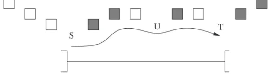
First consider the case of a loop-independent dependence. An example is depicted in Figure 1
from S to T , at level c = 1: a white box represents a DO, a grey box an ENDDO, the arrow from S to T represents the control flow. The dependence is represented by an open interval ]S, T [ (see the
U
S T
Figure 1: Interval for a loop-independent dependence (basic case).
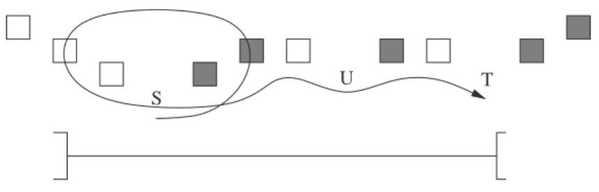
bottom of Figure1), and any barrier placed inside this interval enforces the dependence. All cases of loop-independent dependences can be represented by such an interval. For example, if we know that a loop containing S at depth ≥ c (i.e., not around T ) executes at least once before the control flow goes to T , we represent the dependence with a larger interval from the DO of this loop to T (see Figure2). If, likewise, a loop surrounding T iterates at least once before reaching T , then the interval is extended on the right to the appropriate ENDDO.
Now consider a loop-carried dependence. An example from S to T , of level k = 2, is depicted in Figure3where T strictly precedes S in the program text and jk= ik+ 1. The control points where a barrier needs to be inserted (and any such control point is fine) can be represented by a circular 1The mechanism and the precision of dependence analysis is not the subject of this paper, so we will not go into
any detail as to how the dependence relations are determined. We specify here how the dependences are represented, and analyze where barriers can be placed to enforce dependences.
U
S T
Figure 2: Case of an interval, for a loop-independent dependence, left-extended to a DO.
interval from S to T through the ENDDO and DO of the loop at depth k − 1 shared by S and T . In the example, this means that any barrier insertion between S and the ENDDO of the second loop, or between the DO of the second loop and T enforces this dependence. If, on the other hand,
k is 1, the interval would be extended through the ENDDO and DO of the first loop. Again, if we
know more about additional iterations of a loop deeper than k surrounding either S or T , we may be able to use a wider circular interval, whose endpoints may be a DO earlier than S (the fourth DO in the example) or an ENDDO after T (the ENDDO of the third loop in the example).
S T
Figure 3: Circular interval for loop-carried dependence (basic case).
A wrap-around dependence, which spans more than one full iteration of loop k, where k is the level of the dependence, can also be represented by an open interval from the DO at depth k − 1 to its ENDDO. Such a dependence can also simply be ignored if we know that the loop contains at least another dependence that will require a barrier anyway.
To summarize, we distinguish two types of dependence. A dependence can be:
Type A a loop-independent dependence at level k represented by an interval ]x, y[ where x (resp. y) is a statement or a DO (resp. ENDDO), x is textually before y, and x and y are surrounded by exactly k common loops: a barrier needs to be inserted textually after x and before y, and any such barrier does the job.
Type B a loop-carried dependence represented by an interval ]x, y[ and an integer k, where x (resp. y) is a statement or a DO (resp. ENDDO), x is textually after y, and they have at least k common loops: a barrier needs to be inserted textually after x and before the common surrounding ENDDO whose depth is k − 1, or after the common surrounding DO whose depth is k − 1 and before y, and any such placement is fine. (A wrap-around dependence is represented as a particular Type B dependence, from a DO to the corresponding ENDDO.) Thus, our model of the barrier placement problem is a linear arrangement of control points and a set of circular intervals. We refer to such a model as a nested circular interval family (NCIF). A barrier placement is equivalent to a set of points (at which to insert barrier statements) between
the control points of the NCIF. It is correct if each interval in the NCIF is “cut” by (i.e., contains) one or more barriers.
2.3 When is one solution better than another?
We represent the cost of a barrier placement P for a loop nest by a vertex-weighted tree T = cost(P ), whose structure is that of the nesting structure of the loop nest. Each vertex v (interior or leaf) has a weight b(v) given by the number of barriers in the strict body of the loop (i.e., not in a deeper loop) to which v corresponds. Define a partial order ¹ among tree costs as follows:
Definition 1 Let T and U be the tree costs of two barrier placements for a loop nest. Let t and u
be the roots of T and U , and (Ti)1≤i≤n and (Ui)1≤i≤n be the subtrees (rooted at the children of t
and u) of T and U . We say that T is less than or equal to U (denoted T ¹ U ) if
• Ti ¹ Ui, for each i, 1 ≤ i ≤ n,
• if, for each i, 1 ≤ i ≤ n, Ti= Ui, then b(t) ≤ b(u),
If T ¹ U and T 6= U , we say that T is less than U (denoted T ≺ U ).
Now we can compare barrier placements: P is better than Q if cost(P ) ≺ cost(Q). We say that a barrier placement P is optimal if it is correct and is as good or better than every other correct barrier placement. This definition of optimality is not the same thing as saying “there is no placement better than this one.” It asserts that an optimum cannot be incomparable with any other placement, but must be as good as or better than all others. Observe that the existence of optimal placements is not immediate, since the relation ¹ is only a partial order. The next lemma shows that optimal placements always exist. Moreover, the recursive definition of ¹ implies that, for a given loop L, all optimal placements have the same tree cost and that the restriction of any optimal placement for L to any loop L0 contained in L is optimal for L0. We can therefore talk about the cost of a loop nest, defined to be the tree-cost of any optimal placement.
Lemma 1 For any two solutions P and Q, there is a solution as good or better than both P and Q. Consequently, optimal solutions exist.
Proof. The proof is by induction on the height of the loop, i.e., the number of nested loops it contains.
For a loop L of height 0, i.e., for an innermost loop, P is as good or better than Q if P places no more barriers in L than Q. Thus, any two solution costs are comparable, and either P is better than Q (so use P ), or the converse (use Q), or they are equally good (use either).
For a loop L of height h > 0, containing the loops (Li)1≤i≤n, consider two solutions P and Q
such that P is not as good or better than Q and Q is not as good or better than P (otherwise, there is nothing to prove), i.e., two solutions whose tree costs are not comparable by ¹. Let T and U be their respective tree costs, and Pi and Qi be the restrictions of P and Q to Li, with tree costs Ti and Ui. By definition of ¹, there exist j and k, perhaps equal, such that Tj 6¹ Uj and Uk 6¹ Tk. By the induction hypothesis, there exist solutions Ri for every subtree Li, as good or better than both Pi and Qi. In particular, each Ri is a correct placement for Li, therefore they enforce all dependences not carried by L and not lying in the body of L. We can extend the local solutions
Ri to a solution R for L by placing a barrier after each statement in the body of L (this is brute force, but enough for what we want to prove). We have cost(Ri) ¹ Ti for all i, and cost(Rj) ≺ Tj (indeed, cost(Rj) = Tj is not possible since this would imply Tj ¹ Uj). Thus R is better than P . Similarly R is better than Q.
What we just proved is correct even if we restrict to the finite set of solutions that place in each loop at most as many barriers as statements plus one (i.e., one barrier between any two statements). Therefore, the fact that any two solutions have a common as good or better solution implies that
there are optimal solutions. ¥
Note that two placements with the same tree cost (even if they differ in the exact position of barriers inside the loops) lead to the same dynamic barrier count. The key point is that to get an optimal placement for a nest, one must select the right set of optimal placements for the contained loops. Consider the example in Figure 4 with dependences from G to A (carried by the outer
A B C D E F G H
Figure 4: A 2D example and its (unique here) optimal placement.
loop, i.e., with k = 1) and from C to F (loop-independent at level 1). The dependences internal to the inner loops are (A, D) and (C, B), as well as (E, H) and (G, F ). These allow for two local optima for each of the inner loops: a barrier may be placed just before B or just before D, and just before F or just before H. Clearly, there are four possible combinations of two local optima, but only the choice of barriers just before D and just before H leads to a global optimal, because with this choice (uniquely) of local optima, no barriers are needed at depth 1.
For completeness, let us point out that if every loop iterates at least twice whenever encoun-tered, an optimal placement executes the smallest possible number of barriers among all correct placements.
Lemma 2 If each loop internal to the nest iterates at least twice for each iteration of the surround-ing loop, then an optimal solution minimizes, among all correct placements, the number of barrier calls that occur at runtime.
Proof. It suffices to show that if Q, with tree cost U , is not optimal (in terms of ¹), then there exists a better solution P , with tree cost T ≺ U , such that P does not induce more dynamic barriers than Q.
Consider Q a solution for L with tree cost U , not optimal with respect to ¹. Let L0 be a loop of minimal height such that the restriction of Q to L0, with tree cost U0, is not optimal. By construction, U0is a subtree of U and all subtrees of U0are optimal tree costs for their corresponding subloops. Furthermore, for the solution Q, the number of barriers in the strict body of L0 (i.e.,
b(u) where u is the root of U0) is strictly larger than in any optimal solution for L0. Replace in Q
the barriers in L0 (i.e., in L0 and deeper) by the barriers of any optimal solution for L0. This gives a partially correct solution: all dependences are enforced except maybe some dependences that enter L0 or leave L0. To enforce them, add a barrier just before L0 and a barrier just after L0, so as to get a new correct solution P . The tree cost T of P is obtained by replacing in U the subtree U0 by the optimal subtree T0 of L0. The root t of T0 is such that b(t) ≤ b(u) − 1.
By construction, P is better than Q in terms of ¹ since b(t) < b(u). It remains to count the number of dynamic barriers induced by P and Q. There is no difference between P and Q, in terms of tree cost, for loops inside L0. So they have the same dynamic cost. This is the same for
all other loops, except for the strict body of L0 and for the loop strictly above L0. Consider any iteration of this loop: the difference between the number of dynamic barriers for Q and the number of dynamic barriers for P is N (b(u) − b(t)) − 2 where N is the number of iterations of L0 for this particular iteration of the surrounding loop. Since N ≥ 2 and b(t) − b(u) ≥ 1, P does not induce
more dynamic barriers than Q. ¥
3
Inner-loop barrier minimization
In this section, we recall results for one-dimensional cases: the case of a straight-line code and the case of a single innermost loop.
For a straight-line code (i.e., no loop), a simple greedy linear-time algorithm does the job: Find the first (leftmost) right endpoint of any interval, and cut with a barrier just to the left of this endpoint. Repeat while any uncut intervals remain. This technique was used by Quinn and Hatcher [9] and by O’Boyle and St¨ohr [13]. Next, these authors leverage this process to get a quadratic-time algorithm for simple loops: Try each position in the loop body for a first barrier, which cuts the circle making it a line; next apply the linear-time algorithm above to get the remaining barriers; and finally choose the solution with the fewest barriers.
Surprisingly, it seems that none of the previous work on barrier placement recognized that the problem for a straight-line code is nothing but the problem of finding a minimum clique cover in an interval graph. (The algorithm of [9, 13] is exactly the well-known greedy algorithm for this problem [8]). Generalized to an inner loop, the problem is to find a minimum linear clique in a circular interval family, for which there exists a very simple linear-time (thus better than quadratic) algorithm [10]. Our technique to solve optimally the case of general loops and to reduce the complexity of the barrier placement algorithm (even in cases for which an optimal algorithm has already been given) is based on this linear-time algorithm for finding a minimum linear clique cover in a circular interval family. We introduce these concepts and explain the corresponding algorithms next.
3.1 Straight-line code and minimum clique cover of an interval graph
In a straight-line code, only loop-independent dependences exist (dependences of type A). They correspond to intervals Ii = ]hi, ti[ where hi and ti are integers such that hi < ti, i.e., intervals on a line. The classical graph associated to intervals on a line is the so-called interval graph, an undirected graph with a vertex per interval and an edge between two intervals that intersect.
An independent set is a set of intervals, such that no two of them intersect. A clique is a set of intervals that defines a complete subgraph in the corresponding interval graph, i.e., a set of intervals, each pair of which intersect. In such a clique, consider an interval Ii with largest head (i.e., largest hi) and an interval Ij with least tail (i.e., least tj). By definition, the interval ]hi, tj[ is not empty (since Ii and Ij intersect) and is contained in each interval of the clique. Any point z in this interval belongs to all intervals in the clique; if a barrier is placed at z, it enforces (or “cuts”) all intervals of the clique. Conversely, any barrier defines a clique, which is the set of intervals enforced by this barrier (they all intersect since they all contain the point where the barrier is placed). Such a clique is called a linear clique.
We just showed that any clique in an interval graph is a linear clique and that any barrier corresponds to a linear clique. Thus, finding an optimal barrier placement amounts to find a minimum (linear) clique cover, i.e., a set of cliques, of smallest cardinality, such that each interval belongs to at least one of these cliques. Consider an optimal barrier placement, i.e., a minimum
clique cover and modify it as follows. Move the first (i.e., the leftmost) barrier as much as possible to the right, while keeping correctness, i.e., place it just before the first tail of any interval. Do the same for the second barrier, move it as much as possible to the right, i.e., place it just before the first tail of any interval not already enforced by the first barrier. Do the same for all remaining barriers, one after the other, until all intervals are enforced. This mechanism leads to a correct barrier placement, with the same number of barriers, thus optimal. Furthermore, this solution can be found in a greedy manner, in linear time, provided that the endpoints ti are sorted, as in Algorithm1. Since barriers are placed just before the tail of independent intervals, this also shows that the maximum size α(G) of an independent set in an interval graph G is equal to the minimum size θ(G) of a clique cover (of course α(G) ≤ θ(G) for any graph G).
Algorithm 1 Barrier placement for a straight-line code
Input: I is a set of n ≥ 1 intervals Ii=]hi, ti[, 1 ≤ i ≤ n, with hi< ti and i ≤ j ⇒ ti≤ tj Output: an optimal barrier placement for I
procedure Greedy(I)
i = 1
repeat
z = ti . tail of the first uncut barrier so far
insert a barrier just before z repeat
i = i + 1
until (i > n) or (hi≥ z) . until one finds an uncut barrier until i > n
end procedure
3.2 Inner-loop barrier minimization and the Hsu-Tsai algorithm
A circular interval family (CIF) 2 is a collection F of open subintervals of a circle in the plane, where points on the circle are represented by integer values, in clockwise order. Each circular interval Ii in F is defined by two points on the circle as ]hi, ti[, where hi and ti are integers, and represents the set of points on the circle lying in the clockwise trajectory from hito ti. For example, on the face of a clock, ]9, 3[ is the top semicircle. By convention, ]t, t[ ∪ {t} represents the full circle. Two circular intervals that do not overlap are independent. A set of intervals is independent if no pair overlaps; let α(F) be the maximum size of an independent set in F. A set of intervals, each pair of which overlaps, is a clique and, if they all contain a common point z, is a linear clique. In this case, they can be cut (by a barrier) at the point z. Note that in a circular interval family there can be nonlinear cliques: take, for example, the intervals ]0, 6[, ]3, 9[, and ]8, 2[. A set of linear cliques such that each interval belongs to at least one of these cliques, is a linear clique cover; let θ(F) (resp. θl(F)) be the minimum size of a clique cover (resp. linear clique cover). It is easy to see that the problem of finding the smallest set of barriers that enforces all dependences in an inner loop is equivalent to the problem of finding a minimum linear clique cover (MLQC) for the CIF F given by the dependences. It is important to note that, as long as the intersections of intervals (and thus cliques) are concerned, a circular interval family is fully described by the clockwise ordering of the endpoints of the intervals, i.e., the exact value and position of endpoints is not important.
The MLQC problem for an arbitrary CIF was solved with a linear-time algorithm – O(n log n) if the endpoints are not sorted; ours are, given the program description – by Hsu and Tsai [10]. We 2The graph algorithms literature also uses the term circular arc graph for the graph with an edge between two
use this fast solver as the basis of our algorithm for solving the nested loop barrier minimization problem. Let us summarize here how it works.
To make explanations simpler, let us assume first, as Hsu and Tsai do, that all the endpoints of the intervals in F are different. Given an interval Ii =]hi, ti[, define NEXT(i) to be the integer j for which Ij =]hj, tj[ is the interval whose head hj is contained in ]ti, tj[ and whose tail tj is the first encountered in a clockwise traversal from ti. The function NEXT defines a directed graph
D = (V, E), whose vertex set V is F (the set of intervals) and E is the set of pairs of intervals
(Ii, Ij) with j = NEXT(i). The out-degree of every vertex in D is exactly one; therefore, D is a set of directed “trees” except that in these trees, the root is a cycle. An important property is that any vertex with at least one incoming interval in D (it is the NEXT of another interval) is minimal meaning that it does not contain any other interval in F. Hsu and Tsai define GD(i) to be the maximal independent set of the form Ii1, . . . , Iik, with i1= i, and it= NEXT(it−1), 2 ≤ t ≤ k, and
they let LAST(i) = NEXT(ik).
Theorem 1 (Hsu and Tsai [10]) Any interval Ii in a cycle of D is such that GD(i) is a max-imum independent set, and so |GD(i)| = α(F). Furthermore, if α(F) > 1, placing a barrier just before the tail of each interval in GD(i), and if LAST(i) 6= i, an extra barrier just before the tail of LAST(i), defines a minimum linear clique cover, which is also a minimum clique cover.
Algorithm 2 Barrier placement for an inner loop
Input: F is a set of n ≥ 1 circular intervals Ii=]hi, ti[, 1 ≤ i ≤ n, such that i ≤ j ⇒ ti≤ tj Output: NEXT(i) for each interval Ii and a MLQC for F, i.e., an optimal barrier placement
procedure HsuTsai(F)
i = 1; j = i
for i = 1 to n do
if i = j then . i, current interval, may have “reached” j, current potential next 5: j = Inc(i, n) . Inc(i, n) is equal to i + 1 if i < n, and 1 otherwise
end if
while hj ∈ [t/ i, tj[ do . intervals still overlap
j = Inc(j, n) . Inc(j, n) is equal to j + 1 if j < n, and 1 otherwise
end while
10: NEXT(i) = j; MARK(i) = 0
end for . at this point, NEXT(i) is computed for all i i = 1 . start the search for a cycle, could start from any interval actually
while MARK(i) = 0 do
MARK(i) = 1; i = NEXT(i)
15: end while . until we get back to some interval (cycle is detected) j = i
repeat
insert a barrier just before tj; j = NEXT(j) . intervals in GD(i) until Ii and Ij overlap
20: if j 6= i then
insert a barrier just before tj . special case for LAST(i) 6= i end if
end procedure
If α(F) = 1, F is a clique, so that θ(F) = 1 as well. Thus, Theorem1shows that for a circular interval family, θ(F) is either α(F) or α(F) + 1. It gives a way to construct an optimal barrier placement for inner loops. It also gives a constructive mechanism to find a minimum clique cover when α(F) > 1, and this clique cover is even formed by linear cliques. In Algorithm2, Lines1–11
compute the function NEXT for each interval, the last lines from12compute GD(i) and place the barriers accordingly. The test 3, Line 7, is satisfied if i = j thus the case where NEXT(i) = i is taken into account correctly. The fact that tails are in increasing order is used to start the search for NEXT(i + 1) from NEXT(i). This implies that j traverses at most twice all intervals and that the algorithm has linear-time complexity. To make the study complete, it remains to consider two special cases: a) what happens when α(F) = 1, b) what happens when some endpoints are equal.
Lemma 3 When α(F) = 1, Algorithm 2 is still valid to find a minimum linear clique cover.
Proof. When α(F) = 1, F itself is a clique, and α(F) = θ(F) = 1. But what about a minimum
linear clique cover? Let us show that, actually, the procedure in Theorem2still leads to a minimum
linear clique cover, for any interval Ii in a cycle of D, so Algorithm 2 is still correct for optimal barrier placement.
If one barrier is necessary (i.e., F is nonempty) and sufficient to cut all intervals (i.e., if there is a linear clique cover of size 1), consider such a barrier and let ti be the first tail encountered in a clockwise traversal from this barrier. Let j be any other interval. In a clockwise traversal from hj, one gets the barrier, then tj (since Ij is cut by the barrier). Furthermore, ti occurs between the barrier and tj, by definition of i, thus between hj and tj. Thus NEXT(i) = i. Conversely, if Ii is such that NEXT(i) = i, place a barrier just before ti. By definition of NEXT, the head hj of any interval Ij is not in [ti, tj[, thus ti belongs to Ij, i.e., Ij is cut by the barrier. In this case, one barrier is enough, and thus optimal.
To show that Algorithm 2 is correct, we need to prove more: we need to prove that if there is a cycle of length 1, then any cycle is of length 1 so that the number of barriers placed by the algorithm does not depend upon the choice of the cycle in Lines12–16. Assume this is not the case and consider two intervals Ii and Ij, with NEXT(i) = i and NEXT(j) 6= j, and such that ]ti, tj[ does not contain the tail of an interval in a cycle of D. Since Ij is cut by a barrier just before ti, we get hj, then ti, and tj in a clockwise traversal from hj. Consider k = NEXT(j); then k 6= i (otherwise Ij is not in a cycle). By choice of i and j, tj appears before tk in a clockwise traversal from ti. Thus, in a clockwise traversal from ti, one finds ti, tj, hk, tk, ti, but this is impossible since Ik is cut by the barrier before ti.
It remains to consider the case where D does not contain a cycle of length 1. In this case, we know that at least 2 barriers are needed (previous study) and that for any interval Iiin a cycle of D, NEXT(i) 6= i. Since NEXT(i) overlaps with i (α(F) = 1), NEXT(i) = LAST(i) and Algorithm 2
will thus place 2 barriers, one just before ti and one just before tj with j = LAST(i). It remains to prove that this barrier placement is correct. Assume the converse and let Ik be an interval, not cut by any of these 2 barriers. By definition of j, tkcannot appear between ti and tj in a clockwise traversal from ti (otherwise it is cut by the barrier before ti), therefore tk is between tj and ti. Then, hk must be in ]tj, ti[ also, otherwise Ikis cut by one of the barriers. But since j = NEXT(i) and Ij and Ii overlap, in a clockwise traversal from ti, we get ti, hj, tj, hi, hk, tk, ti, and Ik is contained in Ii, which is not possible since Ii is in a cycle of D, thus minimal. ¥
Lemma 4 Algorithm 2 is correct even if not all endpoints are different.
Proof. It is easy to see that from any set I of open circular intervals Ii =]hi, ti[, one can build a set I0 of open circular intervals I0
i =]h0i, t0i[, all endpoints being different, which needs the same minimum number of barriers. For that, it suffices to sort the endpoints following a total order ≺
3The test is equivalent to hj∈]t
i, tj[ since endpoints are all different, but we use hj∈ [ti, tj[ instead to handle the case of equal endpoints correctly; further discussion of equal endpoints follows shortly.
among points that keeps the original strict inequalities (i.e., p ≺ q whenever p < q, p and q head or tail) and places tails before heads in case of equality (i.e., p ≺ q if p = q, p is a tail and q is a head). Given a barrier placement for I, one can get a barrier placement for I0, with same number of barriers, as follows. First, move each barrier, in the clockwise order, and place it just before the first encountered tail. Then, for each barrier b placed just before ti in I, place a barrier b0 in I0 just
before any tail that corresponds to the value ti in I (thus in particular after any head in I0 that
corresponds to a head in I strictly before ti in clockwise order). It is easy to see that if Ij is cut by b in I, then I0
j is cut by b0 in I0. The converse is obviously true.
As for Algorithm 2, one can first change I into I0 so that all endpoints are different. But, as already noted, only the relative positions of the endpoints according to ≺ matters. Algorithm 2
works implicitly with the order ≺. Heads are considered after tails in case of equality (because intervals are open) thanks to the test hj ∈ [t/ i, tj[ (instead of hj ∈ ]t/ i, tj[), Line7. Also, in case of equality, tails are considered in some fixed order so that the function NEXT is defined in a coherent way, the order ≺ given by the input. Note also that when j = i in Line 7, we need to go out of the loop because NEXT(i) is indeed equal to i. This is correct since hi ∈ [ti, ti[ (full circle), even if
hi = ti, while this would not be correct with the test hj ∈ ]t/ i, tj[ for the very particular case of a single interval ]t, t[. This shows that Algorithm2is correct in all cases. ¥
4
Optimal barrier placement in nested loops of arbitrary structure
The setting now is a loop nest of depth two or more. An algorithm for optimal barrier placement is known only for a semiperfect (only one loop in the body of any other loop) loop nest. Here, we provide such an algorithm for a nest of any nesting structure.
If a barrier placement is optimal with respect to the hierarchical tree cost of Section 2.3, then it places a smallest allowable number of barriers in each innermost loop. The number of barriers in the strict body of a loop L of height ≥ 1 is the smallest possible among all correct barrier placements for L whose restriction to each loop that L contains is optimal for the contained loop. As optimality is defined “bottom-up,” it is natural to begin to try to solve the problem that way.
4.1 Basic bottom-up strategy
Before explaining our algorithm, let us consider a basic (in general sub-optimal) bottom-up strategy. A similar strategy is used by O’Boyle and St¨ohr to handle the cases that are not covered by their optimal algorithm, i.e., the programs with IF-THEN-ELSE or loops containing more than one inner loop. This strategy is optimal for innermost loops but, except by chance, not for loops of height ≥ 1. To place barriers in a loop L, Algorithm 3 places barriers in each inner loop L0 first (Line 5). For L0, only the dependences that cannot be cut by a barrier in L are considered (the set D0), in other words, in L0, only the the essential constraints are considered. Then, depending on the placement chosen for L0, it may happen that, in addition to dependences in D0, some others, entering L0 (i.e., with tail in L0) or leaving L0 (i.e., with head in L0), are cut by an inner barrier (Line6). These dependences need not be considered for the barrier placement in L (Line7). Next, any remaining dependence that enters (resp. leaves) a deeper loop must be changed to end before the DO (resp. start after the ENDDO) of this loop (Lines 8 and 9), because it must be cut by a barrier in L. Finally, the modified L is handled as an inner loop (Line 11).
Algorithm 3 yields an optimal placement if each loop has a single optimal placement or if, by chance, it picks the right optimal placement at each level. The problem is therefore to modify Al-gorithm3so that it can select judiciously, among the optimal placements for contained loops, those
Algorithm 3 Bottom-up heuristic strategy for barrier placement in a loop nest Input: A loop nest L, and a set D of dependences, each with a level
Output: A correct barrier placement, with minimal number of barriers in each innermost loop
1: procedure BottomUp(L, D)
2: for all loops L0 included in L do
3: let u0and v0correspond to the DO and ENDDO of L0
4: D0 = {d = (u, v) ∈ D | u ∈ L0, v ∈ L0, level(d) > depth(L0)} . need to be cut in L0
5: BottomUp(L0, D0) . give a barrier placement in L0
6: CUT = {d ∈ D | d cut by a barrier in L0} . D0⊆ CUT
7: D = D \ CUT
8: for each d = (u, v) ∈ D, v ∈ L0 do v = u
0. . dependence enters L0
9: for each d = (u, v) ∈ D, u ∈ L0 do u = v
0. . dependence leaves L0
10: end for
11: HsuTsai(D) . or any other algorithm optimal for a single loop 12: end procedure
that cut (Line 6) incoming and outgoing dependences so that the number of barriers determined in L (Line 11) for the remaining dependences (Line 7) is minimized. Our main contribution is to explain how to do this, and, moreover, how to do it efficiently.
4.2 Summarizing inner loop barrier placements: weaving/unraveling
To get the optimal placement for an outer loop, one needs to be able to determine the right optimal placement for each loop L it contains. In particular, one needs to understand how dependences that come into L or go out of L are cut by an optimal placement in L. Our technique is to capture (as explained next) how barriers in L interact with these incoming and outgoing dependences.
Let us first define precisely what we call an incoming, an outgoing, or an internal dependence. A dependence d = (u, v) is internal for a loop L if it needs to be cut by a barrier inside L (in the strict body of L or deeper), i.e., if u ∈ L, v ∈ L, and level(d) > depth(L). The set of internal dependences for L determines the minimal number of barriers for L. Incoming and outgoing dependences for a loop L are dependences that may be cut by a barrier inside L, but can also be cut by a barrier in an outer loop: they are not internal for L, but have either their tail in L (incoming dependence) or their head in L (outgoing dependence). An incoming dependence is cut by a barrier placement for L if there is a barrier between the DO of L and its tail. An outgoing dependence is cut by a barrier placement for L if there is a barrier between its head and the ENDDO of L. Note that a dependence d = (u, v) can be simultaneously incoming and outgoing for a loop L, when u ∈ L,
v ∈ L, and level(d) ≤ depth(L). For such a dependence, when we say that, considered as an
incoming dependence, it is not cut by a barrier placement for L, we mean that there is no barrier between the DO and the tail of the dependence, even if there is a barrier between its head and the ENDDO (and conversely when the dependence is considered as outgoing). This precision is important to correctly (and with a brief explanation) handle such dependences.
Let L be an innermost loop, with internal dependences represented by a CIF F. Let θl(F) be the number of barriers in any optimal barrier placement for L, or equivalently the size of an MLQC for F. We can find θl(F), and optimal placements, with the Hsu-Tsai algorithm. Each optimal barrier placement for L is a set of barriers placed at precise points in the loop body; obviously, one of these inserted barriers is the leftmost and one of them is the rightmost. Let d be an incoming dependence that can be cut by some optimal barrier placement for L. Denote by RIGHTMOST(d) the rightmost point before which a barrier is placed in an optimal barrier placement for L that
cuts d. (This will be the tail of d, the tail of an internal dependence, or the ENDDO of L.) If d and d0 are two incoming dependences, with the tail of d to the left of the tail of d0, then RIGHTMOST(d) is to the left of RIGHTMOST(d0) (they are possibly equal). We will explain later how we can compute the function RIGHTMOST in linear time for all incoming dependences.
To capture the influence of the inner loop L on the barrier placement problem for its parent loop, the key idea is that the inner solution is determined by the rightmost incoming and the leftmost outgoing dependences that it cuts. The same information can be gleaned if we change the tail of each incoming dependence d to RIGHTMOST(d), remove the intervals internal to L, then “flatten” the NCIF by raising the body of L to the same depth as the DO and ENDDO, meaning that in defining an optimal placement for this flattened NCIF, the tree cost function treats barriers between the DO and ENDDO as belonging to the tree node of the parent of L. If L had some internal dependences, an interval from DO to ENDDO is added in their place, guaranteeing that a barrier will be placed between them. This operation, which we call weaving, is described in Algorithm 4. After weaving an innermost loop L for an NCIF F, we obtain a new NCIF F0 that corresponds to a nest with same tree structure as F except that the leaf node of L is gone. Algorithm 4 Weaving of an innermost loop
Input: An innermost loop L, a set D of internal dependences, Dinof incoming dependences, Doutof outgoing
dependences. (Reminder: Din∩ Dout may be nonempty.)
Output: Modify incoming and outgoing dependences, and return a special dependence dL. procedure Weaving(L, D, Din, Dout)
let u0 and v0 be the DO and ENDDO of L (statements in the parent loop of L)
for all d = (u, v) ∈ Dindo
if d is not cut by any optimal barrier placement in L then
5: v = u0 . change its tail to the DO of L
else . summarize the rightmost solution
v = RIGHTMOST(d) . new endpoint considered as a statement in the parent loop of L
if d is also in Dout and v is now to the right of u then . possible only if d ∈ Din∩ Dout
u = v . new wrap-around dependence, represented as ]v, v[
10: end if
end if end for
for all d = (u, v) ∈ Dout do
if d is not cut by any optimal barrier placement in L then
15: u = v0 . change its head to the ENDDO of L
end if end for if D 6= ∅ then
create a new dependence dL = (u0, v0), loop independent at level depth(L)
20: return dL else
return ⊥ end if end procedure
Assume we generate an optimal placement for the flattened NCIF. The process to go from an optimal placement P0 for F0 to an optimal placement P for F is called unraveling. The idea is to find the optimal barrier placement in the body of L that cuts the same incoming and outgoing intervals as were cut by those in P0. Unraveling works as follows. In P0, there will be either zero, one, or two barriers between the DO and ENDDO of L (considered as statements in the parent loop
of L); not more, because barriers after DO and before ENDDO suffice to cut the special interval dL (Line 19 in Algorithm 4) and all transformed incoming and outgoing intervals. If zero, then no barriers are needed in L. If two, the one to the left can be moved to just before the DO (so it cuts all incoming intervals) with no loss of correctness. Thus, we can assume there is one. It may occur just before ENDDO (i.e., the tail of dL), in which case we would select the rightmost optimal solution for L. Or it may occur before the tail of an incoming interval d, which in the original NCIF F had a different tail. The inner solution we need is then the rightmost one that cuts this incoming dependence in F, i.e., whose leftmost barrier is to the left of the original tail of d, because it will cut exactly the same set of intervals in F as were cut by the one barrier in F0. This is the unraveling process. The following theorem shows more formally that this weaving/unraveling process is correct.
Theorem 2 Weaving an innermost loop and unraveling the resulting placement produces an opti-mal placement.
Proof. Let F0 be obtained from F by weaving L. The codes corresponding to F and F0 are equal except that, in the code for F0, the innermost loop L has been replaced by simple statements, those which correspond to the new tails defined Line 7 of Algorithm 4. We assume that L has at least one internal dependence, otherwise it is clear that F and F0 are equivalent representation of the dependences since L does not contain any barrier in an optimal barrier placement for F.
Let P be an optimal barrier placement for F. A barrier placement Q for F0 is obtained as follows. First place all barriers in P , which are outside L, at the same place in Q. This cuts all dependences of F0 that correspond to dependences of F cut by a barrier outside L. Now, add an extra barrier in Q as explained next. In P , the placement of the barriers in L is an optimal placement for L. Consider the leftmost incoming dependence d in F cut by this inner placement and place in Q a barrier just before its (new) tail in F0 defined Line 7. If d does not exist, place a barrier in Q just before the tail of the new special dependence dL defined Line 19. It is easy to see that Q is a valid barrier placement for F0. Indeed, this additional barrier cuts dL, it cuts any dependence that “flows above” L, it cuts any incoming dependence not cut outside L in P since it cuts the leftmost such dependence (the new tail of such a dependence is to the right of this additional barrier because of the non-decreasing property of RIGHTMOST), and it cuts all outgoing dependences not cut outside L in P (i.e., cut by the inner placement) thanks to the definition of the new tails, Line 7.
Conversely, consider an optimal barrier placement Q for F0. The special dependence dL(defined in Line 19 of Algorithm4) is cut by some barrier in Q. Consider b the rightmost such barrier and move it as much as possible to the right without changing the way dependences are cut: b is now just before the tail of some dependence d (note that d = dL is possible), and by construction, it corresponds to the rightmost possible barrier placement in an optimal solution that cuts d (or in a rightmost solution for L if d = dL). Define a barrier placement P for F by first placing barriers in L according to such a rightmost solution. Then, place all other barriers in P as they are in Q, except that each barrier (6= b) in Q that cuts dL is moved to the left just before the DO of L (otherwise this would increase the number of barriers in L) 4. It is easy to see that the barriers in P cut all dependences in F.
This proves that there is direct correspondence between optimal solution for F and F0: weaving a non-trivial (i.e., with some internal dependences) innermost loop L has the following effects:
• it removes the leaf corresponding to L in the tree cost;
• in the tree cost, it adds 1 to the father of the removed leaf, i.e., the inner solution for L is represented by an additional barrier in the loop that surrounds it.
This enables us to “swallow” leaves of the tree, one by one, until the tree is a simple leaf, i.e.,
corresponds to a CIF. ¥
Algorithm 5 Optimal algorithm for barrier placement in a NCIF – bottom-up pass Input: A loop L, with a set E of dependences, each with at least one endpoint in L
Output: a dependence dL that “summarizes” L (and incoming/outgoing dependences are modified) procedure OptimalBottomUp(L, E)
D = {d = (u, v) ∈ D | u ∈ L, v ∈ L, level(d) = depth(L) + 1} . exclude incoming/outgoing
for all loop L0 included in L do
E0 = {d = (u, v) ∈ E | u ∈ L0 or v ∈ L0} . internal, incoming, or outgoing
dL0 = OptimalBottomUp(L0, E0)
D = D ∪ {dL0} . add special dependence, unless no barrier in L0 (when dL0 = ⊥) end for
Din= {d = (u, v) ∈ E \ D | v ∈ L}; Dout= {d = (u, v) ∈ E \ D | u ∈ L}
return Weaving(L, D, Din, Dout)
end procedure
The weaving/unraveling process leads to a two-passes algorithm, a first bottom-up pass for weaving loops, a second top-down pass for unraveling them. To summarize, we find the optimal placement for a loop nest as follows. First build its NCIF model. Then weave (and remove) innermost loops one at a time until one loop with a simple CIF model remains (see Algorithm 5
for the bottom-up phase). Use the Hsu-Tsai method to find an optimal placement for it. Then successively apply the unraveling process to inner loops in a top-down manner until an optimal placement for the entire nest is obtained. We illustrate this process below on two examples.
Consider again the example of Figure4. The first innermost loop L1 has 2 internal dependences
d1 = (A, D) and d2 = (C, B). All optimal placements have one barrier. The rightmost places a
barrier just before D (which cuts the only outgoing dependence d4 = (C, F )); the only incoming
dependence d3= (G, A) is not cut by any optimal placement thus the weaving procedure moves its
tail to the DO of L1. We introduce a new dependence dL1 to capture the rightmost placement from the DO to the ENDDO of L1 (remembering that if a barrier is placed just before the tail of dL1 for barrier placement in an outer loop, this means placing a barrier just before D in the inner loop). For the second innermost loop L2, the situation is the same for internal dependences, one barrier
is enough, and the rightmost placement is with a barrier just before H. However, this time, the incoming dependence d4 is cut by an optimal placement and RIGHTMOST(d4) is the tail of d4 (so
no change of tails is needed here, this is a particular case). A new dependence dL2 is introduced similarly. The simple CIF obtained after weaving both inner loops is depicted in Figure5.
G F C d4 d3 dL2 dL1
We have NEXT(d3) = dL1, NEXT(dL1) = dL2, NEXT(dL2) = dL1, and NEXT(d4) = d3. Therefore, the Hsu-Tsai algorithm tells us that two barriers are needed, one before the tail of dL1, one before the tail of dL2. The unraveling procedure interprets this, following Theorem 2, as using the rightmost placement for L1, i.e., placing a barrier just before D, and the rightmost placement
for L2, i.e., placing a barrier just before H, as depicted in Figure 4.
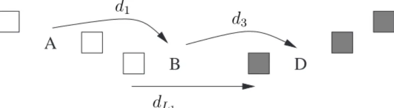
A B C D d1 d3 d2
Figure 6: A 3D example from O’Boyle and St¨ohr.
Consider now an example of O’Boyle and St¨ohr [13], Figure6. Only one barrier is needed in the innermost loop L1for the internal (loop-carried) dependence d2 = (C, B). The rightmost placement
places a barrier just before the ENDDO of L1. This cuts the outgoing dependence d3 = (B, D). The incoming dependence d1 = (A, C) can also be cut by an optimal placement in the innermost
loop, with a (rightmost) barrier before B – so d1 is (A, B) now – but in this case, d3 is not cut.
Therefore, weaving the innermost loop leads to the NCIF in Figure7.
A D B d1 d3 dL1
Figure 7: Woven NCIF for the NCIF of Figure 6.
Now, the innermost loop L2 has 2 internal dependences, dL1 and d3, and only one barrier is needed. The incoming dependence d1 cannot be cut by an optimal placement (if a barrier cuts d1,
it cannot cut d3). Thus, weaving L2 leads to the simple CIF in Figure8. Two barriers are needed, one before the tail of d2, i.e., just before the DO of the second loop, and one before the tail of dL2. This second barrier is interpreted as the rightmost placement for L2, i.e., a barrier just before the
tail of dL1. This one again is interpreted as the rightmost placement for L1, i.e., a barrier just before the ENDDO of this loop. The final barrier placement, in Figure6, has one barrier at depth 3 and one barrier at depth 1. This solution is optimal: it has lower tree cost than the alternative, barriers before B (depth 3) and D (depth 2).
A d
L2
d1
Figure 8: Woven CIF for the NCIF of Figure7.