HAL Id: tel-02408144
https://hal.archives-ouvertes.fr/tel-02408144
Submitted on 12 Dec 2019HAL is a multi-disciplinary open access archive for the deposit and dissemination of sci-entific research documents, whether they are pub-lished or not. The documents may come from teaching and research institutions in France or abroad, or from public or private research centers.
L’archive ouverte pluridisciplinaire HAL, est destinée au dépôt et à la diffusion de documents scientifiques de niveau recherche, publiés ou non, émanant des établissements d’enseignement et de recherche français ou étrangers, des laboratoires publics ou privés.
Defects on the Laminar-Turbulent Transition of a
Boundary Layer with Wall Suction
Jeanne Methel
To cite this version:
Jeanne Methel. An Experimental Investigation of the Effects of Surface Defects on the Laminar-Turbulent Transition of a Boundary Layer with Wall Suction. Fluids mechanics [physics.class-ph]. Institut Supérieur de l’Aéronautique et de l’Espace (ISAE-SUPAERO) Université de Toulouse, 2019. English. �tel-02408144�
THÈSE
THÈSE
En vue de l’obtention duDoctorat de l’Université de Toulouse
Délivré par : l’Institut Supérieur de l’Aéronautique et de l’Espace (ISAE-SUPAERO) Spécialité : Dynamique des Fluides
Présentée et soutenue le 04/11/2019 par :
Cam-Tu Jeanne METHEL
An Experimental Investigation of the Effects of Surface Defects on the Laminar-Turbulent Transition of a Boundary Layer with Wall Suction
JURY
Jens H. M. FRANSSON Rapporteur
Jacques BORÉE Rapporteur
Christophe AIRIAU Président, Examinateur
Laurent MALARD Examinateur
Grégoire CASALIS Directeur de thèse
Maxime FORTE Codirecteur de thèse
École doctorale :
ED MEGEP (ED468)
Unité de Recherche :
ONERA/DMPE
Date :
Dissertation submitted for the degree of
Doctor at the University of Toulouse
Awarded by: l’Institut Supérieur de l’Aéronautique et de l’Espace (ISAE-SUPAERO) Specialty: Fluid Dynamics
Defended on November 4th, 2019 by:
Cam-Tu Jeanne METHEL
An Experimental Investigation of the Effects of Surface Defects on the Laminar-Turbulent Transition of a Boundary Layer with Wall Suction
Date: November 4th, 2019
To cite this dissertation:
Jeanne Methel. An Experimental Investigation of the Effects of Surface Defects on the Laminar-Turbulent Transition of a Boundary Layer with Wall Suction. ISAE-SUPAERO, Université de Toulouse, 2019.
BibTEX entry:
@phdthesis { methel2019dissertation , author ={ Methel , Jeanne },
title ={ An Experimental Investigation of the Effects of Surface Defects on the Laminar - Turbulent Transition of a Boundary Layer with Wall Suction },
school ={ ISAE - SUPAERO , Universit \’{e} de Toulouse }, year ={2019} ,
address ={ Toulouse , France } }
An Experimental Investigation of the Effects of Surface Defects on the Laminar-Turbulent Transition of a Boundary Layer with Wall Suction
by
Cam-Tu Jeanne Methel PhD dissertation defended on
November 4th, 2019.
ISAE-SUPAERO, Université de Toulouse, France.
Abstract
The projected increase in air traffic volume has led to a renewed interest in drag reduction research to reduce aviation’s environmental impact. One solution is wall suction, which can effectively postpone the laminar-turbulent transition of a boundary layer developing over an aircraft’s wetted area. Since a boundary layer in the laminar regime has lower skin-friction coefficient than in the turbulent regime, a delayed transition results in lower drag and reduced fuel consumption. However, implementing a suction system is likely to introduce surface defects, especially at the junction between the suction and solid panels. Additionally, surface defects generally tend to promote transition, and could therefore cancel any drag reduction achieved by wall suction.
The aim for the present research is to study the combined effects of surface defects and wall suction on the transition of a Blasius boundary layer in two-dimensional incompressible flow. First, an experimental protocol was developed and implemented to verify the quality of the aerodynamic conditions in the test facility, and establish a reference for the smooth case with different suction distributions. As expected, wall suction always delayed transition, compared to the configuration without suction, and had varying effectiveness depending on the suction configuration. Concurrently, porous panels without suction were found to destabilize the boundary layer. Subsequently, three types of surface defects (wires, forward-facing steps and gaps) were tested with wall suction. No significant differences between configurations with and without suction were observed. In particular, the critical defect dimensions (height and/or width), for which transition occurs at the defect location, were identical regardless of the suction configuration. For subcritical defects (where transition is not triggered immediately) however, wall suction could still delay transition, albeit less effectively than in the smooth case.
Keywords: Boundary layer, Laminar-turbulent transition, Laminar Flow Control, Tollmien-Schlichting instabilities, Wall Suction, Surface defects.
Acknowledgments
If there is one phrase that comes to mind for these acknowledgments, it is “It takes a village
to raise a child”. In the present case, I can honestly say that it took a whole department (and
even more, to be honest!) to “raise” me into a researcher. I would therefore like to single out the people who truly made a contribution during my three years at ONERA.
At the tip of the iceberg, I would first like to extend my thanks to the two reviewers, Dr. Jens Fransson and Dr. Jacques Borée who took the time to read this dissertation, and thanks to whom the present work greatly benefited. Thank you also to Dr. Christophe Airiau and Dr. Laurent Malard for being committee members, and for their interest in this work.
J’aimerais aussi saluer Pierre Millan et Estelle Piot pour m’avoir accueilli au sein de leur département DMPE et unité ITAC, respectivement, et de m’avoir laissé mener mes expériences quelque peu sonores, au détriment de toute la productivité du côté sud-ouest du bâtiment. Je leur suis aussi reconnaissante de m’avoir permis de participer à des congrès ainsi que de ne m’avoir jamais fait payer la facture d’électricité de ma soufflerie.
Ensuite, j’aimerais remercier mon directeur de thèse Grégoire Casalis qui, en dépit de la “distance” (nouveau portail oblige), a su être présent aux moments clefs de cette thèse pour me faire part de son expérience et de ses bons conseils. Sa pédagogie n’a jamais fait faute et a toujours amené beaucoup de nuance à ces travaux.
À Maxime Forte, my boss et co-directeur de thèse, qui malgré le nombre incalculable de fois où il m’aura “viré”, je lui suis inexprimablement reconnaissante du temps, lui aussi incalculable, qu’il aura passé à m’écouter, à m’encourager, à me guider et à se salir les mains sur ma manip. Sa grande rigueur et sa passion scientifique (“Pendant que j’étais en train de faire la route cet après midi, je me suis demandé...”) m’auront orienté tout le long de cette thèse et je serai éternellement reconnaissante d’avoir eu la chance de travailler en sa compagnie. Grâce à lui, j’aurai vu la plus grande soufflerie du monde, un magicien fou, un lampadaire de (trop) près et son adorable petite fille qui voulait jouer avec moi au Jardin des Plantes lors des moments les plus tendus de la rédaction. Avec tout le respect et l’affection imaginables: MERCI MAX!
À Olivier Vermeersch, mon encadrant “théorie” mais pas “théorique”, qui lui aussi m’aura toujours gardé sa porte ouverte, quel que soit le niveau de...“confusion” de mes questions, je le remercie de son soutien constant et de ses encouragements précieux. Sa contribution scientifique et ses relectures éclairs auront été d’une valeur inestimable. Je lui exprime aussi ma sincère gratitude pour toutes les opportunités extra-thèse qu’il m’aura permis ainsi que ses bons conseils pour l’après-thèse.
À Fabien Méry, mon encadrant “honorifique” qui malgré sa participation entièrement bénév-ole à cette thèse m’aura lui aussi accordé un nombre d’heures inimaginables (et “non-pointables”, je suis sûre), je le remercie sincèrement. Sans l’ombre d’un doute, son enthousiasme, ses encour-agements et même son humour sans merci, auront grandement contribué à cette thèse.
Je tiens ensuite à exprimer ma gratitude à toutes les personnes qui ont formé le support “technique” et sans qui cette thèse n’aurait pas abouti. Un grand merci à Valérie Duplessis pour son soutien et son amitié ainsi qu’à Corinne Plantade pour son aide au quotidien. Je remercie
aussi Nicolas Fasano pour ses bons conseils, sa pédagogie et son potager devant l’atelier (qui, à un moment, était bien la seule chose qui “marchait” dans ma thèse) ainsi que Thomas Batmalle pour son assistance éclectique, allant de coder du LabVIEW à préparer du foie gras pour le repas de Noël.
Je suis aussi reconnaissante envers Floris Bigot pour sa réactivité et son aide dans les mo-ments tendus ainsi qu’à Michel Schiavi et Francis Bisme pour leur contribution lors du montage initial de la manip. Marie-Louise Moretto ne m’aura pas seulement aidé aux achats mais elle m’a aussi longuement écouté lors de mes (inombrables) soucis techniques, je l’en remercie. Un grand merci à Patrick Nicouleau et à Philippe Brunet d’avoir redémarré ma soufflerie quand tous les plombs sautaient, ainsi qu’à Jean-Paul Nigoul qui m’a non seulement aidé au service impression mais qui m’a aussi ramené des urgences lorsque je m’étais déboîtée la cheville. Et j’aimerais aussi remercier très chaleureusement Marie Sanchez, qui ne s’est pas seulement oc-cupée des locaux dans lesquels je travaillais, mais qui a aussi su égayer mes matins avec son affection et son espièglerie.
Je remercie aussi chaleureusement tous les “permanents” (quel étrange concept!) du DMPE Toulouse, du Fauga-Mauzac et même certains de Paris pour leur contribution technique ou morale à cette thèse et qui, en tant qu’ensemble, auront fait office d’énorme canard en plas-tique. Dans l’unité ITAC en particulier, je tiens à reconnaître Hugues Deniau pour sa gentil-lesse et toutes nos supers conversations (Trumpiiiie), Delphine Sebbane pour son aide toujours disponible, Jean-Philippe Brazier d’avoir été à l’écoute et Gréguy Delattre pour l’intérêt qu’il aura porté à cette thèse. Un merci spécial à Lucas Pascal avec qui on a bien rigolé (snowballs) et qui m’aura chaleureusement invité à partager de supers moments avec ses chouettes colocs (Alix, Élise, Célie, Alexia, Adèle, Max) que je remercie aussi.
Hors ITAC, je remercie Christophe Corato, Jouke Hijlkema, François Chedevergne, Julien Troyes, Jean-Michel Lamet, Lionel Tesse, Pierre Berthoumieu, Pierre Gajan, Hervé Bézard, Hélène Gaible, Geoffroy Illac, Francis Micheli, Olivier Rouzaud, Guillaume Puigt, Frédéric Bigot, Cécile Ghouila Houri et Pierre Moré de Lille, Michaël Ridel et François Monsieur 50 Hz du DEMR, l’équipe de l’atelier du DMPE/SRE, l’équipe de S2 de Modane et de F2 du Fauga: chacun a participé de près ou de loin à faire de cette thèse un moment agréable et mémorable. En toute subjectivité, je tiens aussi à identifier et exprimer ma sincère reconnaissance aux permanents DMPE ayant le meilleur passe-temps du monde: Olivier Léon, le bloc-eur à la pince d’acier, Claire Laurent, la grimpeuse aux petites filles qui chatouillent sans pitié et Olivier Dessornes, le Bleausard qui m’aura fait découvrir LE bloc et le concept de “la collante”. Rock on!!
Vient ensuite la tâche délicate de “catégoriser” les doctorants: je m’excuse d’avance de toute “erreur”. Je remercie tout d’abord mes co-doctorants de promotion: Émilie Jahanpour mon unique co-doctorantE toujours souriante, Thibault Xavier mon camarade de spectacles, Jean-François Poustis mon co-martyr des JDD, Baptiste Thoraval mon compère de cinéma, Anthony Desclaux mon comparse de manips récalcitrantes, Quentin Levard un des clandestins du Fauga avec qui on aura toujours bien rigolé aux repas de Noël, Loic Van Ghèle le cuisinier aux mille talents et Jean-Etienne Durand l’autre clandestin que j’aurais plus souvent vu en ville qu’à l’ONERA. Malgré les campus et les étages différents, on aura quand même souvent trouvé l’occasion de passer de bons moments ensemble, tant au labo qu’à l’extérieur, et je vous en remercie!
Je remercie aussi les anciens, François N., François L., Jéré Derré, Maxime B., Stéphanie B. et Natacha S. pour leurs conseils (que je ne comprends que maintenant hélas!) ainsi que les générations suivantes (Julien S.-J., Loïc A., Damien T., Gaétan C., Eric N.-V., Adèle V., Victor L., Ludovic T., Yann M., Pierre S., Loris C., Rémi H., Tanguy T., Romain P., Adrian C.-G., Beatrice F., Arthur C., Nadine B., Pierre V.-M. et Valentin M.) et les post-doctorants (Christian
iii C., Romain F., Alexis M., Hala G.) pour la bonne ambiance et les vendredi matins gourmands et salutaires! Un petit clin d’œil fraternel à mon “little brother” Félix Ducaffy et mes “baby brothers” de thèse Adrien Rouviere et Thomas Jaroslawski: on ne choisit pas sa famille, même de thèse, alors FAÎTES DU BRUIT!! (I mean it, literally.)
Et puis, il y en a forcément quelques uns avec qui on a des atomes plus crochus. À mon co-bureau Sylvain Morilhat, le marin féru de littérature et de cuisine (la galette qui roule, qui roule...), avec qui on aura passé de nombreuses soirées à discuter et qui n’aura jamais hésité à prendre le temps de m’expliquer moultes sujets, un grand merci. J’exprime aussi toute ma gratitude à Rémi Roncen, le Wizard (or is it Warlock?) de l’humour tordant qui m’aura apporté son soutien perpétuel par ses encouragements, sa bonne humeur et d’inombrables pauses déjeuner/goûter/thé/café. Merci à Loïc Jecker, l’éleveur de levures variées, pour toutes nos conversations stimulantes qui auront été des coupures appréciées, surtout en troisième année. Je remercie aussi Lola Rousseau de m’avoir fait découvrir les pâtes à LA carbonara et pour les bons moments en randonnée, malgré des bovins belligérants. E Lorenzo Lanzillotta, ti ringrazio profondamente per avere aperto la porta della tua casa e delle tue montagne con tanta generosità e per essere un così grandissimo amico. (Che vergogna... Scusa per gli errori e per fortuna, non senti gli accenti tonici!)
Durant la thèse, j’ai aussi eu la chance de profiter de mes chères Pyrénées (ne le dîtes pas à Max, il risquerait de me virer) et je remercie donc Christophe Martin, celui qui m’aura initié à l’alpinisme, ainsi que Thibault Pouiller et Cindy Sauvaigo, qui auront partagé la même corde que moi, pour ces supers moments en montagne. Je remercie aussi affectueusement ma grande amie Chantal Sibrac de m’avoir accueilli si gentiment au sein de sa famille et pour tous nos moments de grimpe (dedans, dehors, sur spits et sur friends...) qui ont été essentiels à ma santé mentale.
Et finalement, je tiens aussi à exprimer ma reconnaissante à toutes les personnes “d’avant la thèse” qui m’ont apporté leur soutien et leur amitié durant la thèse. Merci à Charlotte Cobb, ma plus ancienne amie qui aura toujours été là pour moi, à Julia Experton qui aura été une amie fidèle et à François Sanson pour sa confiance et son amitié.
I would also like to thank my friends peppered across different countries: Nicoletta Fala, whose close contact and constant friendship evaporated the kilometers (miles?) and whose support was indispensable, Adam Ouammou and Kimranpal Mann with whom I had some of the best culinary adventures and who shared their hospitality and affection with me so generously, as well as Jas’Minique Potter, Amanda Brock, Nyansafo Aye-Addo, Theresa d’Aquila and Bryce Heckaman who have maintained their friendship despite the distance. Thank you also to Dr. Gregory Blaisdell for his help in getting admission to this PhD program and in some of my other endeavors. I also want to express my sincere gratitude to Philip and Christy Owen, who have allowed me a little spot in their wonderful family and who have supported me through all of my graduate degrees.
Je tiens aussi à remercier Florian Monteghetti pour son “apparition” durant la thèse et qui m’aura apporté son soutien, son affection et sa rigueur pendant les moments les plus difficiles de la thèse. Merci et vivement la suite!
Et bien sûr, last but most definitely not least, je remercie de tout mon coeur ma famille: mon papa, ma maman, my second dad et Michelle dont la confiance et l’affection inconditionnelles m’ont toujours guidé et encouragé.
La technique résout les problèmes et apporte des satisfactions mais elle n’est qu’un moyen et reste pauvre si on la sépare de l’esprit qui la guide.
Contents
Table of Contents ix
List of Figures xiii
List of Tables xv
Acronyms xvii
Notation xix
Introduction xxi
I Literature Review 1
1 Laminar-Turbulent Transition of a Boundary Layer 3
1.1 Boundary layer theory . . . 3
1.1.1 Prandtl boundary layer equations . . . 4
1.1.2 Boundary layer parameters . . . 6
1.1.3 The Blasius solution for a laminar boundary layer . . . 8
1.2 Modeling and prediction of the laminar-turbulent transition . . . 9
1.2.1 Path to transition . . . 11
1.2.2 Small perturbation theory and the Orr-Sommerfeld equation . . . 12
1.2.3 Predicting transition location: the eN method . . . 14
1.2.4 Numerical tools . . . 16
2 Laminar Flow Control Using Wall Suction 17 2.1 Laminar flow technologies . . . 17
2.2 Boundary layer stabilization using wall suction . . . 18
2.3 Design parameters for wall suction applications . . . 20
2.4 Current challenges to the widespread implementation of HLFC . . . 21
2.5 Effect of a porous wall without suction on transition . . . 22
2.5.1 Definitions . . . 22
2.5.2 Porous wall effect on boundary layer properties . . . 23
2.5.3 Attempts at using a porous wall for Laminar Flow Control purposes . . . 24
3 Effects of Two-Dimensional Surface Defects on Transition 27 3.1 Transition mechanisms in the presence of 2D surface defects . . . 27
3.1.1 General effects of surface defects on transition mechanisms . . . 28
3.1.2 Identification of the parameters of interest . . . 29 vii
3.2 Flow geometry and resulting effects of 2D surface defects on transition . . . 31
3.2.1 Steps: Forward-Facing Steps (FFS) and Backward-Facing Steps (BFS) . . 31
3.2.2 Positive surface defects: wires and humps . . . 31
3.2.3 Negative surface defects: gaps . . . 32
3.3 Transition prediction for flows with 2D surface defects . . . 35
3.3.1 Empirical criteria . . . 35
3.3.2 N method . . . 36
3.3.3 Numerical simulation approach . . . 39
3.4 Combined effect of steps and wall suction . . . 39
II Fundamentals for a Laminar-Turbulent Transition Investigation 41 4 Experimental Protocol for a Laminar-Turbulent Transition Study 43 4.1 Presentation of the experimental facility . . . 43
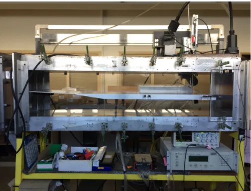
4.1.1 TRIN 2 subsonic wind tunnel . . . 43
4.1.2 Flat plate model . . . 45
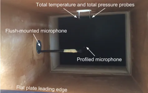
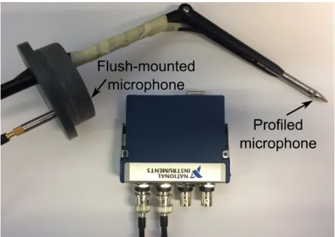
4.1.3 Instrumentation and data acquisition systems . . . 45
4.2 Validation of the experimental protocol . . . 49
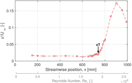
4.2.1 Test section flow characterization . . . 49
4.2.2 Baseline flat plate measurements . . . 51
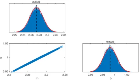
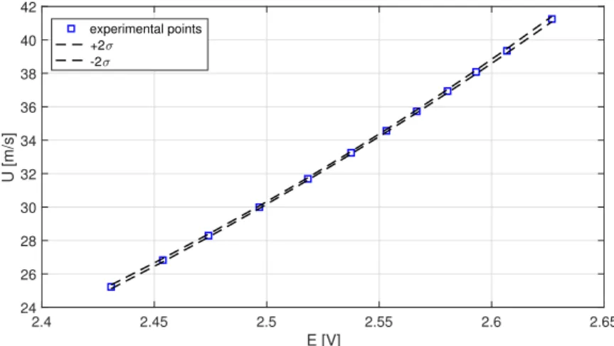
4.3 Measurement uncertainty analysis . . . 55
4.3.1 Boundary layer profiles . . . 56
4.3.2 Transition position . . . 60
4.3.3 Pressure coefficient . . . 60
III Experimental Investigations with a Wall Suction System 65 5 Wall Impedance and Suction Effects on Laminar-Turbulent Transition 67 5.1 Wall suction parameters and suction configurations . . . 67
5.1.1 Suction panel geometric parameters . . . 67
5.1.2 Summary of the reference 1995 study . . . 68
5.2 Effects of a porous wall without suction . . . 70
5.2.1 Experimental characterization . . . 70
5.2.2 Numerical analysis . . . 75
5.3 Effect of wall suction and suction distribution . . . 79
6 Combined Effects of Wires and Wall Suction 89 6.1 Geometric characteristics of the wires . . . 89
6.2 Transition location and mean flow . . . 90
6.3 Spectral and numerical stability analyses . . . 95
7 Combined Effects of Forward-Facing Steps and Wall Suction 99 7.1 Geometric characteristics of the FFS . . . 99
7.2 Transition location and mean flow . . . 100
7.3 Unsteady data analysis . . . 106
Contents ix
8 Combined Effects of Gaps and Wall Suction 117
8.1 Geometric characteristics of the gaps . . . 117
8.2 Transition location and mean flow . . . 118
8.3 Unsteady data analysis . . . 123
8.4 Numerical analysis and comparison with an existing model . . . 131
9 Comparison of the effects of all surface defects combined with suction 135 9.1 Transition criteria . . . 135
9.2 Transition mechanisms . . . 136
Conclusion 139 IV Appendices 143 A Flat plate leading edge geometry 145 B Wall suction uniformity across chambers 147 B.1 Suction uniformity tests for each suction chamber . . . 147
B.2 Suction uniformity tests for the suction configurations used in present study . . . 151
V French summary / Résumé 153
List of Figures
1.1 Schematic representation of boundary layer evolution . . . 4
1.2 Displacement thickness ”1 . . . 7
1.3 Momentum thickness ◊ . . . . 7
1.4 Schematic of boundary layer profiles with varying shape factors . . . 8
1.5 Flow visualization of TS waves . . . 12
1.6 Boundary layer parameter evolution during transition . . . 13
1.7 Stability diagram and N factor evolution for a wave at frequency f1 . . . 15
2.1 The different approaches to maintain laminar flow over an airfoi . . . 18
2.2 Mean velocity and TS profiles with and without suction . . . 19
2.3 Flow visualization of horseshoe vortices around perforation with suction . . . 21
2.4 Inside the leading edge of the DLR Do 228 for HLFC flight test . . . 22
2.5 Schematic TS instability interacting with porous wall . . . 23
2.6 Neutral stability curves for various wall permeability . . . 25
3.1 Effect of freestream turbulence and wires on transition Reynolds number . . . 30
3.2 Types of two-dimensional surface defects presented in this document . . . 31
3.3 Flow geometry around BFS and FFS from Perraud and Séraudie 2000 . . . 32
3.4 Summary of the experimental data of gaps on transition at ONERA . . . 34
3.5 Graphical summary of the N method and sample results . . . 37
3.6 Experimental N correlations for BFS and FFS . . . 38
3.7 Numerical N correlations with respect to relative height for FFS and BFS . . . 38
4.1 CAD overview of the TRIN 2 subsonic wind tunnel (Susie) . . . 44
4.2 Photograph of the test section with flat plate . . . 44
4.3 Numerically optimized leading edge shape . . . 46
4.4 General layout of the flat plate detailing the suction region . . . 46
4.5 PSD(u’) showing test facility ground interference . . . 47
4.6 Schematic representation of the y correction . . . 48
4.7 Streamwise fluctuations for transition position on solid wall panel . . . 48
4.8 Test section flow characterization . . . 50
4.9 Microphone set-up at the test section entrance for acoustic characterization . . . 50
4.10 Acoustic data acquisition system with side view of the profiled microphone . . . 51
4.11 Overall SPL evolution over range of operating unit Reynolds numbers . . . 51
4.12 Acoustic characterization at varying unit Reynolds numbers . . . 52
4.13 Nominal pressure coefficient distribution along the flat plate . . . 53
4.14 Integral values of the boundary for the solid wall (no porosity) flat plate . . . 53
4.15 Two-dimensional transition position for the solid wall panel . . . 54
4.16 Identification of ≥600 Hz TS profile . . . 54 xi
4.17 N-factor evolution for Blasius flow at operating Reynolds number . . . 55
4.18 Output from statistical calibration for sample test . . . 57
4.19 Calibration curve uncertainties for sample test . . . 58
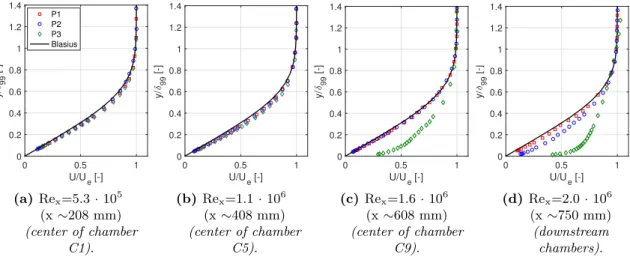
4.20 Normalized mean velocity profile for sample test with uncertainties . . . 61
4.21 ormalized mean velocity profile for all tests with uncertainties . . . 62
4.22 Streamwise evolution of numerical TS profiles . . . 62
4.23 Streamwise velocity fluctuations for various constant height hotwire traverses . . 63
4.24 Nominal pressure coefficient distribution with uncertainties . . . 63
5.1 Amplitude evolution of instabilities for suction cases from Casalis et al. 1996 . . 69
5.2 Streamwise evolution of mean velocity profiles for all panels without suction . . . 71
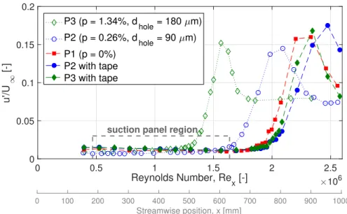
5.3 Two-dimensional transition position for all panels . . . 71
5.4 Streamwise velocity fluctuations for all panel configurations without suction . . . 72
5.5 PSD(u’) at a position upstream of the transition location . . . 73
5.6 PSD(u’) at x ≥508 mm for all panels . . . 73
5.7 Velocity fluctuation profiles for all panels without suction . . . 74
5.8 Streamwise evolution of the u’ profile maximum amplitude for all panels . . . 75
5.9 Neutral stability curve for real-only impedance . . . 76
5.10 Neutral stability curve of imaginary-only impedance . . . 77
5.11 Neutral stability curves based on experimental impedance values . . . 78
5.12 N factor envelope curves from numerical analysis with impedance . . . 78
5.13 Isocontours of –i from linear stability theory with and without suction . . . 79
5.14 Boundary layer profiles for all suction configurations (panel P2) . . . 80
5.15 Experimental and numerical boundary layer profiles with suction . . . 81
5.16 Streamwise velocity fluctuations for all suction configurations . . . 81
5.17 Streamwise evolution of experimentally-evaluated shape factor H . . . 82
5.18 Streamwise velocity fluctuations for full suction for panels P2 and P3 . . . 83
5.19 Effect of suction on u’ profile evolution for panel P2 . . . 84
5.20 Effect of suction on u’ profile evolution for panel P3 . . . 85
5.21 TS-profile maximum amplitude evolution for panels P2 and P3 . . . 86
5.22 Maximum N factor envelope curve for all suction configurations . . . 87
5.23 Wall suction distribution effect on the instability at a particular frequency . . . . 88
6.1 Overview of the flat plate with the different wire locations and dimensions . . . . 90
6.2 Streamwise velocity fluctuations for different wires and suction configurations . . 92
6.3 Boundary layer profiles 1 mm downstream of the wire . . . 93
6.4 Transition parameters variation with respect to relative wire height . . . 94
6.5 PSD(u’) upstream of WIR-300µm-640 for all suction configurations . . . 96
6.6 PSD(u’) just upstream of respective RexT for different wires . . . 97
6.7 Neutral stability curves for profiles with and without inflection point . . . 98
7.1 Overview of the flat plate with an FFS . . . 100
7.2 Streamwise velocity fluctuations for different FFS relative heights . . . 102
7.3 Mean velocity profiles in the FFS region for h/”1 ≥0.6 . . . 103
7.4 Mean velocity profiles in the FFS region for h/”1 ≥1.4 (crit.) . . . 103
7.5 Mean velocity profile in the FFS region for different FFS height . . . 104
7.6 Transition position summary for all tested FFS . . . 105
7.7 PSD(u’) upstream and downstream of the subcritical FFS . . . 106
7.8 PSD(u’) at the transition Reynolds number for the subcritical FFS . . . 107
List of Figures xiii
7.10 PSD(u’) at the transition Reynolds number for C1/0.400 . . . 108
7.11 Velocity fluctuation profiles around the FFS for no suction. . . 109
7.12 Velocity fluctuation profiles upstream and downstream of the FFS for C1/0.400 . 110 7.13 Velocity fluctuation profiles around the FFS for full suction . . . 111
7.14 Evolution of TS profiles for different FFS heights and suction configurations . . . 111
7.15 Evolution of the TS profiles maxima for different suction configurations . . . 114
7.16 N evaluation for the solid panel with FFS . . . 115
7.17 N as a function of h/”1 . . . 115
7.18 All suction configurations with FFS compared with other N data sets . . . 115
8.1 Overview of the flat plate with the two gap inserts . . . 118
8.2 Streamwise velocity fluctuations for different gaps (xGAP = 640 mm) . . . 120
8.3 Streamwise velocity fluctuations for different gaps (xGAP = 360 mm) . . . 121
8.4 Evolution of the mean velocity profiles over critical gap . . . 122
8.5 RexT as a function of b/h . . . 123
8.6 xT vs different gap parameters . . . 124
8.7 Comparison with experimental data from previous ONERA studies . . . 125
8.8 PSD(u’) upstream (a) and downstream (b) of a subcritical gap . . . 125
8.9 PSD(u’) at the transition position for subcritical gap (xGAP = 640 mm) . . . 126
8.10 PSD(u’) upstream (a) and downstream (b) of gaps for C1/0.400 . . . 126
8.11 PSD(u’) at the transition position of different gaps for C1/0.400 . . . 127
8.12 PSD(u’) downstream of critical GAP-1200µm-18mm . . . 128
8.13 Evolution of u’ profiles for GAP-1200µm-8mm (xGAP = 640 mm) . . . 129
8.14 Evolution of u’ profiles for GAP-1200µm-2.4mm (xGAP = 360 mm) . . . 130
8.15 Evolution of u’ profiles for critical GAP-1200µm-20mm (xGAP = 640 mm) . . . . 130
8.16 Evolution of u’ profiles for critical GAP-1200µm-18mm (xGAP = 360 mm) . . . . 131
8.17 TS profiles maximum for a subcritical and critical gap (xGAP = 640 mm) . . . . 131
8.18 TS profiles maximum for a subcritical and critical gap (xGAP = 360 mm) . . . . 132
8.19 Comparison of the u’ profile maxima for gaps at both locations for C1/0.400 . . 132
8.20 N values evaluated for all suction configurations and gap dimensions . . . 133
8.21 All suction configurations with gaps compared with a N model . . . 133
9.1 Comparison of the xT parameter for all wires and FFS (without detail) . . . . 136
9.2 Comparison of the xT parameter for all wires and FFS (with details) . . . 136
9.3 PSD(u’) at RexT for selected subcritical defects for full suction . . . 137
9.4 PSD(u’) at RexT for selected critical defects for full suction . . . 138
B.1 Suction uniformity inside chamber C1 . . . 148
B.2 Suction uniformity inside chamber C3 . . . 149
List of Tables
1.1 Blasius solution for laminar flow on a flat plate with zero pressure gradient . . . 10 3.1 Summary the flow geometries around cavities from Sinha et al. 1982 . . . 34 4.1 Instrument uncertainties as provided by manufacturer . . . 59 4.2 Hotwire calibration data sets and related uncertainty parameters . . . 60 5.1 Panel parameters . . . 68 5.2 Experimental xT for all configurations in Juillen et al. 1995 . . . 69
5.3 Numerical and experimental transition position for all panels without suction . . 79 5.4 Transition positions for all suction cases and all suction panels . . . 82 5.5 Transition positions and N factors for all suction configurations (panel P2) . . . 85 6.1 Summary of the wire (WIR) geometry and position. . . 90 6.2 Local boundary layer thickness (numerical value) at surface defect location . . . 91 6.3 RexT for panel P1 (p = 0%) . . . 95 6.4 RexT for suction panel P2 (p = 0.26%) . . . 95 6.5 RexTfor suction panel P3 (p = 1.34%) . . . 95 7.1 Relative heights for FFS at streamwise position xFFS = 430 mm . . . 100 7.2 Relative heights for FFS at streamwise position xFFS = 640 mm . . . 100 7.3 Relative heights for FFS and panel P1. . . 101 8.1 All tested gap dimensions for xGAP = 640 mm . . . 118 8.2 All tested gap dimensions for xGAP = 360 mm . . . 119 A.1 Leading edge coordinates on the lower side . . . 145 A.2 Leading edge coordinates on the upper side . . . 146 B.1 Suction chamber pressure drop measurements over chamber C1 . . . 147 B.2 Suction chamber pressure drop measurements over chamber C2 . . . 148 B.3 Suction chamber pressure drop measurements over chamber C3 . . . 148 B.4 Suction chamber pressure drop measurements over chamber C4 . . . 149 B.5 Suction chamber pressure drop measurements over chamber C6 . . . 149 B.6 Suction chamber pressure drop measurements over chamber C7 . . . 150 B.7 Suction chamber pressure drop measurements over chamber C8 . . . 150 B.8 Suction chamber pressure drop measurements over chamber C9 . . . 150
Acronyms
BFS Backward-Facing Step CAD Computer Aided Design FFS Forward-Facing Step
HLFC Hybrid Laminar Flow Control LFC Laminar Flow Control
LST Linear Stability Theory NLF Natural Laminar Flow PSD Power Spectral Density rms room mean square rpm revolutions per minute TS Tollmien Schlichting
Notation
Greek letters
– Wave number (complex variable) ”1 Displacement thickness
”99 Boundary layer thickness at 0.99ue
◊ Momentum thickness µ Dynamic viscosity ‹ Kinematic viscosity fl Density ‡ Standard deviation Ê Angular frequency
Roman letters
Cp Pressure coefficient d Suction hole diameterH Shape factor
h Wire diameter
N Amplification factor
p Porosity
Re Reynolds number
U Streamwise (x) component of velocity
uÕ Streamwise (x) component of velocity fluctuation x Streamwise coordinate
y Normal coordinate to the flate plate wall z Spanwise coordinate
Subscripts
ΠFreestream
atm atmospheric
dyn Dynamic
e Boundary layer edge
ref Reference
SD Surface defect xT, T Transition location
Introduction
In the present dissertation, the effects of surface defects on the laminar-turbulent transition of a boundary layer undergoing wall suction are experimentally investigated and analyzed. The purpose of this study is to: provide insight on the physics of the competing effects of the stabilizing wall suction and generally destabilizing surface defects on boundary layer stability; as well as offer validation data for numerical models. The current lack of transition prediction models that can account for this combined effect is one of the remaining obstacles preventing the more widespread implementation of wall suction as a drag reduction technology on conventional aircraft.
This introduction is divided in three parts. First, a general overview of the individual effects of wall suction and surface defects on boundary layer transition is briefly discussed, followed next by a presentation of the scope and objectives of the present investigation. Finally, a detailed outline of the present document is provided.
Background
The projected increase in air traffic volume, coupled with the need to reduce air pollution for environmental sustainability, has led to a renewed interest in laminar flow research to reduce aviation’s fuel consumption. In particular, the objective of any laminar flow technology is to reduce skin friction drag, which can represent up to 40% of the total drag for a typical civil transport aircraft (Marec 2001).
Boundary Layer Transition
The concept of a boundary layer for flows at high Reynolds numbers was first introduced and modeled by Prandtl 1904. In the presence of relative motion between a body and a surrounding flow, the boundary layer region, located close to the body’s wall, acts as an interface between the freestream region, where flow can be assumed to be inviscid, and the zero velocity (no-slip) boundary condition at the wall. High shear stresses are consequently present because of the large velocity gradients that occur across this thin region. Additionally, the boundary layer is characterized by the presence of viscous forces that are of the same order as inertial forces.
In the remainder of the present document, two-dimensional flow will be assumed unless oth-erwise stated. Past the stagnation point, the boundary layer first develops in the laminar regime, then goes through a more or less extended transition region, and finally settles into the fully turbulent regime. In a low freestream turbulence flow, freestream perturbations enter the bound-ary layer through the receptivity phase. The main process that then drives the boundbound-ary layer to transition is the linear amplification of primary modes (also known as Tollmien-Schlichting instabilities) up to a certain threshold amplitude, past which secondary and other non-linear instabilities quickly amplify and lead to the breakdown to turbulence.
The linear amplification stage can effectively be reproduced numerically using Linear Sta-bility Theory (LST). Although mode amplification is exponential, the term "linear" refers to the assumptions that each mode is considered to develop itself independently from the others. Based on LST, amplification factors (N factors) are calculated at each frequency of interest. One transition prediction method consists in defining the transition position as the location where a threshold NT factor is reached. This threshold NT can be determined, for example, using
Mack’s relation (Mack 1977), which relates freestream turbulence and NT, or from experimental
data. In general, the efforts to predict transition and increase the extent of laminar flow over an aircraft’s wetted area is driven by the fact that laminar flow has lower skin friction coefficient than turbulent flow (approximately five times lower).
Wall Suction
Two main approaches can be used to maximize the streamwise extent of laminar flow regions and delay laminar-turbulent transition: a passive approach, by using Natural Laminar Flow (NLF) airfoils, and an active approach, by implementing a Laminar Flow Control (LFC) technology. A combination of both techniques, Hybrid Laminar Flow Control (HLFC) can also be implemented. NLF airfoils were successfully developed to achieve larger laminar flow regions, compared to conventional airfoils, over the wings and empennage of commercial aircraft. However, this passive approach consists in optimizing the profile geometry around a single design point and cannot account for different operating conditions. LFC and HLFC technologies, on the other hand, can be adapted during operation so that laminar flow can be achieved over a wider operating range.
One LFC technology is to stabilize the boundary layer using wall suction. Applying wall suction on a boundary layer increases its mean velocity profile curvature (and therefore its stability), and redistributes the disturbance energy closer to the wall where there is higher viscous dissipation. As a result, the growth of boundary layer instabilities is reduced and transition is delayed.
This technique was found to be effective as early as in the 1950s, and numerous test flights and experimental data are available in the literature to attest to this fact (Braslow 1999). Based on various studies, the main design parameters for an independent wall suction system (i.e., excluding any integration issues) that were identified were: suction distribution, panel porosity, panel geometry, and suction velocity.
Numerical studies were also performed to model the effect of wall suction on boundary layer stability. Various numerical approaches demonstrated that suction is most effective when applied upstream of location where the secondary instabilities start to amplify. In attempt to use a "simple" approach, implementation of the eN method on results from HLFC flight tests was also attempted but found to be unsatisfactory because the transition criterion used for this method seemed to vary between test flights and wind tunnel experiment. Based on these studies, wall suction modeling still requires sophisticated numerical tools that cannot easily be incorporated in the aircraft design cycle.
Surface Defects
Current manufacturing techniques do not allow to conceive the implementation of wall suction technology without introducing surface defects (e.g., gaps, forward- and backward-facing steps) at the junction between the porous and solid wall regions. Surface defects generally tend to destabilize the boundary layer either by modifying local receptivity, further amplifying existing instabilities or changing the mean flow stability by introducing inflection points in the mean
xxiii velocity profiles because of the small separation bubbles that can form around a defect. If transition occurs inside the bubble, non-linear effects can also occur inside the separation bubble. A surface defect is termed "critical" by Tani (Tani 1961) when transition occurs immediately downstream of the defect position. In other cases, the transition position can gradually move upstream from the smooth case position, advancing closer to the surface defect location: the defects are subcritical. In these intermediate situations, the main defect parameters that can affect transition are relative geometric parameters (with respect to boundary layer thickness) and pressure gradient. In general, three-dimensional surface defects are found to generate complex three-dimensional flows and significantly amplify instabilities, resulting in much lower critical dimensions with respect to two-dimensional defects.
To model the effect of critical surface defects, the simplest approach first consisted in de-termining empirical criteria based on experimental data. The first criteria mainly depended on freestream properties, and were later refined to include local flow properties. As computational capabilities improved, numerical simulations were performed to study the flow around a surface defect and the resulting effect on boundary layer stability, using for example Direct Numerical Simulations or Linearized Navier-Stokes equations. Although more precise than empirical cri-teria, these types of numerical simulations can be relatively expensive, warranting the use of intermediate approaches.
For the less destabilizing two-dimensional surface defects, an intermediate solution consists in the N approach, based on both numerical and experimental data, and LST calculations. Using this approach, the effect of surface defects on instabilities is modeled as an abrupt shift in N factors, a N, that is determined based on the relative geometric parameters of the defect with respect to local boundary layer thickness. Finally, another way to predict transition with a defect can be by directly modeling a surface imperfection and calculating the resulting flow using Direct Numerical Simulations.
Framework and Objectives
Test flights or wind tunnel experiments have shown that wall suction could effectively stabilize the boundary layer, and thereby delay its laminar-turbulent transition. Numerical transition prediction models were also developed to take into account the stabilizing effect of wall suction on the boundary layer. In parallel, transition criteria were also determined for surface defects such as gaps, forward- and backward-facing steps on "natural" boundary layers, i.e., without suction. However, experimental data are currently not available in the open literature to deter-mine whether or not a boundary layer with suction behaves similarly to one without suction in the presence of a surface defect. As mentioned previously, the relative height of a surface defect with respect to the boundary layer thickness significantly influences transition. Furthermore, wall suction tends to reduce boundary layer thickness. Additional investigations are therefore required to further understand the combined effects of wall suction and surface defects on bound-ary layer stability. With this additional information, transition prediction models can then be modified to account for this interaction more accurately.
The objective of the present study is therefore to perform an experimental characterization of the combined effects of surface defects and wall suction on the laminar-turbulent transition of a boundary layer in two-dimensional incompressible flow. The first objective consisted in de-signing and building an experimental set-up and protocol to perform a transition study. Next, the practical implementation of wall suction along with characterizing the effects of suction cases without surface defects was necessary to establish baseline references. During this process, the non-negligible effect of a porous wall (through which suction is applied) on transition was established, and further investigated both experimentally and numerically. Finally three types
of surface defects (wires, forward-facing steps and gaps) were introduced on the wind tunnel model to investigate their influence on the transition of a boundary layer undergoing wall suc-tion. Experimental characterization and analysis were performed based on measurements of the transition position, mean velocity boundary layer profiles, as well as power spectral densities and profiles of the streamwise velocity fluctuations.
Dissertation Outline
Chapters 1, 2, 3
In the first chapter, a general description of the boundary layer and the laminar-turbulent transition process in an incompressible and low freestream turbulence flow is given. A more in-depth review of the available literature on suction and porous walls effects is then discussed in Chapter 2. Chapter 3 then focuses on the effects of surface defect on transition. The few existing studies (to the author’s knowledge) on the combined effects of surface defects and wall suction are also presented.
Chapter 4
Next, the objective was to develop and validate an experimental protocol to investigate the laminar-turbulent transition of a Blasius boundary layer in a two-dimensional incompressible flow. In this type of low freestream turbulence flow, "natural" transition occurs, resulting from the linear amplification of Tollmien-Schlichting instabilities. The test facility and flat plate model used to obtain a two-dimensional zero-pressure gradient (ZPG) flow are therefore presented in Section 2.1, along with all the necessary instrumentation and data acquisition systems. In Section 2.2, the test section flow is characterized to validate the implementation of the experimental protocol. In particular, baseline flat plate measurements are acquired to verify the presence of a two-dimensional ZPG flow in which transition is the result of the amplification of Tollmien-Schlichting instabilities. Finally, uncertainty analysis is performed in Section 2.3 to complete measurement characterization.
Chapter 5
In the following chapter, the effects of a porous wall and suction on boundary layer transition are investigated using the experimental protocol developed in the previous chapter. Section 5.1 justifies the choice of suction configurations with different spatial distributions that result in various transition locations. The suction panel geometries are therefore presented and the results from a reference study from 1995 are discussed. Based on these findings, suction configurations for the present investigation are selected. In Section 5.2, the effect of a porous panel without suction (i.e., wall admittance) on boundary layer stability is investigated both experimentally and numerically. Finally, Section 5.3 focuses on the effect of wall suction and its spatial distribution on transition. An experimental characterization using mean flow and unsteady data is first performed and then compared to numerical results from Linear Stability Theory (LST).
xxv
Chapters 6, 7, 8
Next, the experimental characterization of the combined effect of wall suction and surface defects on boundary layer transition was performed. The suction configurations defined in the previous chapter were used as a baseline reference over which surface defects could then be introduced. Each chapter corresponds to a type of tested defect: Chapters 6, 7 and 8 focus on the effect of wires, forward-facing steps and gaps, respectively, combined with wall suction. Each chapter begins with a presentation of the defect geometry and position, followed by a discussion on mean flow measurements and transition positions. Unsteady data analysis and LST calculations are then performed to enable comparison with existing numerical models whenever available.
Chapter 9
In the final chapter, the effects on boundary layer stability of all three types of surface defects combined with suction are summarized. Section 9.1 compares the transition criteria of each type of defect while Section 9.2 provides an explanation for these differences based on the varying transition mechanisms involved.
Part I
Chapter 1
Laminar-Turbulent Transition of a
Boundary Layer
Contents
1.1 Boundary layer theory . . . . 3
1.1.1 Prandtl boundary layer equations . . . 4 1.1.2 Boundary layer parameters . . . 6 1.1.3 The Blasius solution for a laminar boundary layer . . . 8
1.2 Modeling and prediction of the laminar-turbulent transition . . . . 9
1.2.1 Path to transition . . . 11 1.2.2 Small perturbation theory and the Orr-Sommerfeld equation . . . 12 1.2.3 Predicting transition location: the eN method . . . 14 1.2.4 Numerical tools . . . 16
T
his chapter first introduces the concept of the boundary layer through Prandtl’s boundarylayer equations, and focuses specifically on the Blasius solution for a laminar boundary layer (Section 1.1). Next, the path to laminar-turbulent transition is presented along with the theoretical and numerical tools that can be used to model and predict transition position (Section 1.2).
1.1 Boundary layer theory
Using potential flow (incompressible and irrotational) theory, in which the effect of viscosity is neglected, the drag generated by the flow around an aerodynamic body cannot be evaluated. In this theory, the fluid offers no resistance to a shape change since there is a perfect slip condition at the body surface. This situation, known as d’Alembert’s paradox, was resolved by the introduction of the concept of a boundary layer by Prandtl 1904. He was able to reconcile the excellent results of potential flow theory, in terms of lift prediction, to the notion of friction drag by recognizing that a flow with large Reynolds numbers around an aerodynamic body could be divided in two regions. One region is the "outer" freestream flow where pressure forces dominate, and potential flow theory is applicable. The second region, close to the body surface, is the "inner" boundary layer flow where friction forces are of the same order as inertial forces.
The boundary layer can be seen as a region of high shear stresses. These stresses are due to the presence of large velocity gradients close to the wall: over a restricted wall-normal distance, flow velocity goes from zero (with respect to the body reference frame) at the wall because of 3
the no-slip condition, up to the freestream velocity. Boundary layer thickness ”, in the wall-normal direction, is then defined as the distance between the wall, and the height at which the streamwise velocity is equal to the local freestream velocity, ue. A thickness ”99 is more commonly used, which represents the distance where u/ue is equal to 0.99.
A boundary layer developing spatially can be divided into three main streamwise regions corresponding to three states: laminar, transitional, and turbulent. A schematic representa-tion of this evolurepresenta-tion over a flat plate is shown in Figure 1.1 along with some representative streamwise velocity distributions. In the freestream region upstream of the flat plate, the ve-locity distribution is assumed to be uniform. Inside the boundary layer, non-uniform veve-locity distributions can be observed. In particular, as the boundary layer transitions from the laminar to the turbulent regime, the velocity gradient close to the wall also increases. Shear stresses are therefore greater in a turbulent boundary layer than in a laminar boundary layer. The main regions of interest in this study are primarily the laminar and transitional regimes, which will be further discussed in the following sections.
Figure 1.1. Schematic representation of boundary layer evolution over a flat plate with zero pressure
gradient. 1.1.1 Prandtl boundary layer equations
In the present development of Prandtl’s boundary layer equations, the flow is assumed to be two-dimensional and incompressible with negligible body forces. Additionally, flow over a flat plate is considered so that the Navier-Stokes equations can be expressed in Cartesian coordinates. The streamwise direction is defined in x, and the wall-normal direction in y. Defining the velocity vector ˛U as
˛
U = (u, v), (1.1)
the continuity and Navier-Stokes equations are written as:
ˆu ˆx + ˆv ˆy =0 (1.2a) ˆu ˆt + u ˆu ˆx+ v ˆu ˆy = ≠ 1 fl ˆP ˆx + ‹ A ˆ2u ˆx2 + ˆ2u ˆy2 B (1.2b) ˆv ˆt + u ˆv ˆx+ v ˆv ˆy = ≠ 1 fl ˆP ˆy + ‹ A ˆ2v ˆx2 + ˆ2v ˆy2 B . (1.2c)
Equation 1.2a is the continuity equation and Equations 1.2b and 1.2c are the momentum equations in the x- and y-direction respectively. Variable P is the static pressure, and fl and ‹ are the density and kinematic viscosity, respectively. The kinematic viscosity is also defined as ‹ =
1.1. Boundary layer theory 5
µ/fl, with µ the dynamic viscosity. Performing scale analysis, variables are non-dimensionalized
using the notion introduced by the concept of a boundary layer that there are two length scales of interest, L and ”, such that:
xú =x L, (1.3a) yú =y ”, (1.3b) uú = u UŒ, (1.3c) vú =v L UŒ”, (1.3d) Pú = P flŒUŒ2 and (1.3e) tú =tUŒ L . (1.3f)
In this case, L is the characteristic length at the scale of the aerodynamic body under study,
” is the boundary layer thickness, UŒis the freestream velocity, and flŒthe freestream density.
The non-dimensional Navier-Stokes equations are then:
ˆuú ˆxú + ˆvú ˆyú =0 (1.4a) ˆuú ˆtú + uú ˆuú ˆxú + vú ˆuú ˆyú = ≠ ˆPú ˆxú + ‹ UŒL ˆ2uú ˆ(xú)2 + ‹ UŒL 3L ” 42 ˆ2uú ˆ(yú)2 (1.4b) ˆvú ˆtú + uú ˆvú ˆxú + vú ˆvú ˆyú = ≠ 3L ” 42 ˆPú ˆyú + ‹ UŒL ˆ2vú ˆ(xú)2 + ‹ UŒL 3L ” 42 ˆ2vú ˆ(yú)2. (1.4c) As mentioned before, the boundary layer is the region where viscous forces are of the same order as inertial forces. This relationship can be described as:
viscous forces inertial forces ƒ µUŒ ”2 flUŒ2 L = µ flUŒL L2 ”2 = ‹ UŒL 3L ” 42 = 1. (1.5)
Moreover, by defining the Reynolds number Re as the ratio: Re = UŒL
‹ . (1.6)
and substituting this definition into Equation 1.5, the following expression can be written:
” L =
1
ÔRe. (1.7)
Equation 1.7 therefore means that the boundary layer thickness ” is very small compared to the characteristic length L in the case of very large Reynolds number. Substituting both relations 1.6 and 1.7 into the non-dimensional momentum equations gives:
ˆuú ˆtú + uú ˆuú ˆxú + vú ˆuú ˆyú = ≠ ˆPú ˆxú + 1 Re ˆ2uú ˆ(xú)2 + ˆ2uú ˆ(yú)2 (1.8a) 1 Re 3ˆvú ˆtú + uú ˆvú ˆxú + vú ˆvú ˆyú 4 = ≠ˆPˆyúú + 1 Re2 ˆ 2vú ˆ(xú)2 + 1 Re ˆ2vú ˆ(yú)2. (1.8b)
Knowing that the Reynolds number is "very large", Equations 1.8 can be simplified as: ˆuú ˆtú + uú ˆuú ˆxú + vú ˆuú ˆyú = ≠ ˆPú ˆxú + ˆ2uú ˆ(yú)2 (1.9a) 0 = ≠ˆPˆyúú. (1.9b)
As a note, Equation 1.9b indicates that there is no wall-normal gradient in static pressure inside the boundary layer. At any given streamwise position, the static pressure inside the boundary layer is therefore equal to that of the freestream flow.
Finally, reverting to dimensional parameters, Prandtl’s boundary layer equations for incom-pressible two-dimensional flow are expressed as:
ˆu ˆx+ ˆv ˆy =0 (1.10a) flˆu ˆt + flu ˆu ˆx + flv ˆu ˆy = ≠ dP dx + µ ˆ2u ˆy2 (1.10b) ˆP ˆy =0 (1.10c)
with the following boundary conditions:
for y = 0 : u= 0 and (1.11)
yæ Œ : u= UŒ. (1.12)
These equations govern the boundary layer flow. They are used to calculate the corresponding mean velocity profiles, depending on the boundary conditions and the pressure gradient.
1.1.2 Boundary layer parameters
Earlier in the chapter, the boundary layer was described in terms of its thickness ”99. Although this parameter gives a measure of the physical thickness of the boundary layer with respect to its velocity distribution, other definitions were developed to provide additional information regarding properties more closely related to fluid mechanics.
Friction coefficient
As mentioned earlier, one of the initial reasons for the introduction of the boundary layer concept was to have tools to correctly predict skin friction drag. The friction coefficient due to viscous effects is therefore a parameter of interest, and is defined as:
Cf = ·w 1 2flUe2 where ·w= µ ˆu ˆy|y=0, (1.13)
where · is the local shear stress at the wall, and Ue and fl are the local freestream velocity and
density, respectively. The skin friction drag is evaluated by integrating each contribution of the local skin friction coefficient over the entire length of the body of interest.
1.1. Boundary layer theory 7 Displacement thickness
The presence of a boundary layer results in a mass flow rate deficit compared to the corresponding potential flow solution. The displacement thickness ”1 is the distance normal to the reference plane by which the wall should be shifted in the inviscid flow case to obtain the same mass flow rate as in viscous flow case. In an incompressible flow of density fl, this displacement thickness can be expressed as:
”1 = ⁄ ” 0 3 1 ≠flUflu e 4 dy =⁄ ” 0 3 1 ≠Uu e 4 dy. (1.14)
A graphical representation of the displacement thickness is given in Figure 1.2.
Figure 1.2. Displacement thickness ”1 (adapted from Cousteix 1988).
Momentum thickness
In a similar fashion, the momentum thickness for an incompressible flow can be defined as follows: ◊= ⁄ ” 0 flu flUe 3 1 ≠Uu e 4 dy =⁄ ” 0 u Ue 3 1 ≠Uu e 4 dy. (1.15)
This integral length of the boundary layer corresponds to the additional thickness ◊ that should be added to the displacement thickness ”1 to achieve the same momentum in the inviscid flow as in the equivalent boundary layer flow. This equivalence is expressed as:
⁄ ”
0 flu
2dy=⁄ ”
”1+◊
flUe2dy. (1.16)
Figure 1.3 graphically represents the momentum thickness.
Shape Factor
As suggested by its name, the shape factor H conveys information about the shape of a boundary layer’s mean velocity profile. By definition, H is expressed as:
H= ”1
◊. (1.17)
The shape factor can be a concise way to characterize a boundary layer. Figure 1.4 illustrates the relationship between shape factor and overall boundary layer profile: lower values of shape factor tend to indicate a fuller profile (i.e., where the curvature d2U/dy2is larger). For example, in the particular case of a flat plate with no pressure gradient, a laminar (Blasius) boundary layer has a shape factor equal to 2.59, whereas for a turbulent boundary layer it is approximately 1.4.
Figure 1.4. Schematic of boundary layer profiles with varying shape factors. 1.1.3 The Blasius solution for a laminar boundary layer
In the special case of a boundary layer developing over a flat plate with zero pressure gradient ZPG (i.e., dP/dx = 0) in a stationary flow, the Prandtl equations from Equation 1.10 can be rewritten as: ˆu ˆx+ ˆv ˆy = 0 (1.18a) uˆu ˆx + v ˆu ˆy = ‹ ˆ2u ˆy2. (1.18b)
By introducing the streamfunction  such that:
u= ˆÂ
ˆy and v = ≠ ˆÂ
ˆx, (1.19)
Equations 1.18a and 1.18b can be reduced to an expression involving a single unknown Â:
ˆÂ ˆy ˆ2 ˆyˆx ≠ ˆÂ ˆx ˆ2 ˆy2 = ‹ ˆ3 ˆy3. (1.20)
Using dimensional analysis and great intuition, Blasius further simplified Equation 1.20 by defining the following set of non-dimensional parameters:
÷= y Ú ue 2‹x (1.21a) u ue = f Õ(÷) (1.21b) Â=Ô2‹uexf(÷) (1.21c)
1.2. Modeling and prediction of the laminar-turbulent transition 9 which will subsequently be used to solve the dimensional velocity components:
u= uefÕ (1.22a)
v=
Ú
‹ue
2x(÷fÕ≠ f). (1.22b)
Equation 1.20 then reduces to the form of:
fÕÕÕ+ ffÕÕ= 0 (1.23)
with boundary conditions:
for ÷ = 0 : f(0) = fÕ(0) = 0 (no slip, impermeable/solid wall) (1.24a)
for ÷ æ Œ : fÕ(÷) æ 1 (freestream). (1.24b)
As a note, by expressing  as a function of separated variables (in Equation 1.21c, ‹, ue and x
are simply scaling factors, to the same degree as the constant 2), Blasius exposed a similarity property between velocity profiles on a ZPG flat plate. Self-similar solutions imply that once a single boundary layer profile is solved, all other boundary layer profiles can be found through scaling using the appropriate x and ue. As a reference, and because these values are used
throughout this document, the coordinates of the Blasius profile for laminar flow over a flat plate are given in Table 1.1.
Finally, once the velocity profiles are determined, boundary layer integral values for a ZPG flow over a flat plate, also referred to as Blasius flow can be defined. With Rex = uex/‹,
boundary layer thickness evolution is expressed as:
”99(x) = ÔRe4.92x
x
, (1.25)
displacement thickness as:
”1(x) = 1.721xÔRe
x
, (1.26)
and momentum thickness:
◊(x) = 0.664xÔRe
x
. (1.27)
As a result, the shape factor is a constant value:
H = 2.591. (1.28)
Another parameter of interest used throughout this document is given explicitly as: Re”1 = 1.721
Rex. (1.29)
Finally, the skin-friction coefficient Cf on a flat, evaluated along length L is:
Cf = ÔRe0.664 x
. (1.30)
1.2 Modeling and prediction of the laminar-turbulent transition
As briefly mentioned at the beginning of this chapter, a boundary layer growing over a flat plate passes through a transition state as it goes from the laminar to turbulent regime. Now that the laminar boundary layer has been introduced, the following section focuses on the laminar-turbulent transition, and more specifically its physical mechanisms and the theoretical tools used to determine its onset and position.÷= yÒ2‹xue f(÷) f’(÷)=ueu 0.0 0.0000 0.0000 0.1 0.0024 0.0470 0.2 0.0094 0.0939 0.3 0.0211 0.1408 0.4 0.0376 0.1876 0.5 0.0586 0.2342 0.6 0.0844 0.2806 0.7 0.1147 0.3265 0.8 0.1497 0.3720 0.9 0.1891 0.4167 1.0 0.2330 0.4606 1.2 0.3337 0.5453 1.4 0.4507 0.6244 1.6 0.5830 0.6967 1.8 0.7289 0.7611 2.0 0.8868 0.8167 2.2 1.0550 0.8633 2.4 1.2315 0.9011 2.6 1.4148 0.9306 2.8 1.6033 0.9529 3.0 1.7956 0.9691 3.2 1.9906 0.9804 3.4 2.1875 0.9880 3.5 2.2863 0.9907 4.0 2.7839 0.9978 4.5 3.2832 0.9994
1.2. Modeling and prediction of the laminar-turbulent transition 11
1.2.1 Path to transition
Depending on the intensity of environmental disturbances, different paths to transition were identified by Morkovin et al. 1994. In the case of the present study, a two-dimensional boundary layer over a smooth flat plate develops in a freestream flow with low turbulence and low noise (i.e., low disturbance). Under these conditions, the "natural" path to transition can be expected and is described in detail in this section.
The environmental disturbances mentioned above can result from vorticity or acoustic perturbations in the freestream flow, or surface defects at the wall, for example. During the initial receptivity phase, these small freestream perturbations enter the boundary layer, and excite its primary modes. Receptivity is therefore the conversion process between the external disturbances and the boundary layer instabilities. Freestream disturbances tend to have wave-lengths at given frequencies that need to go through a scattering process in order to be rescaled to boundary layer instabilities. Once some of these frequencies match the amplified natural modes (or primary instabilities) of the boundary layer, also known as Tollmien-Schlichting (TS) instabilities, the linear amplification process begins.
These TS waves are streamwise viscous instabilities that are convected downstream, and that can either be amplified or attenuated. The reason this phase is considered linear is due to the fact that instabilities evolve independently from one another. This assumption is further verified by the fact that the wave amplitude can correctly be modeled by linear stability theory, which will be further discussed in the following section.
Wave amplification can be altered by such parameters as pressure gradient, wall temperature or wall suction, for example. Interestingly, the existence of such waves was first discovered theoretically in parallel by Tollmien 1929 and Schlichting 1930, while the experimental validation by Schubauer and Skramstad 1948 occurred subsequently.
Past a certain wave amplification threshold, nonlinear interactions between TS insta-bilities occur as secondary instainsta-bilities (Herbert 1988) start to grow significantly, quickly leading to the formation of turbulent spots. Secondary instabilities are the "necessary condi-tion" for two-dimensional TS waves to break up into three-dimensional structures. Similar to the development of TS waves in a reference mean flow, three-dimensional secondary instabilities grow and decay on the TS waves. Once their amplitude is large enough, secondary instabilities start to interact with primary instabilities. Non-linear interactions occur between the TS in-stabilities, which rapidly leads to breakdown and the appearance of the first turbulent spots. Laminar-turbulent transition is initiated. Once the boundary layer is completely dominated by increasingly large turbulent spots, transition is complete and the boundary layer is considered turbulent. A flow visualization of the TS waves and the breakdown to the first turbulent spots in shown on Figure 1.5.
During the laminar-turbulent transition process, the boundary layer parameters such as shape factor (H ), displacement and momentum thicknesses (”1 and ◊), and skin friction co-efficient (Cf) also evolve, as shown qualitatively in Figure 1.6. In particular, although both
displacement and momentum thicknesses always increase, their ratio, as described by the shape factor, decreases during transition before settling to a lower value than in the laminar regime. On the other hand, the skin friction coefficient increases significantly during transition.
Finally, note that transition occurs over a more or less extended streamwise region. The intermittency parameter, which gives a measure of the proportion of turbulent spots with respect to laminar flow, can be used to describe this region. While the flow is laminar, intermittency is equal to zero. The onset of transition, which corresponds to the appearance of the first turbulent spot, has an intermittency that first departs from zero. (Experimentally, since a zero intermittency is impossible to achieve, the threshold to determine the onset of transition is slightly greater than 0, for example 0.005.) Throughout the transition region, intermittency