HAL Id: ensl-00758377
https://hal.inria.fr/ensl-00758377
Submitted on 28 Nov 2012
HAL is a multi-disciplinary open access
archive for the deposit and dissemination of
sci-entific research documents, whether they are
pub-lished or not. The documents may come from
teaching and research institutions in France or
abroad, or from public or private research centers.
L’archive ouverte pluridisciplinaire HAL, est
destinée au dépôt et à la diffusion de documents
scientifiques de niveau recherche, publiés ou non,
émanant des établissements d’enseignement et de
recherche français ou étrangers, des laboratoires
publics ou privés.
Reconfigurable arithmetic for HPC
Florent de Dinechin, Bogdan Pasca
To cite this version:
Florent de Dinechin, Bogdan Pasca. Reconfigurable arithmetic for HPC. Wim Vanderbauwhede and
Khaled Benkrid. High-Performance Computing using FPGAs, Springer, 2013. �ensl-00758377�
Florent de Dinechin and Bogdan Pasca
1 Introduction
An often overlooked way to increase the efficiency of HPC on FPGA is to tailor, as tightly as possible, the arithmetic to the application. An ideally efficient implemen-tation would, for each of its operations, toggle and transmit just the number of bits required by the application at this point. Conventional microprocessors, with their word-level granularity and fixed memory hierarchy, keep us away from this ideal. FPGAs, with their bit-level granularity, have the potential to get much closer.
Therefore, reconfigurable computing should systematically investigate, in an application-specific way, non-standard precisions, but also non-standard number systems and non-standard arithmetic operations. The purpose of this chapter is to review these opportunities.
After a brief overview of computer arithmetic and the relevant features of current FPGAs in Section 2, we first discuss in Section 3 the issues of precision analysis (what is the precision required for each computation point?) and arithmetic effi-ciency (do I need to compute this bit?) in the FPGA context. We then review several approaches to application-specific operator design: operator specialization in tion 4, operator fusion in Section 5, and exotic, non-standard operators in Sec-tion 6. SecSec-tion 7 discusses the applicaSec-tion-specific performance tuning of all these operators. Finally, Section 8 concludes by listing the open issues and challenges in reconfigurable arithmetic.
The systematic study of FPGA-specific arithmetic is also the object of the FloPoCo project (http://flopoco.gforge.inria.fr/). FloPoCo offers open-source im-plementations of most of the FPGA-specific operators presented in this chapter, and
Florent de Dinechin ´
Ecole Normale Sup´erieure de Lyon, 46 all´ee d’Italie, 69364 Lyon, e-mail: [email protected]
Bogdan Pasca
Altera European Technology Center, High Wycombe, UK, e-mail: [email protected]
more. It is therefore a good way for the interested reader reader to explore in more depth the opportunities of FPGA-specific arithmetic.
MSB Most Significant Bit LSB Least Significant Bit
ulp Unit in the Last Place (weight of the LSB) HLS High-Level Synthesis
DSP Digital Signal Processing
DSP blocks embedded multiply-and-accumulate resources targetted at DSP LUT Look-Up Table
HRCS High-radix carry-save Table 1 Table of acronyms
2 Generalities
Computer arithmetic deals with the representations of numbers in a computer, and with the implementation of basic operations on these numbers. A good introduction on these topics are the textbooks by Ercegovac and Lang [36] and Parhami [59].
In this chapter we will focus on the number systems prevalent in HPC: inte-ger/fixed point, and floating-point. However, many other number representation sys-tems exist, have been studied on FPGAs, and have proven relevant in some situa-tions. Here are a few examples.
• For integer, redundant versions of the classical position system enable faster ad-dition. These will be demonstrated in the sequel.
• The residue number system (RNS) [59] represents an integer by a set of residues modulo a set of relatively prime numbers. Both addition and multiplication can be computed in parallel over the residues, but comparisons and division are very expensive.
• The logarithm number system (LNS) represents a real number as the value of its logarithm, itself represented in a fixed-point format with e integer bits and f fractionalbits. The range and precision of such a format are comparable to those of a floating-point format with e bits of exponent and f bits of fraction. This system offers high-speed and high-accuracy multiplication, division and square root, but expensive addition and subtraction [22, 6].
Current FPGAs support classical binary arithmetic extremely well. Addition is supported in the logic fabric, while the embedded DSP blocks support both addition and multiplication.
They also support point arithmetic reasonably well. Indeed, a floating-point format is designed in such a way that the implementation of most operators in this format reduces to the corresponding binary integer operations, shifts, and leading zero counting.
Let us now review the features of current FPGAs that are relevant to arithmetic design.
2.1 Logic fabric
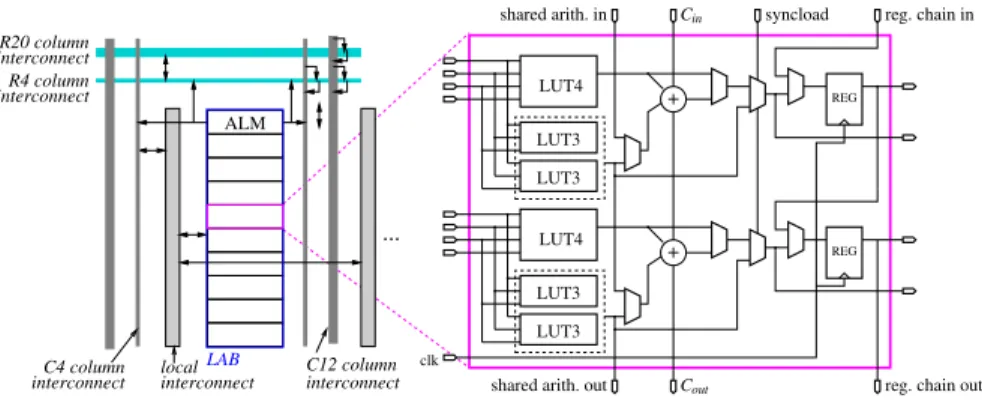
Figures 1 and 2 provide a schematic overview of the logic fabric of recent FPGAs from the two main FPGA vendors. The features of interest are the following.
CLB Cout SHIFTout Cin Cin SHIFTin Cout SLICEM2 SLICEM0 SLICEL1 SLICEL3 Matrix Switch VersaBlock General routing matrix Cin Cout clk direct 0 0 1 1 0 1 1 0 LUT4 LUT4 MUXFX REG REG MUXF5
Fig. 1 Schematic overview of the logic blocks in the Virtex 4. More recent devices are similar, with up to 6 inputs to the LUTs
+ + ... ALM R20 column R4 column interconnect interconnect interconnect C4 column local interconnect LAB interconnect C12 column Cin
shared arith. in syncload reg. chain in
reg. chain out Cout
shared arith. out
clk LUT3 LUT3 LUT4 LUT3 LUT3 LUT4 REG REG
2.1.1 Look-up tables
The logic fabric is based on look-up tables with α inputs and one output, with α = 4..6 for the FPGAs currently on the market, the most recent FPGAs having the largest α. These LUTs may be combined to form larger LUTs (for instance the MUXF5 multiplexer visible on Figure 1 serves this purpose). Conversely, they may be split into smaller LUTs, as is apparent on Figure 2, where two LUT3 may be combined into a LUT4, and two LUT4 into a LUT5.
As far as arithmetic is concerned, this LUT-based structure means that algorithms relying on the tabulation of 2αvalues have very efficient implementations in FPGAs.
Examples of such algorithms include multiplication or division by a constant (see Section 4.1) and function evaluation (see Section 6.2).
2.1.2 Fast carry propagation
The two families provide a fast connexion between neighbouring cells in a col-umn, dedicated to carry propagation. This connexion is fast in comparison to the general programmable routing which is slowed down by all the switches enabling this programmability. Compared to classical (VLSI oriented) hardware arithmetic, this considerably changes the rules of the game. For instance, most of the litera-ture regarding fast integer adders is irrelevant on FPGAs for additions smaller than 32 bits: the simple carry-ripple addition exploiting the fast-carry lines is faster, and consumes fewer resources, than the “fast adders” of the literature. Even for larger additions, the optimal solutions on FPGAs are not obtained by blindly applying the classical techniques, but by revisiting them with these new rules [64, 28, 58].
Fast carries are available on both Altera and Xilinx devices, but the detailed struc-ture differs. Both device families allow one to merge an addition with some compu-tations performed in the LUT. Altera devices are designed in such a way to enable the implementation of a 3-operand adder in one ALM level (see Figure 2).
2.1.3 DSP blocks
Embedded multipliers (18x18-bit signed) first appeared in Xilinx VirtexII devices in 2000, and were complemented by a DSP-oriented adder network in the Altera Stratix in 2003.
DSP blocks not only enhance the performance of DSP applications – and, as we will see, any application using multiplication–, they also make this performance more predictable.
Xilinx DSP blocks
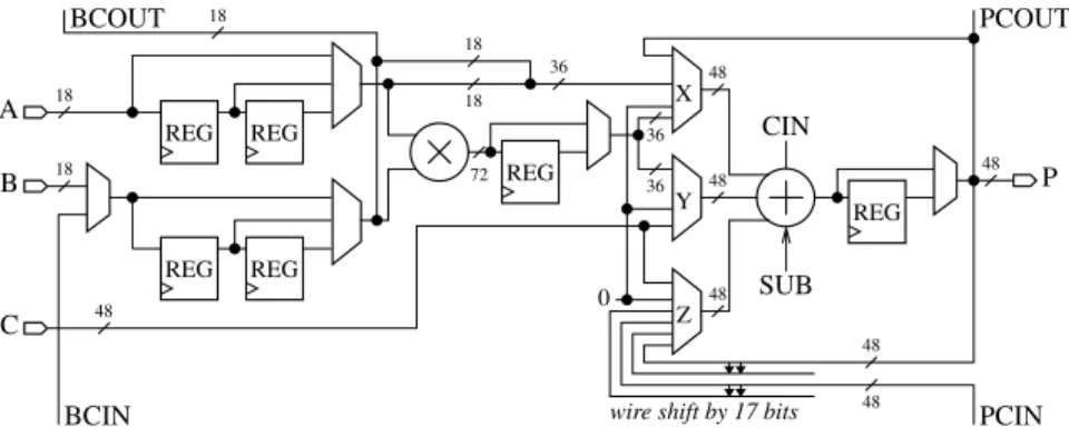
A simplified overview of the DSP48 block of Virtex-4 devices is depicted in Figure 3. It consists of one 18x18-bit two’s complement multiplier followed by a 48-bit sign-extended adder/subtracter or accumulator unit. The multiplier outputs two sub-products aligned on 36-bits. A 3-input adder unit can be used to add three external inputs, or the two sub-products and a third addend. The latter can be an accumulator (hence the feedback path) or an external input, coming either from global routing or from a neighboring DSP via a dedicated cascading line (PCIN). In this case this input may be shifted by 17 bits. This enables associating DSP blocks to compute large multiplications. In this case unsigned multiplications are needed, so the sign bit is not used, hence the value of 17.
These DSP blocks also feature internal registers (up to four levels) which can be used to pipeline them to high frequencies.
REG REG REG REG REG X Y Z 0 REG 18 18
wire shift by 17 bits
48 18 18 18 36 72 36 36 48 48 48 48 48 48 BCIN C B A BCOUT PCOUT P PCIN CIN SUB
Fig. 3 Simplified overview of the Xilinx DSP48
Virtex-5/-6/-7 feature similar DSP blocks (DSP48E), the main difference being a larger (18x25-bit, signed) multiplier. In addition the adder/accumulator unit can now perform several other operations such as logic operations or pattern detection. Virtex-6 and later add pre-multiplication adders within the DSP slice.
Altera DSP blocks
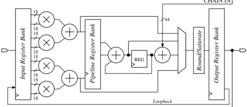
The Altera DSP blocks have a much larger granularity than the Xilinx ones. On StratixII-IV devices (Figure 4) the DSP block consists of four 18 x 18 bit (signed or unsigned) multipliers and an adder tree with several possible configurations, rep-resented on Figure 5. Stratix-III/-IV calls such DSPs half-DSPs, and pack two of them in a DSP block. In these devices, the limiting factor in terms of configurations (preventing us, for instance, to use them as 4 fully independent multipliers) is the number of I/Os to the DSP block. The variable precision DSP block in the StratixV devices is radically different: it is optimized for 27x27-bit or 18x36-bit, and a 36-bit
multiplier is implemented in two adjacent blocks. Additionally, all DSPs allow var-ious sum-of-two/four modes for increased versatility. Here also, neighbouring DSP blocks can be cascaded, internal registers allow high-frequency pipelining, and a loopback path enables accumulation. These cascading chains reduce resource con-sumption, but also latency: a sum-of-two 27-bit multipliers can be clocked at nomi-nal DSP speed in just 2 cycles.
When designing operators for these devices, it is useful to account for these dif-ferent features and try to fully exploit them. The full details can be found in the vendor documentation. REG Round/Satur ate 44 18 18 18 18 18 18 18 18 Pipeline Re gister Bank Loopback CHAIN IN CHAIN OUT Input Re gister Bank Output Re gister Bank
Fig. 4 Simplified overview of the StratixII DSP block, Stratix-III/-IV half-DSP block
38
72 55
37 37
Fig. 5 Main configurations of Stratix DSP. Leftmost can be used to compute a 36x36 bit product, rightmost to compute the product of complex numbers.
2.1.4 Embedded memories
Modern FPGAs also include small and fast on-chip embedded memories. In Xil-inx Virtex4 the embedded memory size is 18Kbits, and 36Kbits for Virtex5/6. The blocks support various configurations from 16K x 1-bit to 512 x 36-bit (1K for Vir-tex5/6).
Altera FPGAs offer blocks of different sizes. StratixII has 3 kinds of memory blocks: M512 (512-bit), M4K (4Kb) and M-RAM (512Kb); StratixIII-IV have a new family of memory blocks: MLAB (640b ROM/320b RAM), M9K (9Kbit, up
to 256x36-bit) and M144K (144Kbits, up to 2K x 72-bit); StratixV has MLAB and M20K (20Kbits, up to 512 x 40-bit).
In both families, these memories can be dual-ported, sometimes with restrictions.
2.2 Floating-point formats for reconfigurable computing
A floating-point (FP) number x is composed of a sign bit S, an exponent field E on wE bits, and a significand fraction F on wF bits. It is usually mandated that the
significand fraction has a 1 at its MSB: this ensures both uniqueness of representa-tion, and maximum accuracy in the case of a rounded result. Floating-point has been standardized in the IEEE-754 standard, updated in 2008 [40]. This standard defines common formats, the most usual being a 32-bit (the sign bit, 8 exponent bits, 23 significand bits) and a 64-bit format (1+12+53). It precisely specifies the basic op-erations, in particular the rounding behaviour. It also defines exceptional numbers: two signed infinities, two signed zeroes, subnormal numbers for a smooth underflow to zero, and NaN (Not a Number). These exceptional numbers are encoded in the extremal values of the exponent.
This standard was designed for processor implementations, and makes perfect sense there. However, for FPGAs, many things can be reconsidered. Firstly, a de-signer should not restrict himself to the 32-bit and 64-bit formats of IEEE-754: he should aim at optimizing both exponent and significand size for the application at hand. The floating-point operators should be fully parameterized to support this.
Secondly, the IEEE-754 encodings were designed to make the most out of a fixed number of bits. In particular, exceptional cases are encoded in the two extremal values of the exponent. However, managing these encodings has a cost in terms of performance and resource consumption [35]. In an FPGA, this encoding/decoding logic can be saved if the exceptional cases are encoded in two additional bits. This is the choice made by FloPoCo and other floating-point libraries. A small additional benefit is that this choice frees the two extremal exponent values, slightly extending the range of the numbers.
Finally, we choose not to support subnormal numbers support, with flushing to zero instead. This is the most controversial issue, as subnormals bring with them important properties such as (x − y = 0) ⇐⇒ (x = y), which is not true for FP numbers close to zero if subnormals are not supported. However the cost of sup-porting subnormals is quite high, as they require specific shifters and leading-one detectors [35]. Besides, one may argue that adding one bit of exponent brings in all the subnormal numbers, and more, at a fraction of the cost: subnormals are less relevant if the format is fully parameterized. We believe there hasn’t been a clear case for subnormal support in FPGA computing yet.
To sum up, Figure 6 depicts a FloPoCo number, whose value (always normalized) is
x= (−1)S× 1.F × 2E−E0 with E
E0is called the exponent bias. This representation of signed exponents (taken from
the IEEE-754 standard) is prefered over two’s complement, because it brings a use-ful property: positive floating-point numbers are ordered according to the lexico-graphic order of their binary representation (exponent and significand).
2 1 wE wF
E F
exn S
Fig. 6 The FloPoCo floating-point format.
3 Arithmetic efficiency and precision analysis
When implementing a given computation on an FPGA, the goal is usually to obtain an efficient design, be it to maximize performance, minimize the cost of the FPGA chip able to implement the computation, minimize the power consumption, etc. This quest for efficiency has many aspects (parallelism, operator sharing, pipeline balanc-ing, input/output throughputs, FIFO sizes, etc). Here, we focus on an often under-stated issue, which is fairly specific to numerical computation on FPGAs: arithmetic efficiency. A design is arithmetic-efficient if the size of each operator is as small as possible, considering the accuracy requirements of the application. Ideally, no bit should be flipped, no bit should be transfered that is not relevant to the final result.
Arithmetic efficiency is a relatively new concern, because it is less of an issue for classical programming: microprocessors offer a limited choice of registers and operators. The programmer must use 8-, 16-, or 64-bit integer arithmetic, or 32-or 64-bit floating-point. This is often very inefficient. F32-or instance, both standard floating-point formats are vastly overkill for most parts of most applications. In a processor, as soon as you are computing accurately enough, you are very probably computing much too accurately.
In an FPGA, there are more opportunities to compute just right, to the granularity of the bit. Arithmetic efficiency not only saves logic resources, it also saves routing resources. Finally, it also conserves power, all the more as there is typically more activity on the least significant bits.
Arithmetic efficiency is obtained by bit-width optimization, which in turn re-quires precision analysis. These issues have been the subject of much research, see for instance [57, 65, 47, 66] and references therein.
Range and precision analysis can be formulated as follows: given a computation (expressed as a piece of code or as an abstract circuit), label each of the interme-diate variables or signals with information about its range and its accuracy. The range is typically expressed as an interval, for instance variable V lies in the inter-val [−17, 42]. In a fixed-point context, we may deduce from the range of a signal the value of its most significand bit (MSB) which will prevent the occurence of any overflow. In a floating-point context, the range entails the maximum exponent that
the format must accomodate to avoid overflows. In both contexts, accurate determi-nation of the the ranges enables us to set these parameters just right.
To compute the range, some information must be provided about the range of the inputs – by default it may be defined by their fixed-point or floating-point for-mat. Then, there are two main methods for computing the ranges of all the signals: dynamic analysis, or static analysis.
Dynamic methods are based on simulations. They perform several runs using different inputs, chosen in a more or less clever way. The minimum and maximum values taken by a signal over these runs provides an attainable range. However, there is no guarantee in general that the variable will not take a value out of this range in a different run. These methods are in principle unsafe, although confidence can be attained by very large numbers of runs, but then these methods become very compute-intensive, especially if the input space is large.
Static analysis methods propagate the range information from the inputs through the computation, using variants of interval analysis (IA) [54]. IA provides range intervals that cover all the possible runs, and therefore is safe. However, it often overestimates these ranges, leading to bits at the MSB or exponent bits that will never be useful to actual computations. This ill-effect is essentially due to correla-tions between variables, and can be avoided by algebraic rewriting [27] (manual or automated), or higher-order variants of interval arithmetic such as affine arithmetic [47], polynomial arithmetic [12] or Taylor models. In case of loops, these methods must look for a fix point [66]. A general technique in this case is abstract interpre-tation [18].
Bit-width minimization techniques reduce the size of the data, hence reduce the size and power consumption of all the operators computing on these data. However, there are also less frequent, but more radical operator optimization opportunities. The remainder of this chapter reviews them.
4 Operator specialization
Operator specialization consists in optimizing the structure of an operator when the context provides some static (compile-time) property on its inputs that can be usefully exploited. This is best explained with some examples.
First, an operator with a constant operand can often be optimized somehow: • Even in software, it is well-known that cubing or extracting a square root is
sim-pler than using the pow function xy.
• For hardware or FPGAs, multiplication by a constant has been extensively stud-ied (although its complexity in the general case is still an open question). There exist several competing constant multiplication techniques, with different rele-vance domains: they are reviewed in Section 4.1.
• One of us has worked recently on the division by a small integer constant [25]. • However, on FPGA technology, there seems to be little to win on addition with a
It is also possible to specialize an operator thanks to more subtle relationships between its inputs. Here are two examples which will be expanded in 5.3:
• In terms of bit flipping, squaring is roughly twice cheaper than multiplying. • If two numbers have the same sign, their floating-point addition is cheaper to
implement than a standard addition: the cancellation case (which costs one large leading-zero counter and shifter) never happens [49].
Finally, many functions, even unary ones, can be optimized if their input is stati-cally known to lie within a certain range. Here are some examples.
• If a floating-point number is known to lie in [−π, π], its sine is much cheaper to evaluate than in the general case (no argument reduction) [21].
• If the range of the input to an elementary function is small enough, a low-degree polynomial approximation may suffice.
• etc.
Finally, an operator may have its accuracy degraded, as long as the demand of the application is matched. The most spectacular example is truncated multipliers: sacrificing the accuracy of the least significant bit saves almost half the area of a floating-point multiplier [67, 8]. Of course, in the FPGA context, the loss of preci-sion can be recovered by adding one bit to the mantissa, which has a much lower cost.
The remainder of this section focuses on specializations of the multiplication, but designers on FPGAs should keep in mind this opportunity for many other oper-ations.
4.1 Multiplication and division by a constant
Multiplication by constants has received much attention in the literature, especially as many digital signal processing algorithms can be expressed as products by con-stant matrices [62, 52, 13, 72]. There are two main families of algorithms. Shift-and-add algorithms start from the construction of a standard multiplier and simplify it, while LUT-based algorithm tabulate sub-products in LUTs and are thus more specific to FPGAs.
4.1.1 Shift and add algorithms
Let C be a positive integer constant, written in binary on k bits:
C=
k
∑
i=0
ci2i with ci∈ {0, 1}.
Let X a p-bit integer. The product is written CX = ∑ki=02iciX, and by only
In the following, we will note this using the shift operator<<, which has higher priority than + and −. For instance 17X = X + X<<4.
If we allow the digits of the constant to be negative (ci∈ {−1, 0, 1}) we obtain a
redundant representation, for instance 15 = 01111 = 10001 (16 − 1 written in signed binary). Among the representations of a given constant C, we may pick up one that minimises the number of non-zero bits, hence of additions/subtractions. The well-known canonical signed digits recoding (or CSD, also called Booth recoding [36]) guarantees that at most k/2 bits are non-zero, and in average k/3.
The CSD recoding of a constant may be directly translated into an architecture with one addition per non-zero bit, for instance 221X = 1001001012X= X<<8 +
(−X<<5 + (−X<<2 + X )). With this right-to-left parenthesing, all the additions are actually of the same size (the size of X ): in an addition X<<s + P, the s lower bits of the result are those of P and do not need to participate to the addition.
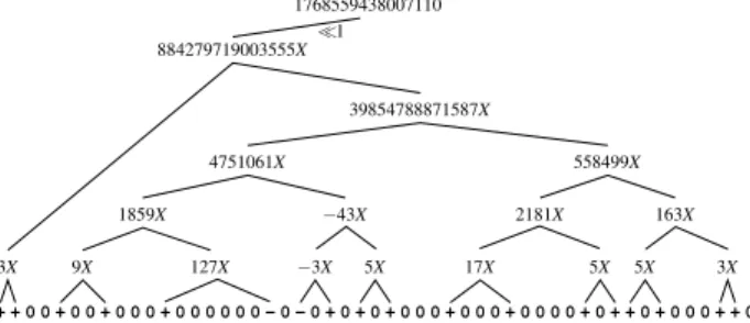
For large constants, a binary tree adder structure can be constructed out of the CSD recoding of the constant as follows: non-zero bits are first grouped by 2, then by 4, etc. For instance, 221X = (X<<8 − X<<5) + (−X<<2 + X ). Shifts may also be reparenthesised: 221X = (X<<3 − X )<<5 + (−X<<2 + X ). After doing this, the leaves of the tree are now multiplications by small constants: 3X , 5X , 7X , 9X ... Such a smaller multiple will appear many times in a larger constant, but it may be computed only once: thus the tree is now a DAG (direct acyclic graph), and the number of additions is reduced. A larger example is shown on Figure 7. This new parenthesing reduces the critical path: for k non-zero bits, it is now of dlog2ke additions instead of k in the previous linear architecture. However, additions in this DAG are larger and larger.
This simple DAG construction is the current choice in FloPoCo, but finding the optimal DAG is still an open problem. There is a wide body of literature on con-stant multiplication, minimizing the number of additions [9, 19, 37, 72, 69], and, for hardware, also minimizing the total size of these adders (hence the logic consump-tion in an FPGA) [19, 37, 1, 38]. It has been shown that the number of adders in constant multiplication problem is sub-linear in the number of non-zero bits [23]. Exhaustive exploration techniques [19, 37, 69] lead to less than 4 additions for any constant of size smaller than 12 bits, and less than 5 additions for sizes smaller
0 0 0 0 0 0 0 0 0 0 + 0 + 0 + 0 + 0 0 0 0 0 0 0 0 0 0 0 0 + + 0 0 + 0 + − 0 − + + 0 + 0 + + 0 + + + 0 5X 5X 17X 5X −3X 3X 9X 127X 3X 39854788871587X 884279719003555X 558499X 4751061X −43X 1859X 2181X 163X 1768559438007110 <<1
Fig. 7 Binary DAG architecture for a multiplication by 1768559438007110 (the 50 first bits of the mantissa of π).
than 19 bits. They become impractical beyond these sizes, and heuristics have to be used. Lef`evre’s algorithm [48] looks for maximal repeating bit patterns (in direct or complemented form) in the CSD representation of the constant, then proceeds recursively on these patterns. Experimentally, the number of additions, on randomly generated constants of k bits, grows as O(k0.85). However, this algorithm does not
currently try to minimize the total size of the adders [14], contrary to Gustafsson et al [37].
All the previous dealt with multiplication by an integer constant. Multiplying by a real constant (in a fixed-point or floating-point context) raises the additional issue of first approximating this constant by a fixed-point number. Gustafsson and Qureshi suggested to represent a real constant on more than the required number of bits, if it leads to a shift-and-add architecture with fewer additions [38]. This idea was exploited analytically for rational constants, which have a periodic binary representation [24].
4.1.2 Table-based techniques
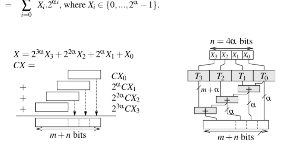
On most FPGAs, the basic logic element is the look-up-table, a small memory ad-dressed by α bits. The KCM algorithm (which probably means “constant (K) Co-efficient Multiplier”), due to Chapman [15] and further studied by Wirthlin [76] is an efficient way to use these LUTs to implement a multiplication by an integer constant.
This algorithm, described on Figure 8, consists in breaking down the binary decomposition of an n-bit integer X into chunks of α bits. This is written as
X = dn αe−1
∑
i=0 Xi.2α i, where Xi∈ {0, ..., 2α− 1}. + + + CX= CX0 22αCX2 2αCX 1 23αCX3 T3 T2 T1 T0+
+
+
α α α m+ n bits m+ n bits n= 4α bits X0 X1 X3 X2 X= 23αX3+ 22αX2+ 2αX1+ X0 m+ αFig. 8 The KCM LUT-based method (integer × integer)
The product of X by an m-bit integer constant C becomes CX = ∑d n αe
i=0CXi.2−αi.
KCM trick is to read these CXifrom a table of pre-computed values Ti, indexed by
Xi, before summing them.
The cost of each table is one FPGA LUT per output bit. The lowest-area way of computing the sum is to use a rake of dn
αe in sequence, as shown on Figure 8: here
again, each adder is of size m + α, because the lower bits of a product CXican be
output directly. If the constant is large, an adder tree will have a shorter latency at a slightly larger area cost. The area is always very predictible and, contrary to the shift-and-add methods, almost independent on the value of the constant (still, some optimizations in the tables will be found by logic optimizers).
There are many possible variations on the KCM idea.
• As all the tables contain the same data, a sequential version can be designed. • This algorithm is easy to adapt to signed numbers in two’s complement. • Wirthlin [76] showed that if we split the input in chunks of α − 1 bits, then one
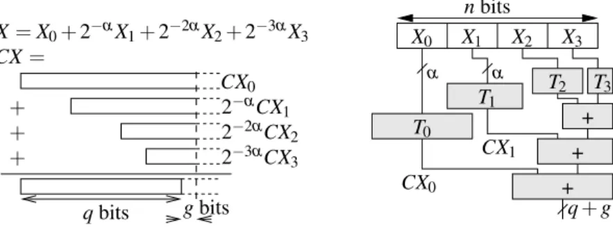
row of LUT can integrate both the table and the corresponding adder, and still exploit the fast-carry logic of Xilinx circuits: this reduces the overall area. Altera FPGAs don’t need this trick thanks to their embedded full adder (see Figure 2). • It can be adapted to fixed-point input and, more interesting, to an arbitrary real
constant C, for instance log(2) in [30] or FFT twiddle factors in [33]. Figure 9 describes this case. Without loss of generality, we assume a fixed-point input in [0, 1): it is now written on n bits as X = ∑d
n αe−1
i=0 Xi.2−αi where Xi ∈
{0, ..., 2α− 1}. Each product CX
i now has an infinite number of bits. Assume
we want an q-bit result with q ≥ n. We tabulate in LUTs each product 2iαCX i
on just the required precision, so that its LSB has value 2−guwhere u is the ulp of the result, and g is a number of guard bits. Each table may hold the correctly rounded value of the product of Eiby the real value of C to this precision, so
en-tails an error of 2−g−1ulp. In the first table, we actually store CX0+ u/2, so that
the truncation of the sum will correspond to a rounding of the product. Finally, the value of g is chosen to ensure 1-ulp accuracy.
CX0 CX1 + + + CX= 2−3αCX3 2−αCX1 2−2αCX2 CX0 + + + T3 T2 X0 X1 X2 X3 T1 α T0 α nbits X= X0+ 2−αX1+ 2−2αX2+ 2−3αX3 q+ g qbits gbits
4.1.3 Other variations of single-constant multiplication
Most algorithms can be extended to a floating-point version. As the point of the constant doesn’t float, the main question is whether normalization and rounding can be simpler than in a generic multiplication [14].
For simple rational constants such as 1/3 or 7/5, the periodicity of their binary representations leads to optimizations both in KCM and shift-and-add methods [24]. The special case corresponding to the division by a small integer constant is quite useful: Integer division by 3 (with remainder) is used in the exponent processing for cube root, and division by 5 is useful for binary to decimal conversion. Fixed-point division by 3 (actually 6 or 24, but the power of two doesn’t add to the complexity) enables efficient implementations of sine and cosine based on parallel evaluation of their Taylor series. Floating-point division by 3 is used in the Jacobi stencil algo-rithm. In addition to techniques considering division by a constant as the multipli-cation by the inverse [24], a specific LUT-based method can be derived from the division algorithm [25].
4.1.4 Multiple constant multiplication
Some signal-processing transforms, in particular finite impulse response (FIR) fil-ters, need a given signal needs to be multiplied by several constants. This allows further optimizations: it is now possible to share sub-constants (such as the in-termediate nodes of Figure 7) between several constant multipliers. Many heuris-tics have been proposed for this Multiple Constant Multiplication (MCM) problem [62, 13, 52, 72, 1].
A technique called Distributed Arithmetic, which predates FPGA [74] , can be considered a generalization of the KCM technique to the MCM problem.
4.1.5 Choosing the best approach in a given context
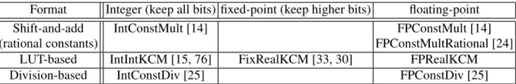
To sum up, there is plenty of choice in terms of constant multiplication or division in an FPGA. Table 2 describes the techniques implemented in the FloPoCo tool at the time of writing. This is work in progress.
As a rule of thumb, for small inputs, KCM should be preferred, and for simple constants, shift-and-add should be preferred. In some cases the choice is obvious: for instance, to evaluate a floating-point exponential, we have to multiply an exponent (a small integer) by log(2), and we need many more bits on the result: this is a case for KCM, as we would need to consider many bits of the constant. In most usual cases, however, the final choice should probably be done on a trial and error basis.
Format Integer (keep all bits) fixed-point (keep higher bits) floating-point
Shift-and-add IntConstMult [14] FPConstMult [14]
(rational constants) FPConstMultRational [24]
LUT-based IntIntKCM [15, 76] FixRealKCM [33, 30] FPRealKCM
Division-based IntConstDiv [25] FPConstDiv [25]
Table 2 Constant multiplication and division algorithms in FloPoCo 2.3.1
4.2 Squaring
If one computes, using the pen-and-paper algorithm learnt at school, the square of a large number, one will observe that each of the digit-by-digit products is computed twice. This holds also in binary: formally, we have
X2= ( n−1
∑
i=0 2ixi)2= n−1∑
i=0 22ixi +∑
0<i< j<n 2i+ j+1xixjand we have a sum of roughly n2/2 partial products, versus n2for a standard n-bit multiplication. This is directly useful if the squarer is implemented as LUTs. In addition, a similar property holds for a splitting of the input into several subwords:
(2kX1+ X0)2= 22kX12+ 2 · 2kX1X0+ X02 (1) (22kX2+ 2kX1+ X0)2= 24kX22+ 22kX12+ X02 + 2 · 23kX 2X1 + 2 · 22kX2X0 + 2kX 1X0 (2)
Computing each square or product of the above equation in a DSP block, yields a reduction of the DSP count from 4 to 3, or from 9 to 6. Besides, this time, it comes at no arithmetic overhead. Some of the additions can be computed in the DSP blocks, too. This has been studied in details in [29].
Squaring is a specific case of powering, i.e. computing xpfor a constant p.
Ad-hoc, truncated powering units have been used for function evaluation [20]. These are based on LUTs, and should be reevaluated in the context of DSP blocks.
5 Operator fusion
Operator fusion consists in building an atomic operator for a non-trivial mathe-matical expression, or a set of such expressions. The recipe is here to consider the mathematical expression as a whole and to optimize each operator in the context of the whole expression. The opportunities for operator fusion are unlimited, and the purpose of this section is simply to provide a few examples which are useful enough to be provided in an operator generator such as FloPoCo.
5.1 Floating-point sum-and-difference
In many situations, the most pervasive of which is probably the Fast Fourier Trans-form (FFT), one needs to compute the sum and the difference of the same two values. In floating-point, addition or subtraction consists in the following steps [56]: • alignment of the significands using a shifter, the shift distance being the exponent
difference;
• effective sum or difference (in fixed-point);
• in case of effective subtraction leading to a cancellation, leading zero count (LZC) and normalization shift, using a second shifter;
• final normalization and rounding.
We may observe that several redundancies exist if we compute in parallel the sum and the difference of the same values:
• The exponent difference and alignment logic is shared by the two operations. • The cancellation case will appear at most once, since only one of the operations
will be an effective subtraction, so only one LZC and one normalization shifter is needed.
Summing up, the additional cost of the second operation, with respect to a clas-sical floating-point adder, is only its effective addition/subtraction, and its final nor-malization and rounding logic. Numerically, a combined sum-and-difference opera-tor needs about one third more logic than a standard adder, and has the same latency.
5.2 Block floating-point
Looking back at the FFT, it is essentially based on multiplication by constants, and the previous sum-and-difference operations. In a floating-point FFT, operator fusion can be pushed a bit further, using a technique called block floating-point [41], first used in the 1950s, when floating point arithmetic was implemented in software, and more recently applied to FPGAs [3, 5]. It consists in an initial alignment of all the input significands to the largest one, which brings them all to the same exponent (hence the phrase “block floating point”). After this alignment, all the computations (multiplications by constants and accumulation) can be performed in fixed point, with a single normalization at the end. Another option, if the architecture imple-ments only one FFT stage and the FFT loops on it, is to perform the normalization of all the values to the largest (in magnitude) of the stage.
Compared with the same computation using standard floating-point operators, this approach saves all the shifts and most of the normalization logic in the inter-mediate results. The argument is that the information lost in the initial shifts would have been lost in later shifts anyway. However, a typical block floating-point im-plementation will accumulate the dot product in a fixed-point format slightly larger
than the input significands, thus ensuring a better accuracy than that achieved using standard operators.
Block floating-point techniques can be applied to many signal processing trans-forms involving the product of a signal vector by a constant vector. As it eventually converts the problem to a fixed-point one, the techniques for multiple constant mul-tiplication listed in 4.1.4 can be used.
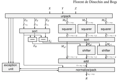
5.3 Floating-point sum of squares
We conclude this section with the example of a large fused operator that combines several of the FPGA-specific optimizations discussed so far. The datapath described on Figure 10 inputs three point numbers X , Y and Z, and outputs a floating-point value for X2+ Y2+ Z2. Compared to a more naive datapath built out of
stan-dard adders and multiplier, it implements several optimizations:
• It uses squarers instead of multipliers, as suggested in 4.2. These can even be truncated squarers.
• As squares are positive, it can dispose of the leading-zero counters and shifters that, in standard floating-point additions, manage the possible cancellation in case of subtraction [49].
• It saves all the intermediate normalizations and rounding.
• It computes the three squares in parallel and feeds them to a three-operand adder (which is no more expensive than a two-operand adder in Altera devices) instead of computing the two additions in sequence.
• It extends the fixed-point datapath width by g = 3 guard bits that ensure that the result is always last-bit accurate, where a combination of standard operators would lead to up to 2.5 ulps of error. This is the value of g for a sum of three squares, but it can be matched to any number of squares to add, as long as this number is known statically.
• It reflects the symmetry of the mathematical expression X2+ Y2+ Z2, contrary
to a composition of floating-point operators which computes (X2+ Y2) + Z2,
leading to slightly different results if X and Z are permuted.
Compared to a naive assembly of three point multipliers and two floating-point adders, the specific architecture of Figure 10 thus significantly reduces logic count, DSP block count and latency, while being more accurate than the naive data-path. For instance, for double-precision inputs and outputs on Virtex-4, slice count is reduced to 4480 to 1845, DSP count is reduced from 27 to 18, and latency is re-duced from 46 to 16 cycles, for a frequency of 362 MHz (post-synthesis) which is nominal on this FPGA.
1 + wF 1 + wF 1 + wF 2 + wF+ g 2 + wF+ g 2 + wF+ g 2 + wF+ g 2 + wF+ g 2 + wF+ g EC EB MB2 MC2 X Y Z MX EZ EY EX MY MZ R 4 + wF+ g MA2 wE wE wE wE+ wF shifter sort sort squarer squarer
shifter squarer unit exception add normalize/pack unpack
Fig. 10 A floating-point sum-of-squares (for wEbits of exponent and wFbits of significand)
5.4 Towards compiler-level operator fusion
Langhammer proposed an optimizing floating-point datapath compiler [46] that: • detects clusters of similar operations and uses a fused operator for the entire
cluster;
• detects dependent operations and fuses the operators by removing or simplifying the normalization, rounding steps and alignment steps of the next operation. To ensure high accuracy in spite of these simplifications, the compiler relies on additional accuracy provided for free by the DSP blocks. The special floating-point formats used target accuracy “soft spots” for recent Altera DSP blocks (StratixII-IV) which is 36 bits. For instance, in single-precision (24 mantissa bits) the adders use an extended, non-normalized mantissa of up to 31 bits which, when followed by a multiplier stage uses the 36-bit multiplier mode on the 31-bit operands. For this stage as well, an extended mantissa allows for late normalizations while preserving accuracy. The optimizations proposed by Langhammer are available in Altera’s DSP Builder Advanced tool [60].
6 Exotic operators
This section presents in details three examples of operators that are not present in processors, which gives a performance advantage to FPGAs. There are many more examples, from elementary functions to operators for cryptography.
6.1 Accumulation
Summing many independent terms is a very common operation: scalar products, matrix-vector and matrix-matrix products are defined as sums of products, as are most digital filters. Numerical integration usually consists in adding many elemen-tary contributions. Monte-Carlo simulations also involve sums of many independent terms.
Depending on the fixed/floating-point arithmetic used and the operand count there are several optimization opportunities.
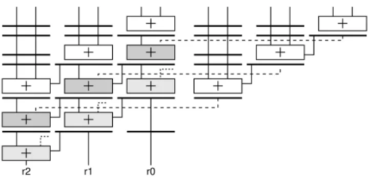
When having to sum a fixed, relatively small number of terms arriving in paral-lel, one may use adder trees. Fixed-point adder trees benefit from adder support in the FPGA fabric (ternary adder trees can be built on Altera FPGAs). If the preci-sion is large, adders can be pipelined [28] and tessellated [60] for reducing latency and resources (Figure 11). Floating-point adder trees for positive data may use a dedicated fused operator similar to the one in Figure 10 for the sum-of-squares. Otherwise, one may rely on the techniques presented by Langhammer for datap-ath fusion which, depending on the operator count combine clustering and delayed normalizations [46].
r2 r1 r0
Fig. 11 Fixed-point accumulation for small operand count based on a tessellated adder tree
For an arbitrary number of summands arriving sequentially, one needs an accu-mulator, conceptually described by Figure 12. A fixed-point accumulators may be built out of a binary adder with a feedback loop. This allows good performances for moderate-size formats: as a rule of thumb, a 32-bit accumulator can run at the FPGA nominal frequency (note also that a larger hard accumulator is available is modern DSP blocks). If the addition is too wide for the ripple-carry propagation to take place in one clock cycle, a redundant carry-save representation can be used for the accumulator. In FPGAs, thanks to fast carry circuitry, a high-radix carry save (HRCS), breaking the carry propagation typically every 32 bits, has a very low area overhead.
Building an efficient accumulator around a floating-point adder is more involved. The problem is that FP adders have long latencies: typically l = 3 cycles in a
proces-accumulated value register input (summand)
Fig. 12 An accumulator
sor, up to tens of cycles in an FPGA. This long latency means that an accumulator based on an FP adder will either add one number every l cycles, or compute l in-dependent sub-sums which then have to be added together somehow. One special case are large matrix operations [78, 10], when l parallel accumulations can be in-terleaved. Many programs can be restructured to expose such sub-sum parallelism [2].
In the general case, using a classical floating point adder of latency l as the adder of Figure 12, one is left with l independent sub-sums. The log-sum technique adds them using dlog2le adders and intermediate registers [68, 39]. Sun and Zambreno suggest that l can be reduced by having two parallel accumulator memories, one for positive addends and one for negative addends: this way, the cancellation detection and shift can be avoided in the initial floating-point accumulator. This, however, becomes inaccurate for large accumulations whose result is small [68].
Additionally, an accumulator built around a floating-point adder is inefficient, because the significand of the accumulator has to be shifted, sometimes twice (first to align both operands and then to normalise the result). These shifts are in the critical path of the loop. Luo and Martonosi suggested to perform the alignment in two steps, the finest part outside of the loop, and only a coarse alignment inside [50]. Bachir and David have investigated several other strategies to build a single-cycle accumulator, with pipelined shift logic before, and pipelined normalization logic after [7]. This approach was suggested in earlier work by Kulisch, targetting microprocessor floating-point units. Kulisch advocated the concept of an exact ac-cumulator as “the fifth floating-point operation”. Such an acac-cumulator is based on a very wide internal register, covering the full floating-point range [43, 44], and ac-cessed using a two-step alignment. One problem with this approach is that in some situations (long carry propagation), the accumulator requires several cycles. This means that the incoming data must be stalled, requiring more complex control. This is also the case in [50].
For FPGA-accelerated HPC, one critics to all previous approaches to universal accumulators is that they are generally overkill: they don’t compute just-right for the application. Let us now consider how to build an accumulator of floating-point numbers which is tailored to the numerics of an application. Specifically, we want to ensure that it never overflows and that it eventually provides a result that is as accurate as the application requires. Moreover, it is also designed around a single-cycle accumulator. We present this one [32] in detail as it exhibits many of the techniques used in previously mentioned works.
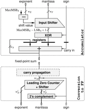
The accumulator holds the accumulation result in fixed-point format which al-lows removing any any alignments from the loop’s critical path. It is depicted in Figure 13. Single-cycle accumulation at arbitrary frequency is ensured by using an HRCS accumulator if needed.
The bottom part of Figure 13 presents a component which converts the fixed point accumulator back to floating-point. It makes sense to consider this as a sepa-rate component, beause this conversion may be performed in software if the running value of the accumulation is not needed (e.g. in numerical integration applications). In other situations (e.g. matrix-vector product), several accumulators can be sched-uled to share a common post-normalization unit. In this unit, the carry-propagation box converts the result into non-redundant format in the case when HCRS is used.
Accumulator Conversion to FP wA shift value mantissa carry in MaxMSBX− LSBA+ 1 MaxMSBX exponent wE wF sign mantissa sign exponent fixed-point sum registers w0 F wA w0 E
Leading Zero Counter + Shifter carry propagation
Input Shifter
2’s complement XOR
Fig. 13 The proposed accumulator (top) and post-normalisation unit (bottom).
The parameters of the accumulator are explained with the help of Figure 14: • MSBAis the position of the most-significant bit (MSB) of the accumulator. If the
maximal expected running sum is smaller than 2MSBA, no overflow ever occurs. • LSBAis the position of the least-significant bit of the accumulator and determines
the final accumulation accuracy.
• MaxMSBX is the maximum expected position of the MSB of a summand.
summand is much smaller in magnitude than the final sum. In this case, providing MaxMSBX< MSBAwill save hardware in the input shifter.
0 0 0 0 0 0 0 0 0 0 0 0 0 0 0 0 0 0 0 0 0 0 0 0 0 0 0 0 0 0 0 0 0 0 0 0 1 1 1 1 0 0 0 1 1 1 1 1 1 1 1 1 1 1 1 1 1 1 1 1 0 0 1 1 1 0 0 1 1 1 0 1 1 0 1 0 0 0 0 1 1 1 1 1 wA = MSBA− LSBA+ 1 Accumulator wF+ 1 LSBA= −12 MaxMSBX= 8 MSBA= 16 fixed point Summands (shifted mantissas)
Fig. 14 Accumulation of floating-point numbers into a large fixed-point accumulator
This parameters must be set up in an application-dependent way by considering the numerics of the application to be solved. In many cases, this is easy, because gross overestimation have a moderate impact: taking a margin of three orders of magnitude on MSBA, for instance, adds only ten bits to the accumulator size [32].
6.2 Generic polynomial approximation
Polynomial approximation is a invaluable tool for implementing fixed-point func-tions (which are also the basis of many floating-point ones) in hardware. Given a function f (x) and an input domain, polynomial approximation starts by finding a polynomial P(x) which approximates f (x). There are several methods for obtaining these polynomials including: the Taylor and Chebyshev series, or the Remez algo-rithm, a numerical routine that under certain conditions converges to the Minimax polynomial (the polynomial which minimizes the maximum error between f and P).
There is a strong dependency between the size of the input interval, the polyno-mial degree and the approximation accuracy: a higher degree polynopolyno-mial increases accuracy but also degrades implementation performance or cost. Piecewise poly-nomial approximation splits the input range into subintervals and uses a different polynomial pifor each subinterval. This scalable range reduction technique allows
reaching an arbitrary accuracy for fixed polynomial degree d. A uniform segmenta-tion scheme, where all subintervals have the same size, has the advantage that inter-val decoding the is straightforward, just using he leading bits of x. Non-uniform range reduction schemes like the power-of-two segmentation [16] have slightly
more complex decoding requirements but can enable more efficient implementation of some functions.
Given a polynomial, there are many possible ways to evaluate it. The HOTBM method [20] uses the developed form p(y) = a0+ a1y+ a2y2+ ... + adyd and
at-tempts to tabulate as much of the computation as possible. This leads to a short-latency architecture since each of the aiyimay be evaluated in parallel and added
thanks to an adder tree, but at a high hardware cost. Conversly, the Horner eval-uation scheme minimizes the number of operations, at the expense of latency: p(y) = a0+ y × (a1+ y × (a2+ .... + y × ad)...) [26]. Between these two extremes,
intermediate schemes can be explored. For large degrees, the polynomial may be decomposed into an odd and an even part: p(y) = pe(y2) + y × po(y2). The two
sub-polynomial may be evaluated in parallel, so this scheme has a shorter latency than Horner, at the expense of the precomputation of x2and a slightly degraded accuracy. Many variations on this idea, e.g. the Estrin scheme, exist [55]. A polynomial may also be refactored to trade multiplications for more additions [42], but this idea is mostly incompatible with range reduction.
When implementing an approximation of f in hardware, there are several error sources which, summed-up (εtotal) determine the final implementation accuracy. For
arithmetic efficiency, we aim at faithful rounding, which means that εtotalmust be
smaller than the weight of the LSB of the result, noted u. This error is decomposed as follows: εtotal= εapprox+ εeval+ εfinalroundwhere:
• εapproxis the approximation error, the maximum absolute difference between any
of the polynomials piand the function over its interval. The open-source Sollya
tool [17] offers the state of the art for both polynomial approximation and a safe computation of εapprox.
• εevalis the total of all rounding and truncation errors committed during the
eval-uation. These can be made arbitrarily small by adding g guard bits to the LSB of the datapath.
• εfinalroundis the error corresponding rounding off the guard bits from the evaluated
polynomial to obtain a result in the target format. It is bounded by u/2.
Given that εfinalround has a fixed bound (u/2), the aim is to balance the
approx-imation and evaluation error such that the final error remains smaller than u. One idea is to look for polynomials such that εapprox< u/4. Then, the remaining error
budget allocated to the evaluation error: εeval< u/2 − εapprox.
FloPoCo implements this process (more details in [26]), and builds the archi-tecture depicted in Figure 15. The datapath is optimized to compute just right at each point, truncating all the intermediate results to the bare minimum and using truncated multipliers [75, 8].
101 10 0 0 1 0 1 0 1001 . polynomial index a1 P2k−1 P1 P0 y ˜ y1 y˜d ad a0 Coefficient ROM x round r
Fig. 15 Function evaluation using piecewise polynomial approximation and a Horner datapath computing just right
6.3 Putting it all together: a floating-point exponential
We conclude this section by presenting, on Figure 16 a large operator that combines many of the techniques reviewed so far:
• a fixed-point datapath, surrounded by shifts and normalizations, • constant multiplications by log(2) and 1/log(2),
• tabulation of pre-computed values in the eAbox,
• polynomial approximation for the eZ− Z − 1 box,
• truncated multipliers, and in general computing just right everywhere. The full details can be found in [30].
Roughly speaking, this operator consumes an amount of resource comparable to a floating-point adder and a floating-point multiplier together. It may be fully pipelined to the nominal frequency of an FPGA, and its throughput, in terms of exponentials computed per second, is about ten times the throughput of the best (software) implementations in microprocessors. In comparison, the throughput of floating points adders and multipliers is ten times less than the corresponding (hard-ware) processor implementation. This illustrates the potential of exotic operators in FPGAs.
7 Operator performance tuning
Designing an arithmetic operator involves many trade-offs, most often between per-formance and resource consumption. The architectures of functionnaly identical op-erators in microprocessors targetting different markets can can widely differ: com-pare for instance two functionally identical, standard fused multiply-and-add (FMA)
more accurately than needed! Never compute polynomial Constant multipliers precomputed ROM generic multiplier truncated evaluator Shift to fixed−point normalize / round Fixed-point X SX EX FX A Z E E ×1/ log(2) × log(2) eA eZ− Z − 1 Y R 1 + wF + g wF + g − k wF + g + 2 − k MSB wF + g + 2 − k wF + g + 1 − k MSB wF + g + 1 − 2k 1 + wF + g wE + wF + g + 1 wE + 1 wE + wF + g + 1 wE + wF + g + 1 k
Fig. 16 Architecture of a floating-point exponential operator.
operators published in the same conference, one for high-end processors [11], the other for embedded processors [51]. However, for a given processor, the architecture is fixed and the programmer has to live with it.
In FPGAs, we again have more freedom: A given operator can be tuned to the performance needs of a given application. This applies to all the FPGA-specific op-erators we surveyed, but also to classical, standard opop-erators such as plain addition and subtraction.
Let us review a few aspects of this variability which an FPGA operator library or generator must address.
7.1 Algorithmic choices
The most fundamental choice is the choice of the algorithm used. For the same function, widely different algorithms may be used. Here are but a few examples.
• For many algebraic or elementary functions, there is a choice between multiplier-based approaches such as polynomial approximation [61, 20, 70, 16, 26] or Newton-Raphson iterations [55, 73, 45], and digit-recurrence techniques, based essentially on table look-ups and additions, such as CORDIC and its derivatives for exponential, logarithm, and trigonometric functions [71, 4, 55, 77, 63], or the SRT family of algorithms for division and square root [36]). Polynomials have lower latency but consume DSP blocks, while digit-recurrence consume only logic but have a larger latency. The best choice here depends on the format, on the required performance (latency and frequency), on the capabilities of the tar-get FPGA, and also on the global allocation of resources within the application (are DSP a scarce resource or not?).
• Many algorithms replace expensive parts of the computations with tables of pre-computed values. With their huge internal memory bandwidth, FPGAs are good candidates for this. For instance, multiplication modulo some constant (a basic operator for RNS arithmetic or some cryptography applications) can be com-puted out of the formula X × Y mod n = ((X + Y )2− (X − Y )2)/4 mod n,
where the squares modulo n can be tabulated (this is a 1-input table, whereas tab-ulating directly the product modulo n would require a 2-input table of quadrat-ically larger size). Precomputed values are systematquadrat-ically used for elementary functions, for instance the previous exponential, for single-precision, can be built out of one 18-Kbits dual-port memory (holding both boxes eAand eZ− Z − 1 of
Figure 16) and one 18x18 multiplier [30]. They are also the essence of the mul-tipartite [34] and HOTBM [20] generic function approximation methods. Such methods typically offer a trade-off between computation logic, table size, and performance. Their implementation should expose this trade-off, because the op-timal choice will often be application-dependent.
• In several operators, such as addition or logarithm, the normalization of the result requires a leading-zero counter. This can be replaced with a leading-zero antic-ipator (LZA) which runs in parallel of the significand datapath, thus reducing latency [56].
• In floating-point addition, besides the previous LZA, several algorithmic tricks reduce the latency at the expense of area. A dual-path adder implements a sep-arate datapath dedicated to cancellation cases, thus reducing the critical path of the main datapath.
• The Karatsuba technique can be used to reduce DSP consumption of large mul-tiplications at the expense of more additions [29].
7.2 Sequential versus parallel implementation
Many arithmetic algorithms are sequential in nature: they can be implemented either as a sequential operator requiring n cycles on hardware of size n with a throughput of one result every n cycle , or alternatively as a pipelined operator requiring n
cycles on hardware of size n × s with a throughput of one result per cycle. Classical examples are SRT division or square root [36] and CORDIC [4].
Multiplication belongs to this class, too, but with the advent of DSP blocks the granularity has increased. For instance, using DSP blocks with 17x17-bit multipli-ers, a multiplication of 68x68 (where 68 = 4 × 17) can be implemented as either a sequential process consuming 4 DSP blocks with a throughput of one result every 4 cycles, or as a fully pipelined operator with a throughput of 1 result per cycle, but consuming 16 DSP blocks.
7.3 Pipelining tuning
Finally, any combinatorial operator may be pipelined to an arbitrary depth, exposing a trade-off between frequency, latency, and area. FPGAs offer plenty of registers for this: there is one register bit after each LUT, and many others within DSP blocks and embedded memories. Using these is in principle for free: going from a com-binatorial to a deeply pipelined implementation essentially means using otherwise unused resources. However, a deeper pipeline will need more registers for data syn-chronization, and put more pressure on routing.
FloPoCo inputs a target frequency, and attempts to pipeline its operators for this frequency [31]. Such frequency-directed pipelining is, in principle, compositional: one can build a large pipeline operating at frequency f out of sub-components op-erating themselves at frequency f .
8 Open issues and challenges
We have reviewed many opportunities of FPGA-specific arithmetic, and there are are many more waiting to be discovered. We believe that exploiting these opportu-nities is a key ingredient of successful HPC on FPGA. The main challenges is now probably to put this diversity in the hands of programmers, so that they can exploit it in a productive way, without having to become arithmetic experts themselves. This section explores this issue, and is concluded with a review of possible FPGA enhancements that would improve their arithmetic support.
8.1 Operator specialization and fusion in high-level synthesis flows
In the HLS context, many classical optimizations performed by usual standard com-pilers should be systematically generalized to take into account opportunities of operator specialization and fusion. Let us take just one example. State-of-the-art compilers will consider replacing A + A by 2A, because this is an optimization that
is worth investigating in software: the compiler balances using one instruction, or another. HLS tools are expected to inherit this optimization. Now consider replacing A∗ A by A2: this is syntactically similar, and it also consists in replacing one
oper-ator with another. But it is interesting only on FPGAs, where squaring is cheaper. Therefore, it is an optimization that we have to add to HLS tools.
Conversely, we didn’t dare describe doubling as a specialization of addition, or A− A = 0 as a specialization of subtraction: it would have seemed too obvious. However they are, and they illustrate that operator specialization should be con-sidered one aspect of compiler optimization, and injected in classical optimization problems such as constant propagation and removal, subexpression sharing, strength reduction, and others.
There is one more subtlety here. In classical compilers, algebraic rewriting (for optimization) is often prevented by the numerical discrepancies it would entail (different rounding, or possibly different overflow behaviour, etc). For instance, (x ∗ x)/x should not be simplified into x because it raises a NaN for x = 0. In HLS tools for FPGAs, it will be legal to perform this simplification, at the very minor cost of “specializing” the resulting x to raise a NaN for x = 0. This is possible also in software, of course, but at a comparatively larger cost. Another example is overflow behaviour for fixed-point datapath: The opportunity of enlarging the datapath locally (by one bit or two) to absorbe possible overflows may enable more opportunities of algebraic rewriting.
However, as often in compilation, optimizations based on operator fusion and specialization may conflict with other optimizations, in particular operator sharing.
8.2 Towards meta-operators
We have presented two families of arithmetic cores that are too large to be provided as libraries: multiplication by a constant in Section 4.1 (there is an infinite num-ber of possible constants) and function evaluator in Section 6.2 (there is an even larger number of possible functions). Such arithmetic cores can only be produced by generators, i.e. programs that input the specification of the operator, and output some structural description of the operator. Such generators were introduced very early by FPGA vendors (with Xilinx LogiCore and Altera MegaWizard). The shift from libraries to generators in turns open many opportunities in terms of flexibil-ity, parameterization, automation, testing, etc. [31], even to operators that could be provided as a library.
Looking forward, one challenge is now to push this transition one level up, to programming languages and compilers. Programming languages are still, for the most part, based on the library paradigm. We still describe how to compute, and not whatto compute. Ideally, the “how” should be compiled out of the “what”, using operators generated on demand, and optimized to compute just right.
8.3 What hardware support for HPC on FPGA?
We end this chapter with some prospective thoughts on FPGA architecture: how could FPGAs be enhanced to better support arithmetic efficiency? This is a very difficult question as the answer is, of course, very application-dependent.
In general, the support of fixed-point is excellent. The combination of fast carries for addition, DSP blocks for multiplication, and LUTs or embedded memories for tabulating precomputed values covers most of the needs. The granularity of the hard multiplications could be smaller: we could gain arithmetic efficiency if we could use a 18x18 DSP block as four independent 9x9 multipliers, for instance. However, such flexibility would double the number of I/O to the DSP block, which has a cost: arithmetic efficiency is but one aspect of the overall chip efficiency.
Floating point support is also fairly good. In general, a floating-point architecture is built out of a fixed-point computation on the significand, surrounded by shifts and leading zero counting for significand alignment and normalization. A straightfor-ward idea could be to enhance the FPGA fabric with hard shifter and LZC blocks, just like hard DSP blocks. However, such blocks are more difficult to compose into larger units than DSP blocks. For the shifts, a better idea, investigated by Moctar et al [53] would be to perform them in the reconfigurable routing network: it is based on multiplexers whose control signal comes from a configuration bit. Enabling some of these multiplexers to optionally take their control signal from another wire would enable cheaper shifts.
It has been argued that FPGAs should be enhanced with complete hard floating-point units. Current high-end graphical processing units (GPUs) are paved with such units, and indeed this solution is extremely powerful for a large class of floating-point computing tasks. However, there has also been several articles lately showing that FPGAs can outperform these GPUs on various applications thanks to their bet-ter flexibility. We therefore believe that floating-point in FPGAs should remain flex-ible and arithmetic-efficient, and that any hardware enhancement should preserve this flexibility, the real advantage of FPGA-based computing.
Acknowledgements Some of the work presented here has been supported by ENS-Lyon, INRIA, CNRS, Universit Claude Bernard Lyon, the French Agence Nationale de la Recherche (projects EVA-Flo and TCHATER), Altera, Adacsys and Kalray.
References
1. Aksoy, L., Costa, E., Flores, P., Monteiro, J.: Exact and approximate algorithms for the op-timization of area and delay in multiple constant multiplications. IEEE Transactions on Computer-Aided Design of Integrated Circuits and Systems 27(6), 1013–1026 (2008) 2. Alias, C., Pasca, B., Plesco, A.: Automatic generation of FPGA-specific pipelined
accelera-tors. In: Applied Reconfigurable Computing (2010)
4. Andraka, R.: A survey of CORDIC algorithms for FPGA based computers. In: Field Pro-grammable Gate Arrays, pp. 191–200. ACM (1998)
5. Andraka, R.: Hybrid floating point technique yields 1.2 gigasample per second 32 to 2048 point floating point FFT in a single FPGA. In: High Performance Embedded Computing Workshop (2006)
6. Arnold, M., Collange, S.: A real/complex logarithmic number system ALU. IEEE Transac-tions on Computers 60(2), 202 –213 (2011)
7. Bachir, T.O., David, J.P.: Performing floating-point accumulation on a modern FPGA in single and double precision. In: Field-Programmable Custom Computing Machines, pp. 105–108. IEEE (2010)
8. Banescu, S., de Dinechin, F., Pasca, B., Tudoran, R.: Multipliers for floating-point double precision and beyond on FPGAs. ACM SIGARCH Computer Architecture News 38, 73–79 (2010)
9. Bernstein, R.: Multiplication by integer constants. Software – Practice and Experience 16(7), 641–652 (1986)
10. Bodnar, M.R., Humphrey, J.R., Curt, P.F., Durbano, J.P., Prather, D.W.: Floating-point accu-mulation circuit for matrix applications. In: Field-Programmable Custom Computing Ma-chines, pp. 303–304. IEEE (2006)
11. Boersma, M., Kr¨oner, M., Layer, C., Leber, P., M¨uller, S.M., Schelm, K.: The POWER7 binary floating-point unit. In: Symposium on Computer Arithmetic. IEEE (2011)
12. Boland, D., Constantinides, G.: Bounding variable values and round-off effects using Han-delman representations. Transactions on Computer-Aided Design of Integrated Circuits and Systems 30(11), 1691 –1704 (2011)
13. Boullis, N., Tisserand, A.: Some optimizations of hardware multiplication by constant matri-ces. IEEE Transactions on Computers 54(10), 1271–1282 (2005)
14. Brisebarre, N., de Dinechin, F., Muller, J.M.: Integer and floating-point constant multipliers for FPGAs. In: Application-specific Systems, Architectures and Processors, pp. 239–244. IEEE (2008)
15. Chapman, K.: Fast integer multipliers fit in FPGAs (EDN 1993 design idea winner). EDN magazine (1994)
16. Cheung, R.C.C., Lee, D.U., Luk, W., Villasenor, J.D.: Hardware generation of arbitrary ran-dom number distributions from uniform distributions via the inversion method. IEEE Trans-actions on Very Large Scale Integration Systems 15(8), 952–962 (2007)
17. Chevillard, S., Harrison, J., Joldes, M., Lauter, C.: Efficient and accurate computation of upper bounds of approximation errors. Theoretical Computer Science 412(16), 1523 – 1543 (2011) 18. Cousot, P., Cousot, R.: Abstract interpretation: a unified lattice model for static analysis of programs by construction or approximation of fixpoints. In: Principles of Programming Lan-guages, pp. 238–252. ACM (1977)
19. Dempster, A., Macleod, M.: Constant integer multiplication using minimum adders. Circuits, Devices and Systems 141(5), 407–413 (1994)
20. Detrey, J., de Dinechin, F.: Table-based polynomials for fast hardware function evaluation. In: Application-specific Systems, Architectures and Processors, pp. 328–333. IEEE (2005) 21. Detrey, J., de Dinechin, F.: Floating-point trigonometric functions for FPGAs. In: Field
Pro-grammable Logic and Applications, pp. 29–34. IEEE (2007)
22. Detrey, J., de Dinechin, F.: A tool for unbiased comparison between logarithmic and floating-point arithmetic. Journal of VLSI Signal Processing 49(1), 161–175 (2007)
23. Dimitrov, V., Imbert, L., Zakaluzny, A.: Multiplication by a constant is sublinear. In: 18th Symposium on Computer Arithmetic, pp. 261–268. IEEE (2007)
24. de Dinechin, F.: Multiplication by rational constants. IEEE Transactions on Circuits and Sys-tems, II (2012). To appear
25. de Dinechin, F., Didier, L.S.: Table-based division by small integer constants. In: Applied Reconfigurable Computing, pp. 53–63 (2012)
26. de Dinechin, F., Joldes, M., Pasca, B.: Automatic generation of polynomial-based hardware architectures for function evaluation. In: Application-specific Systems, Architectures and Pro-cessors. IEEE (2010)