Validation of Memory Accesses Through Symbolic Analyses

HAL Id: hal-01006209

https://hal.inria.fr/hal-01006209

Submitted on 24 Mar 2015

HAL is a multi-disciplinary open access

archive for the deposit and dissemination of

sci-entific research documents, whether they are

pub-lished or not. The documents may come from

teaching and research institutions in France or

abroad, or from public or private research centers.

L’archive ouverte pluridisciplinaire HAL, est

destinée au dépôt et à la diffusion de documents

scientifiques de niveau recherche, publiés ou non,

émanant des établissements d’enseignement et de

recherche français ou étrangers, des laboratoires

publics ou privés.

Distributed under a Creative Commons Attribution - NonCommercial| 4.0 International

Analyses

Henrique Nazaré, Izabela Maffra, Willer Santos, Leonardo Oliveira, Fernando

Magno Quintão Pereira, Laure Gonnord

To cite this version:

Henrique Nazaré, Izabela Maffra, Willer Santos, Leonardo Oliveira, Fernando Magno Quintão Pereira,

et al.. Validation of Memory Accesses Through Symbolic Analyses. ACM International Conference on

Object Oriented Programming Systems Languages & Applications (OOPSLA’14), Oct 2014, Portland,

Oregon, United States. pp.791-809, �10.1145/2660193.2660205�. �hal-01006209�

Validation of Memory Accesses Through Symbolic Analyses

Henrique Nazar´e

Izabela Maffra

Willer Santos

Leonardo B. Oliveira

Fernando Magno Quint˜ao Pereira

Laure Gonnord

(UMR CNRS / ENS Lyon / UCB Lyon 1 / INRIA) Laure.Gonnord@ens-lyon.fr

Abstract

The C programming language does not prevent out-of-bounds memory accesses. There exist several techniques to secure C programs; however, these methods tend to slow down these programs substantially, because they populate the binary code with runtime checks. To deal with this prob-lem, we have designed and tested two static analyses - sym-bolic region and range analysis - which we combine to re-move the majority of these guards. In addition to the analy-ses themselves, we bring two other contributions. First, we describe live range splitting strategies that improve the effi-ciency and the precision of our analyses. Secondly, we show how to deal with integer overflows, a phenomenon that can compromise the correctness of static algorithms that validate memory accesses. We validate our claims by incorporating our findings into AddressSanitizer. We generate SPEC CINT 2006 code that is 17% faster and 9% more energy efficient than the code produced originally by this tool. Furthermore, our approach is 50% more effective than Pentagons, a state-of-the-art analysis to sanitize memory accesses.

Categories and Subject Descriptors D - Software [D.3

Programming Languages]: D.3.4 Processors - Compilers

General Terms Languages, Security, Experimentation

Keywords Security, static analysis, buffer overflow

1.

Introduction

C is one of the most popular languages among programmers. It has been used in the development of operating systems, browsers, servers, and a plethora of other essential applica-tions. In spite of its popularity, the development of robust software in C is difficult, due to the weak type system present in this language. The language’s semantics does not prevent,

[Copyright notice will appear here once ’preprint’ option is removed.]

for instance, out-of-bounds memory accesses. Much work has been done to mitigate this problem. Today we have tools like SAFECode [13] and AddressSanitizer [29] that extend the C compiler to generate memory safe assembly code. The main drawback of these tools is the overhead that they im-pose on compiled programs. In this paper, we present a suite of static analyses that removes part of this overhead.

An array access in C or C++, such as a[i], is safe if vari-able i is greater than, or equal zero, and its value is less than the maximum addressable offset starting from base pointer a. A bound check is a dynamic test that ensures that a par-ticular array access is safe. This definition of a safe array access, although informal, makes it clear that the elimina-tion of bound checks is a problem that involves the com-parisons between ranges of variables. There exists a number of instances of Cousot and Cousot’s abstract interpretation framework [9] that perform such comparisons. One of the most successful analysis in this domain is due to Logozzo and F¨ahndrich [19]: the so called Pentagon Analysis. The success of this static analysis is, in part, due to its efficiency. Pentagons are much cheaper than previous variations of ab-stract interpretation which are also able to determine a “less-than” relation between variables, such as octagons [20] or the more general polyhedra [10]. However, in this paper we show that it is still possible to enhance the precision of Pen-tagons, without increasing its asymptotic complexity.

We have designed, implemented and successfully tested a Symbolic Range Analysis that gives us more information than Pentagons, at a small cost in speed. Our static analysis is built on top of a lattice of symbolic constraints described by Blume and Eigenmann in 1994 [5]. As a second contri-bution, we describe Forward Symbolic Region Analysis1_{, a} form of abstract interpretation that associates pointers to a conservative approximation of their maximum addressable offsets. This problem has been first discussed by Rugina and Rinard [27] in 2005. Nevertheless, we approach region anal-ysis through a completely different algorithm, whose differ-ences we emphasize in Section 6.

1_{We use the term forward to distinguish our analysis from Rugina’s [27],}

Contrary to many related works, we are aware of the dan-ger that intedan-ger overflows pose to the soundness of our anal-yses. We deal with this problem using the instrumentation recently proposed by Dietz et al. [14] to guard arithmetic operations against integer overflows. However, instead of in-strumenting the entire program, we restrict ourselves to the program slice that is related to memory allocation or access. We discover this slice via a linear time backward analysis that tracks data and control dependences along the program’s intermediate representation. We only instrument operations that are part of this slice. We pay a fee of less than 2.5% of performance overhead to ensure the safety of all our analy-ses. However, this safety lets us perform much more aggres-sive symbolic comparisons, outperforming substantially an analysis that is oblivious to integer overflows.

Section 5 contains an extensive evaluation of our ideas. We have tested them in AddressSanitizer [29], an industrial-quality tool built on top of the LLVM compiler [18]. This tool produces instrumented binaries out of C source code, to either log or prevent any out-of-bounds memory access. AddressSanitizer has a fairly large community of users, hav-ing been employed to instrument browsers such as Firefox and Chromium. This instrumentation has a cost: in general it slows down computationally intensive programs by ap-proximately 70%, and increases their energy consumption by two times. We can remove about half this overhead, keep-ing all the guarantees that AddressSanitizer provides. Our results are 45% better than those obtained via Pentagons. We measure this effectiveness in terms of speed and energy consumption. For the latter, we resort to the methodology developed by Singh et al. [31], which measures current in embedded boards using an actual power meter. We summa-rize our main contributions as follows:

•We provide two new abstract-interpretation based static analyses for computing ranges of variables (Section 4.3) and offset of pointers (Section 4.4) that are parametrized by the input/unknown values of the program.

•We ensured the correctness of the analyses with respect to variable overflows (Section 4.2).

•We enhanced the precision of the analyses by

perform-ing semantic preservperform-ing transformations on the program input (range splitting - Section 4.1).

2.

The Static Analysis Zoo

In this section, we discuss two different ways to classify static analyses, so that we can better explain how our work stands among the myriad of ideas that exist in this field.

Relational and Semi-Relational Analyses. The result of

a static analysis is a function F : S 7→ I, which maps a universe of syntactic entities, S to elements in a set of facts I. These syntactic entities can be any category of constructs present in the syntax of a program’s code, such as labels, regions, variables, etc. Facts are elements in a algebraic body called a semi-lattice. A semi-lattice is formed by a set,

augmented with a partial order between its elements, plus the additional property that every two elements in this set have a least upper bound [23, Apx.A].

If S is the power set of the variables in a program, than we say that the static analysis is relational. Examples of re-lational analyses include the polyhedra of Cousot and Halb-wachs [10], and the octagons of Min´e [20] where we can infer properties such that s − t ≤ 1. If S is just the set of program variables, but I can contain relations between pro-gram variables, then the analysis is called semi-relational. Examples of semi-relational analyses include the “less-than” inference rules used by Logozzo and F¨andrich [19] or by Bodik et al. [6]. Pentagons are a semi-relational lattice, that associates each program variable v to a pair (L, I). I is v’s range on the interval lattice. L is a set of variables proven to be less than v. Finally, if S is the set of variables, but I does not refer to other program variables, then the analysis is called non-relational. The vast majority of the static anal-yses used in compilers, from constant propagation to classic range analysis [9], are non-relational.

Example 1 Figure 1 shows examples of these three types of analyses, including the Symbolic Range Analysis that we describe in Section 4.3. The information associated with a variable depends on which part of the program we are; hence, the figure shows the results of each analysis at three different regions of the code. In this example, classic range analysis can only infer positiveness of variables. Pentagons can infer also thatj is always strictly less than N inside the loop. Octagons are more precise since they are able to find thatm = i at control points b and c, for instance2_.

Relational analyses tend to be more precise than their semi-relational and non-relational counterparts. In our con-text, precision is measured by the amount of the informa-tion that the funcinforma-tion F can encode. In a relainforma-tional analy-sis, this function operates on a much larger set S than in a semi-relational approach; thus, the difference in precision. On the other hand, semi-relational analyses are likely to be more efficient than relational algorithms, exactly because they deal with a smaller set S. To illustrate this gap, Oh et al.[24] have compared the scalability of octagons, one of the most efficient relational domains, against intervals, the do-main used by traditional range analysis, as defined by Cousot and Cousot [9]. In their experiments, range analysis, a non-relational analysis, was two orders of magnitude faster than octagons. This difference increases with the size of the pro-grams that must be analyzed. Our symbolic range analysis, which is semi-relational, is as fast as a state-of-the-art im-plementation of range analysis due to Rodrigues et al. [26].

Sparse and Dense Analyses. If the set S contains only

variables, then we say that the static analysis that generates it is sparse; otherwise, we say that the analysis is dense.

2_{These results can be reproduced at http://pop-art.inrialpes.fr/}

unsigned N = read(); int* p = alloc(N); int i = 0; int m = 0; int j = N - 1; while (i < j) { p[i] = -1; p[j] = 1; i++; j--; m++; } p[m] = 0;

Range analysis Pentagons Symbolic range analysis F(N) = [0, +∞] F(i) = [0, 0] F(j) = [−1, +∞] F(m) = [0, 0] F(i) = [0, +∞] F(j) = [1, +∞] F(m) = [0, +∞] F(i) = [0, +∞] F(j) = [−1, +∞] F(m) = [0, +∞] F(N) = {}, [0, +∞] F(i) = {}, [0, 0] F(j) = {N}, [−1, +∞] F(m) = {}, [0, 0] F(i) = {N}, [0, +∞] F(j) = {N}, [−1, +∞] F(m) = {}, [0, +∞] F(N) = [N, N] F(i) = [0, 0] F(j) = [N−1, N−1] F(m) = [0, 0] F(i) = {j, N}, [0, +∞] F(j) = {N}, [1, +∞] F(m) = {}, [0, +∞] (a) (b) (c) Octagons F(i, i, +) = i ≥ 0 F(i, i, −) = −i ≥ 0 F(N, j, +) = N − j ≥ 1 F(N, j, −) = j − N ≥ −1 F(m, i, +) = i − m ≥ 0 F(m, i, −) = m − i ≥ 0 F(i, i, +) = i ≥ 0 F(j, i, −) = j − i ≥ 0 F(j, i, +) = j + i ≥ 1 F(i, i, +) = i ≥ 0 F(m, i, −) = m − i ≥ 0 F(m, i, +) = m + i ≥ 0 F(i) = [0, N−2] F(j) = [1, N−1] F(m) = [0, +∞] F(i) = [0, max(0, N−1)] F(j) = [−1, max(0, N−2)] F(m) = [0, +∞] (a) (b) (c)

Figure 1. A comparison between four different types of static analyses. Only a few relations are shown for Octagons. Usually, in a dense analysis, the set S contains relations

between variables and program regions. In other words, the facts associated with a variable depend on which part of the program we consider. All the analyses in Figure 1 are dense. For instance, the range of variable i is [0, 0] at program point (a) and [0, ∞] at (b).

In the early nineties, Choi et al. [8] have shown that sparse implementations of static analyses tend to outperform dense versions of them, in terms of both, space and time. This observation has been further corroborated by many dif-ferent works, and more recently, by an investigation due to Oh et al. [24]. Thus, in order to capitalize on two decades of advances in the field of compiler theory, all the formaliza-tions that we show in this paper are made on top of a sparse analysis framework.

3.

The Program Model

All the analyses that we present in this paper run on pro-grams in Static Single Assignment (SSA) form [12]. To for-malize our analyses, we define them over a core language, which emulates the imperative features of C that interests us. This section gives the syntax and semantics of this pro-gramming model. We conclude our formalization with Def-inition 3.1, which clarifies the meaning of a safe program.

3.1 A Core Language

We define a core language, whose syntax is given in Fig-ure 2, to explain our analyses. The constructions are of three types: variable manipulation (assignments and computation of expressions), memory accesses (allocation, storage at a given address, . . . ), and control flow (tests, branch, . . . ). The notation v, used in the description of φ-functions, typical in the SSA representation, represent a vector of variables.

Programs (P) ::= `1: I1, `2: I2, . . . , `n: end Labels (L) ::= {`1, `2, . . .} Variables (V) ::= {v1, v2, . . .} Constants (C) ::= {c1, c2, . . .} Operands (O) ::= V ∪ C Instructions (I) ::= – Assignment | v = o – Input | v = • – Binary operation | v1= v2⊕ v3 – φ-function | v = φ(v1, . . . , vn)

– Store into memory | ∗v1= v3

– Load from memory | v1= ∗v2

– Allocate memory | v1= alloc(v2)

– Liberate memory | free(v) – Branch if zero | br(v, `) – Unconditional jump | jmp(`) – Halt execution | end

Figure 2. The syntax of our core language.

Formal semantics The (small step) semantics of our core

language is defined by the interpreter shown in Figures 3, 4 and 5. We have validated this interpreter with a Prolog im-plementation, which is available in our repository. Figure 3 contains the definition of data and arithmetic operations. We use the relation−→ to describe the computation performed byi an arithmetic or data-transfer operation in a a given context (S, H, L, Q), which is composed of :

•_{A map S : V 7→ Z is the memory stack, which binds}

vari-able, e.g., v1, v2, . . ., to integers. We assume that initially S is the empty stack. We represent S as a stack, instead of an associative array, as it is more standard, because this representation makes it easier to emulate the semantics of φ-functions.

n = if o ∈ V then S(v) else o hv = o, S, H, L, Qi−→ h(v, n) : S, H, L, Qii hv = •, S, H, L, n : Qi−→ h(v, n) : S, H, L, Qii S(v2) = n2 S(v3) = n3 n1= n2⊕ n3 hv1= v2⊕ v3, S, H, L, Qi i − → h(v1, n1) : S, H, L, Qi searchPar(S, v1, . . . vn) = n pushPar(S, v, n) = S 0 hv = φ(v1, . . . , vn), S, H, L, Qi i − → hS0, H, L, Qi S(v1) = n1 inBlock(L, n1) S(v2) = n2 h∗v1= v2, S, H, L, Qi i − → hS, H[n17→ n2], L, Qi S(v1) = n1 inBlock(L, n1) H(n1) = n hv2= ∗v1, S, H, L, Qi i − → h(v2, n) : S, H, L, Qi S(v2) = n2 allocBlock(L, n2) = (L0, a) hv1= alloc(v2), S, H, L, Qi i − → hS[v17→ a], H, L0, Qi S(v) = a freeBlock(L, a) = L0 hfree(v), S, H, L, Qi−→ hS, H, Li 0, Qi

Figure 3. Semantics of data and arithmetic operations. Fol-lowing Haskell’s syntax, we let the colon (:) denote list con-catenation.

•_{H : N 7→ Z is the memory heap, which map adresses}

to values. We define a special value ⊥ to fill initial cells of the heap, e.g., initally H = λx.⊥ We let n ⊕ ⊥ = ⊥ ⊕ n = ⊥ for any value n and for any operation ⊕. We let H[v 7→ a] denote function updating, e.g., H[v 7→ a] ≡ λx.if x = v then a else H(x)

•_{L : N 7→ N is a set of allocated blocks, which maps}

ad-dresses in H to contiguous blocks of memory. Adad-dresses insided these blocks are given in ascending order.

•_{An input chanel Q : N list. This structure represents}

the input data of the program.

The evaluation of an instruction has thus an effect on this context, as shows Figure 3:

•Assignments (including the read operation) insert new

binds between variables and values on the top of S, computing an expression with variables requires to find the actual values of the variables in the expression.

•An instruction such as v = φ(v1, . . . , vn) assigns every variable in the vector v in parallel. The auxiliary function searchPar(S, v1, . . . vn) will search the stack S, from

allocBlock([], n) ⇒ ([(0, n)], 0)

allocBlock([(a, n0) : L], n) ⇒ ([(a + n0, n) : (a, n0) : L], a + n0)

freeBlock([(a, ) : L], a) ⇒ L

freeBlock([(x, nx) : L], a), if x < a ⇒ (x, nx) : freeBlock(L, a)

inBlock([(a, n) : L], a0), if a ≤ a0< (a + n)

inBlock([(a, n) : L], a0_{), if a}0_{≥ (a + n) ⇒ inBlock(L, a}0₎

Figure 4. Memory management library.

top towards bottom, for the first occurrences of variables in the set formed by v1∪ . . . ∪ vn.3

•The semantics of loads, stores, free and alloc use the

memory management library in Figure 4. The list L con-trols which blocks are valid regions inside H. Function allocBlock(L, n) creates a block of size n inside L, and returns a tuple (L0, a), with the new list, and the address a of the newly created block. Function freeBlock(L, a) re-moves the block pointed by a from L and returns the new list L without that block. Notice that we are assuming the existence of infinite memory space and do not worry about typical packing problems such as fragmentation. In other words, we never recycle holes inside H. Finally, function inBlock(L, a) returns true if address a is within a block tracked by L. By definition, inBlock(L, ⊥) is al-ways false.

Now that we are done with data and variables, it remains to add rules for control flow. These rules are described in Figure 5. We denote changes in control flow via a relation

c −

→, which operates on four-elements tuples (pc, S, H, L) formed by a (i) a program counter, pc; (ii) a stack S; (iii) a heap H; (iv) and a list of allocated memory blocks L. We also use a relation−→ to denote the last transition of ae program, which happens once the program counter points to the end instruction. We parameterize the relations−→ andc −→e with the program onto which they apply.

Memory safety. The state M of a program is given by the

quadruple (pc, S, H, L). We say that a program P can take a stepif from a state M it can make a transition to state M0 using the relation−→. We say that the machine is stuck at Mc if it cannot perform any transition from M , and pc 6= end. The evaluation of stores and loads, in Figure 3 are the only rules that can cause our machine to be stuck. This event will happen in case the inBlock check fails. Armed with the semantics of our core language, we state, in Definition 3.1, the notion of memory safety.

3_{Recently, Zhao et al. [37] have demonstrated, mechanically, that this}

behavior correctly implements the semantics of SSA-form programs, as long as the programs are well-formed. A well-formed SSA-form program has the property that every use of a variable is dominated by its definition.

P [pc] = end P ` hpc, S, H, L, Qi−→ hS, H, L, Qie P [pc] = br(v, `) S[v] 6= 0 P ` hpc, S, H, L, Qi−→ hpc + 1, Sc 0, H0, L0, Q0i P [pc] = br(v, `) S[v] = 0 P ` hpc, S, H, L, Qi−→ h`, Sc 0, H0, L0, Q0i P [pc] = jmp(`) P ` hpc, S, H, L, Qi−→ h`, Sc 0, H0, L0, Q0i P [pc] = I I /∈ {end, br, jmp} hI, S, H, L, Qi−→ hSi 0, H0, L0, Q0i P ` hpc, S, H, L, Qi−→ hpc + 1, Sc 0, H0, L0, Q0i

Figure 5. The small-step operational semantics of instruc-tions that change the program’s flow of control.

Definition 3.1 A program P at state hpc, S, H, Li is safe if there exists no sequence of applications of−→ that cause it toc be stuck.

4.

Symbolic Analyses

In this section we present the analyses that we have used to secure memory accesses in the C programming language. Before diving into the static analyses, in Section 4.1 we discuss the notion of live range splitting, as this technique is key to ensure sparseness of our algorithms.

4.1 Live Range Splitting

The typical way to “sparsify” a static analysis is through live range splitting. We split the live range of a variable v, at program label l, by inserting a copy v0 = v at l, and

renaming every use of v to v0 in points dominated by l.

According to Tavares et al. [32], it is enough to split live ranges at places where information originates. These places depend on the type of static analysis that we consider. As we show in Section 4, our two core analyses, symbolic ranges and symbolic regions, require different splitting strategies. The key property that live range splitting must ensure is that the abstract state of any variable be invariant in every program point where this variable is alive. A variable v is alive at a label l if there is a path in the program’s control flow graph from l to another label l0where (i) v is used, and (ii) v is not redefined along this path.

Splitting Required by Symbolic Range Analysis. The

symbolic range analysis of Section 4.3 draws information from the definition of variables and from conditional tests that use these variables. Thus, to make this analysis sparse, we must split live ranges at these places. Splitting at defi-nitions creates the Static Single Assignment representation.

N = • p = alloc(N) i0 = 0 m0 = 0 j0 = N − 1 if = σ(i1) jf = σ(j1) pm = p + m1 *pm = 0 i1 =ϕ (i0, i2) j1 =ϕ (j0, j2) m1 =ϕ (m0, m2) t = i1 < j1 br (t, l15 ) it = σ(i1 ) jt = σ(j1) pi = p + it *pi = −1 pj = p + jt *pj = 1 i2 = it + 1 j2 = jt − 1 m2 = m1 + 1 jmp l6 1 2 3 4 5 6 7 8 9 10 11 12 13 14 15 16 17 18 19 20 21 22 23 24 F(N) = [0, N] F(i0) = [0, 0] F(j0) = [−1, N−1] F(m0) = [0, 0] F(i1) = [0, max(N−1,0)] F(j1) = [−1, N−1] F(m1) = [0, +∞] F(it) = [0, N−2] F(jt) = [1, N−1] F(i2) = [1, N−1] F(j2) = [0, N−2] F(m2) = [1, +∞] F(if) = [−1, max(N−1, 0)] F(jf) = [−1, max(N−1, 0)]

Figure 6. The program in Figure 1 converted into extended static single assignment form, plus the results of symbolic range analysis.

Splitting at conditionals create the representation that Bodik

et al. have called the Extended Static Single Assignment

form[6]. However, contrary to Bodik et al., we take transi-tive dependences between variables into consideration. Con-ditional tests, such as cond = a < b; br(cond , l), lead us to split the live ranges of a and b at both sides of the branch. We use copies to split live ranger after conditionals. We name the variables created at the “true” side of the branch atand bt, and the variables created at the “false” side of it af and bf. As a convenience, we shall mark these copies with a σ, indicating that they have been introduced due to live range splitting at conditionals. We emphasize that these σ’s are just a notation to help the reader to understand our way to split live ranges, and have no semantics other than being ordinary copies4. We borrow this notation from Ananian’s work [2], who would also indicate live range splitting at branches with σ-functions.

Example 1 (continuing from p. 2) Figure 6 shows the pro-gram in Figure 1 after live range splitting. This propro-gram is written in our core language. We preview the results that our symbolic range analysis produces, to show that the abstract state associated with each variable is invariant. By

invari-ant we mean that the symbolic range of each variablev is

the same in each point wherev is alive.

Previous implementations of sparse analysis [6, 25] that draw information from conditionals such as cond = a < b; br(cond , l) only split the live ranges of variables used in these conditionals, e.g., a and b. We go beyond, and consider

... a = 42 b = • c = b + 1 v = c − x t = a < b br (t, l) ... = v ... a = 42 b = • c = b + 1 v = c − x t = a < b br (t, l) at = σ(a) bt = σ(b) ct = bt + 1 vt = ct − x ... = vt (a) (b) F(x) = [0, 15] F(a) = [42, 42] F(b) = [b, b] F(c) = [b+1, b+1] F(v) = [b−14, b+1] F(x) = [0, 15] F(a) = [42, 42] F(b) = [b, b] F(c) = [b+1, b+1] F(v) = [b−14, b+1] F(at) = [42, b−1] F(bt) = [43, b] F(ct) = [44, b+1] F(vt) = [29, b+1]

Figure 7. (a-b) Original and transformed program due to live range splitting, plus results of symbolic range analysis (Section 4.3). In this example, we assume that the range of x is [0, 15].

transitive dependences. Let v be a variable different than a and b, and let l0 be the label associated with br(cond , l).

We split the live range of v along the edge l0 → l, if:

(i) a or b depend transitively on v; and (ii) v is used in a label dominated by l. We say that a variable v depends on a variable v0transitivelyif either (1) v appears on the left side of an instruction that uses v0; or (2) v depends transitively on a variable v00, and v00depends transitively on v0.

Once we split the live range of v, thus creating a new variable, say vt, we must reconstruct vtas a function of the transitive chain of dependences that start at either a or b. Fig-ure 7 illustrates this reconstruction. this reconstruction is just a copy of the original chain of dependences. Before moving on, we emphasize that these new instructions have no im-pact in the runtime of the final program that the compiler produces, because they only exist during our analyses. This more extensive way to split live range improves the preci-sion of our analyses, as Figure 7 demonstrates. As we can see in the figure, we can find a more constrained range for variable v, after the branch, for we have learned new infor-mation from the conditional test.

Splitting Required by Symbolic Region Analysis Our

symbolic region analysis takes information from instruc-tions that define pointers, and instrucinstruc-tions that free memory. We deal with the first source of information via the standard static single assignment form, as we do for the symbolic range analysis. Splitting after free is also simple, although this operation requires guidance from alias analysis. If we free the region bound to a pointer p at a program label `, we know that after ` every alias of p will point to empty memory space. To make this information clear to our region analysis, we rename every alias p0_k of p to a fresh name pk”. We then initialize each of these new names with the constant zero. In this way, our region analysis will bind these variables to empty array sizes, as we will see in Section 4.4.

4.2 Dealing with Integer Overflows

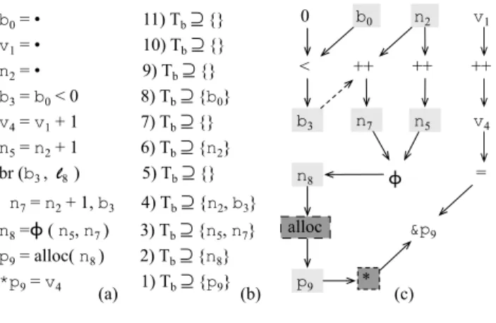
The integer primitive type has upper and lower bounds in many programming languages, including C, C++ and Java. Thus, there exist numbers that cannot be represented by these types. For instance, considering unsigned integers in C, if a number n is too large to fit into a primitive data type T , then n’s value wraps around, and n module Tmaxends up represented instead. In this case, Tmaxis the largest element in T . This phenomenon might invalidate our analyses. For instance, we can only assume that i < i + 1 if we know that i is not the maximum element in the integer type. To circum-vent this problem, we instrument every arithmetic operation that has an influence on memory allocation or indexing. We find this set of variables, which we shall call Tb, via the con-straints seen in Figure 8. These concon-straints use a points-to set Π : V 7→ 2V. If Π(v) = A, then A is the set of aliases of v, e.g., variables that contain addresses that might overlap any region pointed by v. We find Π via an instance of An-dersen’s style points-to analysis [3], augmented with Lazy Cycle Detection to improve scalability [17]. The constraints of Figure 8 determine a program slice [35]. If P is a pro-gram, then we say that P0 is a slice of P , with regard to the value of a certain variable v at point pc ∈ P , if P0correctly computes the value of v at pc. In our case, we are computing the union of all the slices containing variables used to either index, allocate or free memory. For instance, the constraint for v1= alloc(v2) puts v2into Tb, because any instruction

used to compute v2, the size of a memory block, must be

guarded against overflows.

We use the Sparse Evaluation Graph [12] to generate the constraints seen in Figure 8. The sparse evaluation graph of a SSA-form program contains one vertex for each of its vari-ables, and an edge from v to u if u is used in an instruction that defines v. These edges represent data dependences. We must also account for control dependences, as defined by Ferrante et al. [15, Def.1]. We say that a variable v controls a variable v0 if v is used on a branch, e.g., br(v, l), that de-termines if the instruction that defines v0executes or not. To handle control dependences, we do predication. An instruc-tion such as v = v0, p, means that v = v0has been predicated with all the variables in the set p. The set p is formed by all the variables that control the execution of v = v0.

We explore transitivity among predicates to avoid mark-ing an instruction with more than one predicate whenever possible. If we operate on SESE graph, e.g., control flow graphs that have the single-entry-single-exit property [15], then each instruction can be marked by only one predicate, due to transitivity. The CFGs of go-to free programs natu-rally produce SESE graphs. The backward slice defined in Figure 8 has a simple geometric interpretation. It determines the set of nodes, in the sparse evaluation graph, that can be reached from a backward traversal, starting from any instruc-tion that either defines or indexes a pointer.

free(v), p ⇒ Tb ⊇ {v} ∪ p v1= alloc(v2), p ⇒ Tb ⊇ {v2} ∪ p v = v1, p v = v1⊕ v2, p v = φ(v1, . . . , vn), p ⇒ v ∈ Tb Tb⊇ {vi} ∪ p ∗v1= v2, p ⇒          if Tb∩ Π(v1) = ∅ then Tb⊇ {v1} ∪ p else Tb⊇ {v1, v2} ∪ p v2= ∗v1, p ⇒          if v2∈ T/ b then Tb⊇ {v1} ∪ p else Tb⊇ {v1} ∪ p ∪ Π(v1) br(v, l), p ⇒ v ∈ Tb Tf ⊇ {p} other instructions ⇒ Tb ⊇ ∅

Figure 8. Constraints for the backward slice which finds the set Tb of variables to be sanitized against integer overflows. The analysis is parameterized by a points-to set Π.

Example 2 Figure 9 illustrates the graph-based view of the slice. The graph in Figure 9 (c) represents the dependences in the program of Figure 9 (a). All statements except line`8 are evaluated under a predication setp which is empty. In line`8,p = {b3} because this instruction is controlled by the value ofb3. Figure 9 (b) shows the constraints that we produce for this program, following the rules in Figure 8. Dark-grey boxes in Figure 9 (c) mark the origins of the backward slice; light-grey boxes mark the variables that are part of it. We must guard all the arithmetic operations that define these variables. The only operation that does not require instrumentation is the increment that defines variablev4 (it has no influence on memory allocation nor indexing).

Once we have the backward slice of variables Tb, we

guard every arithmetic instruction that defines variables in Tb against integer overflows. To achieve this goal, we use the instrumentation proposed by Dietz et al. [14], which is available for the LLVM compiler. We have configured this instrumentation to stop the program if an unwanted overflow happens. As we will show in Section 5, this instrumentation adds less than 2% of overhead to the transformed program.

Valid Uses of Integer Overflows. As shown by Dietz et

al. [14], overflows might be intentional in real-world pro-grams, and at least for unsigned integers this behavior is

b0 = • 11) Tb ⊇ {} v1 = • 10) Tb ⊇ {} n2 = • 9) Tb ⊇ {} b3 = b0 < 0 8) Tb ⊇ {b0} v4 = v1 + 1 7) Tb ⊇ {} n5 = n2 + 1 6) Tb ⊇ {n2} br (b3 , l8 ) 5) Tb ⊇ {} n7 = n2 + 1, b3 4) Tb ⊇ {n2, b3} n8 =ϕ ( n5, n7 ) 3) Tb ⊇ {n5, n7} p9 = alloc( n8 ) 2) Tb ⊇ {n8} *p9 = v4 1) T_b ⊇ {p₉} p₉ n8 n5 n7 b0 n2 v1 b3 v4 * alloc ++ ++ ++ < ϕ &p9 = 0 (a) (b) (c)

Figure 9. (a) Program that stores variable v4in memory. (b) Backward generation of set Tb. (c) Sparse Evaluation Graph. valid and defined by the C standard. The wraparound behav-ior can be used, for instance, in the implementation of hash-functions or pseudo-random generators, because it gives de-velopers a cheap surrogate for modular arithmetics. Our guards might change the semantics of the instrumented pro-gram, if this program contains legitimate uses of integer overflows in variables that are used to index or allocate mem-ory. We cannot distinguish an intentional use of an integer overflow from a bug. Thus, whoever uses our analyses must be aware that overflows are not allowed on any operation that might influence memory allocation or indexing. We believe that this requirement is acceptable for two reasons. First, en-suring the absence of this phenomenon in memory-related operations greatly improves the precision of our analyses. Secondly, we believe that the occurrence of integer over-flows in such operations is a strongly indication of a cod-ing bug. Our belief is backed by our empirical results: we have not found one single integer overflow in the memory-related operations used in SPEC CPU 2006. On the other hand, Dietz et al. have found over 200 occurrences of inte-ger overflows in SPEC CPU 2000, and Rodrigues et al. [26] have pointed out over 300 sites in SPEC CPU 2006 where overflows took place. We speculate that these overflows are not related to memory allocation or indexing.

Correctness of Integer Overflow Sanitiziation. We say

that Tbmodels P whenever Tbis a solution to the constraints seen in Figure 8, when applied on P . We can infer a number of interesting properties about Tb. Firstly, we know that the variables in Tbcontrol the list of allocated blocks, as we state in Theorem 4.1. Furthermore, we also know that Tbcontrols which positions of the memory heap are updated, as we state in that theorem. In other words, Tb does not determine the exact values stored in the heap, but it determines in which

heap cells these values go. In Theorem 4.1 we let c

∗_e

−−→ to denote a sequence of applications of the relation−→ that endc with one application of−→. These two relations have beene defined in Figure 5.

Theorem 4.1 Let S1 and S2 be two configurations of the memory stack of a program P , such that, for any v ∈ Tb,

we have that S1(v) = S2(v). For any pc, L and Q, we

have that, if (pc, S1, H, L, Q) c∗e −−→ (S0 1, H10, L01, Q01), and (pc, S2, H, L, Q) c∗e −−→ (S0 2, H20, L02, Q20), then: (i) L01=L02; (ii) For each addressi, H₁0[i] = ⊥ ⇔ H₂0[i] = ⊥, where H[i] = ⊥ if H[i] has not been assigned a value throughout

c∗e −−→.

Proof: We shall define a Memory Execution Trace (MET) as a sequence of instructions that contains any of free(v), v1 = alloc(v2), v2 = ∗v1, ∗v1 = v2or any assignment that defines a variable in Tb. Let’s denote the i-th instruction in a given MET M as M [i], and a subsequence within M as M [i : j]. A MET is a subsequence of instructions within the actual execution trace of a program. If E is an execution trace, we write that M ⊆ E. We shall prove that under the assumptions of the theorem, the two execution traces

generated by the stacks S1and S2encode the same METs.

We refer to these traces as E1 and E2, and to the METs

as M1and M2. The proof is by induction on the length of the METs. Henceforth, we assume that we are dealing with strict programs, i.e., programs in which variables are defined before being used. We assume that the property holds for any MET with n instructions, e.g., M1[1 : n] = M2[1 : n]. First, we prove that instructions at similar indices have the same opcode5_{; later, we prove that they read the same parameters.} Let’s assume that M1[n + 1] and M2[n + 1] have differ-ent opcodes. There are two cases to consider: either these in-structions are controlled by predicates with different values, or they are controlled by predicates with the same values. If we follow the first case, then there exists a branch br(v, l) that separates M1and M2, because v has different values in E1and E2. This separation, due to our induction hypotheses, happens after the execution of M1[n]. We know that v must have different values in E1and E2. We have that M1[n + 1] is controlled by a vector p of predicates, which includes v, by the definition of control dependence. A quick inspection of the rules in Figure 8 shows that these predicates are all placed in Tb, for any memory instruction. By the induction hypothesis, they must have the same values - a contradiction. If M1[n + 1] and M2[n + 1] are controlled by predicates with the same values, then, in compiler jargon, we say that these instructions are in the same basic block. Instructions within a basic block always execute in a fixed order. Thus, by the induction hypothesis, the first instruction that depends on any parameter defined in M1[1 : n] must be the same as the first instruction that depends on a value defined in M2[1 : n]. Let’s assume that M1[n + 1] and M2[n + 1] have the same opcodes. From this assumption, we proceed by case analysis on the possible shapes of M1[n + 1]:

5_{The opcode of an instruction denotes the operation that it represents.}

void read_matrix(int* data, char w, char h) { char buf_size = w * h; if (buf_size < BUF_SIZE) { int c0, c1; int buf[BUF_SIZE]; for (c0 = 0; c0 < h; c0++) { for (c1 = 0; c1 < w; c1++) { int index = c0 * w + c1; buf[index] = data[index]; } } process(buf); } } strlen(data) = 132char BUF_SIZE = 120_char = 0 0 0 0 0 1 1 0 = 6_char = 0 0 0 1 0 1 1 0 = 22_char = 1 0 0 0 0 1 0 0 = -124char w h h * w 1 2 3 4 5 6 7 8 9 10 11 12 13 14 buf_size = -124_char

Figure 10. A situation in which an integer overflow would invalidate our symbolic range analysis through a control dependence.

1. free(v): by induction, v is the same for M1[n + 1] and M2[n + 1], because it is in Tb, as Figure 8 shows. 2. v1 = alloc(v2): by induction, v2is the same for both

instructions, because it is in Tbaccording to Figure 8. 3. ∗v1= v2: by induction, v1is the same for both, because

it is in Tb

4. v2= ∗v1: by induction, v1is the same for both, because it is in Tb. Furthermore, any alias of v1is also in Tb, and by induction must contain the same values.

5. v = v1: by induction, v1is the same for both, because it is in Tb. The other types of assignments are treated in a similar way.

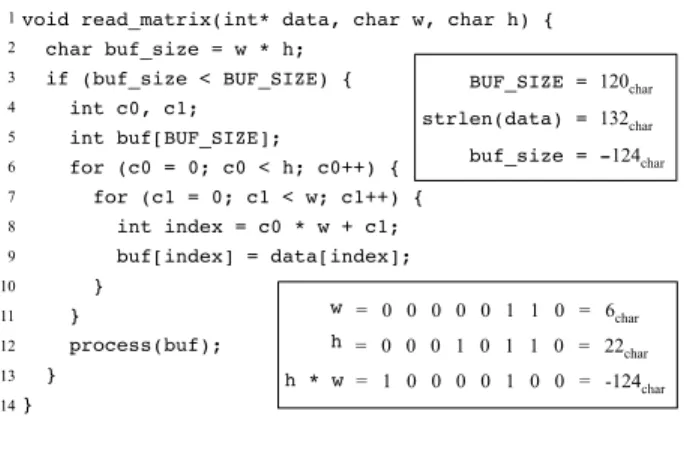
We would like to emphasize that handling control depen-dences is essential to ensure the correcteness of our analy-sis. This phenomenon might invalidate our analyses, as Fig-ure 10 illustrates. The function read matrix copies a trix, stored in linear format, to a buffer. The size of this ma-trix is expected to be given by the product of arguments w and h, which are eight-bit integers. If we have that w = 6 and h = 22, then w × h = −124, due to an integer over-flow. The test at line 3 would be true, but we would have “6 × 22 − 120 = 12” invalid accesses at line 9. Notice, in this case, there exists no direct data dependence between in-puts and memory indexing. An adversary can, nevertheless, force, through an integer overflow, a bad memory accesss, if we assume that variables w and h are part of the program’s input.

4.3 Symbolic Range Analysis

Range analysis, as originally defined by Cousot and Cou-sot [9], associates variables with integer intervals. This ap-proach enables several compiler optimizations, but it is not effective to validate memory accesses, as demonstrated by

Logozzo and F¨ahndrich [19]. The program in Figure 1 il-lustrates this deficiency. However, a traditional range anal-ysis will not find, in this program, constants onto which to rely upon, to prove that variables i and j only access valid positions of array p. To handle this program, we need a symbolic algebra expressive enough to lets us show that c0×w+c1 ≤ w×h, as long as 0 ≤ c0 < h and 0 ≤ c1 < w. To deal with the limitations of range analysis, we adopt the notion of symbolic ranges, originally defined by Blume and Eigenmann [5]. We define the symbolic kernel of a pro-gram as the set formed by either constants known at com-pilation time, or variables defined as input values, such as the formal parameters of functions. Henceforth, we will use the general term symbol to denote a variable in a symbolic kernel. In this paper, elements of the symbolic kernel are produced by read operations, e.g., v = •, or load opera-tions, as we do not keep track of values in memory. We use the abstract interpretation framework [9] in order to gener-ate invariants as symbolic ranges over the symbolic kernel of the program. Basically, we will extract a set of (interval) constraints from the program, and then perform a fixpoint algorithm until convergence. The result will be an upper ap-poximation of “actual values” of the program variables, in all possible execution of the program.

Symbolic expressions We say that E is a symbolic

expres-sion, if, and only if, E is defined by the grammar below. In this definition, s is a symbol and n ∈ N.

E ::= n | s | min(E, E) | max(E, E) | E − E

| E + E | E/E | E mod E | E × E We shall be performing arithmetic operations over the

partially ordered set S = SE∪{−∞, +∞}, where SEis the

set of symbolic expressions. The partial ordering is given by −∞ < . . . < −2 < −1 < 0 < 1 < 2 < . . . + ∞. There exists no ordering between two distinct elements of the symbolic kernel of a program. To define the ordering between two expressions we need the notion of the valuation of a symbolic expression. If M : s 7→ Z is a map of symbols to numbers, then we define the value of E under M as (M, E) = n, n ∈ Z. The integer n is the number that we obtain after substituting symbols in E by their values in M . To obtain a valuation (E) of a symbolic expression E, we replace its symbols by numbers in Z. We say that E1< E2 if any valuation of both E1and E2under any map M always gives us (M, E1) < (M, E2).

Lattice of symbolic expression intervals A symbolic inter-valis a pair R = [l, u], where l and u are symbolic expres-sions. We denote by R↓the lower bound l and R↑the upper bound u. We define the partially ordered set of (symbolic) intervals S2 = (S × S, v), where the ordering operator is defined as: [l0, u0] v [l1, u1], if l1≤ l0∧ u1≥ u0 v = • ⇒ R(v) = [v, v] v = o ⇒ R(v) = R(o) v = v1⊕ v2 ⇒ R(v) = R(v1) ⊕IR(v2) v = φ(v1, v2) ⇒ R(v) = R(v1) t R(v2) other instructions ⇒ ∅ t = a < b br (t, l) at = σ(a) bt = σ(b) af = σ(a) bf = σ(b) l

R(at ) = [R(a)↓, min(R(b)↑− 1, R(a)↑)]

R(bt ) = [max(R(a)↓ + 1, R(a)↓), R(b)↑]

R(af ) = [max(R(a)↓, R(a)↑), R(a)↑]

R(bt ) = [R(b)↓, min(R(a)↑, R(b)↑)]

Figure 11. Constraints for the symbolic range analysis We then define the semi-lattice SymBoxes of symbolic in-tervals as (S2, v, t, ∅, [−∞, +∞]), where the join operator “t” is defined as:

[a1, a2] t [b1, b2] = [min(a1, b1), max(a2, b2)] Our lattice has a least element ∅, so that:

∅ t [l, u] = [l, u] t ∅ = [l, u] and a greatest element [−∞, +∞], such that:

[−∞, +∞] t [l, u] = [l, u] t [−∞, +∞] = [−∞, +∞] Clearly, this lattice is infinite; therefore, in order to end up the computation of the set of constraints we use a widening operator defined by (under the assumption R1v R2):

R1∇R2= [l, u], where          l = R1↓ if R1↓= R2↓ l = −∞ otherwise u = R1↑ if R1↑= R2↑ u = +∞ otherwise

This is the extension of the classical widening on intervals to symbolic intervals. Like the classical widening on interval, a lower (resp. upper) bound of a given symbolic interval can only be stable or diverge towards −∞ (resp +∞), thus our widening operator will ensure the convergence of our analysis.

Abstract interpretation on the E-SSA form. To apply the

abstract interpretation framework, we also have to give an interpretation of the operations of the program. This is done in Figure 11.

•assigments after reads give only symbolic information.

•assigments to expressions causes the expression to be

- [l0, u0] +I[l1, u1] = [l0+ l1, u0+ u1] - [l, u] +I_{∅ = [l, u]}

- [l0, u0] ×I [l1, u1] = [min(T ), max(T )], where T = {l0× l1, l0× u1, u0× l1, u0× u1}

- [l, u] ×I_{∅ = [l, u]}

Figure 12. Range Computation library

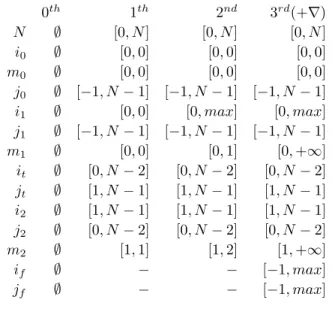
0th ₁th ₂nd ₃rd_(+∇) N ∅ [0, N ] [0, N ] [0, N ] i0 ∅ [0, 0] [0, 0] [0, 0] m0 ∅ [0, 0] [0, 0] [0, 0] j0 ∅ [−1, N − 1] [−1, N − 1] [−1, N − 1] i1 ∅ [0, 0] [0, max] [0, max] j1 ∅ [−1, N − 1] [−1, N − 1] [−1, N − 1] m1 ∅ [0, 0] [0, 1] [0, +∞] it ∅ [0, N − 2] [0, N − 2] [0, N − 2] jt ∅ [1, N − 1] [1, N − 1] [1, N − 1] i2 ∅ [1, N − 1] [1, N − 1] [1, N − 1] j2 ∅ [0, N − 2] [0, N − 2] [0, N − 2] m2 ∅ [1, 1] [1, 2] [1, +∞] if ∅ − − [−1, max] jf ∅ − − [−1, max]

Figure 13. Symbolic range analysis in program of Figure 6

•φ functions are “join nodes”, thus we perform a

(sym-bolic) interval union.

•On intersection nodes (tests), we perform a (symbolic)

interval intersection.

We solve the system of contraints using a Kleene iter-ation on the system of constraints. The analysis is sparse since we do not need the control points any more. The in-formation is only attached to variables. Widening is applied on a φ node only after 3 iterations of symbolic evaluation (“delayed widening”). This decision is arbitrary, and a larger number of iterations might increase the precision of our re-sults. However, in our experiments we only observed very marginal gains by using more iterations.

Example 1 (continuing from p. 2) Figure 13 shows the steps that our analysis performs on the program of Figure 6. The order in which we evaluate constraints is given by the re-verse post-ordering of the program’s control flow graph. This ordering tends to reduce the number of iterations of our fixed point algorithm [23, p.421]. However, any order of evaluation would led to the same result. In this example, we let “max” be max(0, N − 1).

On the evaluation of symbolic expressions. As shown

in the preceeding paragraphs, we have to evaluate symbolic

expressions (simplification of expressions like max(e1, e2), equality tests, . . . ). We rely on GiNaC [4], a library for symbolic manipulation, to perform these operations6. For the equality test, if GiNaC is not able to prove a given equality between symbolic expressions, we conservatively assume that the two expressions are not comparable. As a consequence, we may widen an expression to +∞ even if it was stable.

Correctness of the Symbolic Range Analysis. Abstract

values of the SymBoxes domain are functions R that asso-ciate to each variable v of the program a symbolic interval. The concretisation of a given symbolic range is the set of valuations (variables and symbols) that satisfy the induced constraints:

γSymBoxes (R) =

{(σ, M ), σ valuation of variables and M valuation of symbols s.t. ∀v ∈ V, (M, R(v)_↓) ≤ σ(v) ≤ (M, R(v)_↑)}

Here the union of the valuations σ and M corresponds to the stack (S) defined in the semantics of the core language (Figure 5). The order of application of σ and M does not matter.

Theorem 4.2 The former analysis always returns an over-approximation of the actual ranges of the variables of the program (no matter the valuations of the symbols would be). Proof: The abstract interpretation framework implies that any valuation of the variables and symbols of the program (Stack) belongs to the concretisation of the intervals that our analyses finds (γSymBoxes (R)).

4.4 Symbolic Region Analysis

As we mention in Section 6, the vast majority of previous algorithms to eliminate array bound checks have been de-signed for the Java programming language. In Java, arrays are associated with their sizes, and this information is avail-able at runtime. In other words, Java programs often uses the array.length attribute to iterate over an array, and we can rely on the semantics of this field to eliminate more access guards. In C, arrays are not packed together with size infor-mation. We have to infer this size automatically. To solve this problem, we resort to static analysis. We have designed a novel region analysis, which binds each pointer to an in-terval of valid offsets.

Our analysis of regions rests on the semi-lattice SymRegion (S2, v, u, [−∞, +∞], ∅), which is the inverse of the struc-ture used in the symbolic range analysis of Section 4.3. Here, we have a meet operator “u”, such that:

[a1, a2]u[b1, b2] = (

∅, if a2< b1or b2< a1

[max(a1, b1), min(a2, b2)], otherwise

v1 = alloc(n) v1 v2 = v1 + 1 W(v1) = [0, n − 1] v2 W(v2) = [−1, n − 2] v3 = v1 + n v2 W(v3) = [−n, −1] n

Figure 14. Semantics for “valid offsets” The least element of our semi-lattice is ∅, so that:

∅ u [l, u] = [l, u] u ∅ = ∅

And the greatest is [−∞, +∞], which we define as follows: [−∞, +∞] u [l, u] = [l, u] u [−∞, +∞] = [l, u] Therefore, whereas in Section 4.3 we were always expand-ing ranges, here we are always contractexpand-ing them. In other words, the symbolic range analysis finds the largest ranges covered by variables, i.e., it is a may analysis. On the other hand, the symbolic region analysis finds the narrowest re-gions that pointers can dereference, i.e., it is a must analysis. In the abstract interpretation jargon, we say that we are com-puting under-approximations.

Like the symbolic range analysis from Section 4.3, the region analysis also associates with each variable an stract state given by an interval. However, here this ab-stract state has a very different interpretation. If we say that W (p) = [l, u], then we mean that all the addresses between the offsets p+l and p+u are valid. Figure 14 clarifies this se-mantics. The first instruction of Figure 14 allocates n words in memory, and assigns the newly created region to pointer v1. Thus, given a stack S, if b1 = S(v1) is the value of v1, then any address between b1+ 0 and b2+ n − 1 is valid. The second instruction increments v1, and calls the new ad-dress v2. Similarly, if b2= S(v2), then the address b2− 1 is valid, and the address b2− n − 2 is also valid. As we state in Theorem 4.3, it is always safe to dereference a pointer if it includes the address zero among its valid offsets.

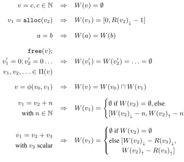
We describe an instance of region analysis as a set of con-straints. These constraints are extracted from the program’s source code, according to the rules in Figure 15. The figure naturally distinguish between scalars and pointers. Pointers are variables that have been initialized with the alloc in-struction, or that are computed as functions of other point-ers. Scalars are all the other variables; hence, they are always bound to the region ∅. For the last constraint, we must en-code the fact that we cannot add a pointer and a variable, thus v3must be a scalar. Therefore, if p1is defined as p1= p2+v, then its region is given by the admissible region of p2 ad-dressed with all the possible values of v. That is why we must consider the interval range of v. Before moving on, we draw the reader’s attention to the abstract semantics of the free(v) instruction. As we explained in Section 4.1, this in-struction leads us to rename every alias of v, so that all of these new names will be bound to the new region ∅.

v = c, c ∈ N ⇒ W (v) = ∅ v1= alloc(v2) ⇒ W (v1) = [0, R(v2)_↓− 1] a = b ⇒ W (a) = W (b) free(v); v01= 0; v 0 2 = 0 . . . v1, v2, . . . ∈ Π(v) ⇒ W (v10) = W (v 0 2) = . . . = ∅ v = φ(v0, v1) ⇒ W (v) = W (v0) u W (v1) v1= v2+ n with n ∈ N ⇒ W (v1) = ( ∅ if W (v2) = ∅, else [W (v2)↓− n, W (v2)↑− n] v1= v2+ v3 with v3scalar ⇒ W (v1) =      ∅ if W (v2) = ∅ else [W (v2)↓− R(v3)↓, W (v2)↑− R(v3)↑]

Figure 15. Constraint generation for the symbolic region analysis.

Our region analysis uses a widening operator for φ-functions, to ensure that our algorithm terminates in face of pointer arithmetics. Because this operator reduces ranges, it is called a lower widening 7 _{, under the terminology of} [21]. This operator is defined as follows:

R1∇R2=

(

∅ if R2↓> R1↓or R2↑< R1↑

R2 otherwise

Example 1 (continuing from p. 2) If we run our region analysis on the program of Figure 6, then we get that W (p) = [0, N − 1], W (pi) = [0, 1], W (pj) = [−1, 0],

andW (pm) = [0, −∞] = ∅. These ranges correctly tells

us, for instance, that the largest (safely) addressable offset from addressp is N − 1.

Example 3 Figure 16 shows how widening ensures that our region analysis converges. This program implements a typ-ical character search in a string, e.g., for(v = p; p != ’0’; p++). In this example we have widened after p1, the variable defined by aφ-function, had changed twice. After widening we reach a fixed-point in the third round of ab-stract interpretation.

Example 1 (continuing from p. 2) The ranges that we find for the program in Figure 6 let us remove bound-checks for

the memory accesses at lines 18 and 20. The region ofpi

tells us thatpiandpi− 1 are safe addresses. The region of pj indicates thatpjandpj+ 1 are also safe addresses. On

7_{Let us point out the fact that, unlike the proposition of [21], we directly}

p1 = φ(i0, it) x = *p1 t = x '\0' br (t, l) p2 = p1 + 1 v = alloc(N) pe = v + N p0 = v v pe p0 p1 0th 1st 2nd ∇ p2 [0, N−1] [−N, −1] [0, N−1] [0, N−1] [−1, N−2] [−∞, +∞] [−∞, +∞] [−∞, +∞] [−∞, +∞] [−∞, +∞] [0, N−1] [−N, −1] [0, N−1] [0, N−2] [−2, N−3] 3rd [0, N−1] [−N, −1] [0, N−1] ∅ [−2, N−3] [0, N−1] [−N, −1] [0, N−1] ∅ ∅

Figure 16. An example where we have used widening to ensure that region analysis converges.

the other hand, the range ofpmtells us that it is not safe to dereference this pointer without a bound-check. In this case, we have a false-positive, because we conservatively assume that a memory access is unsafe.

Correctness of the Symbolic Region Analysis. Abstract

values of the SymRegion domain are functions W that asso-ciate to each variable p a symbolic interval. The concretisa-tion of W is the set of tuples (S, H, L) (program context) which correspond to adresses in the ranges [pi+ `i, pi+ ui] : γSymRegion (W ) = {(S, H, L, Q) such that ∀p ∈ V, ∀α,

if H(S(p) + S(W (p))_↓)) ≤ α ≤ H(S(p) + S(W (p)_↑)))

then inBlock(L, α)}

Theorem 4.3 states the key property of our symbolic region analysis. We have defined the theorem for loads, but it is also true for instructions such as ∗v1= v2, which store the contents of v2into the address pointed by v1.

Theorem 4.3 Let P be a program and pc ∈ N, such that P [pc] is v2= ∗v1. If0 ∈ W (v1), then P cannot be stuck at pc.

Proof: (Sketch) The abstract interpretation framework im-plies that our concretisation is a subset of the actual valid addresses in L. Thus 0 ∈ W (v1) garanties that v1is a valid address.

4.5 Tainted Flow Analysis

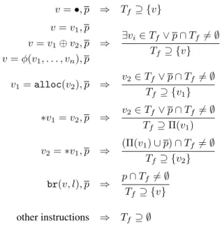
We have included an optional tainted flow analysis in our framework. If we are interested in preventing only buffer overflows caused by malicious inputs, then we can restrict our attention to operations that are influenced by values pro-duced by external functions. To illustrate this observation, we use Figure 17. Figure 17 (a) shows a program that reads two values, m and n and use them to control the writing of an array v. Variable n controls the maximum extension of the array that is written. If this variable is larger than the size of the array, bad memory accesses will take place. The variable

(a) m = read(); n = read(); int i = 0; for (; i < n; i++) { if (i % m) v[i] = 0 } 1 2 3 4 5 6 7 i0 i i1 v p0 p₁ m n 0 ϕ dec inc = 0 % (c) (d) _T f = { m, p0, Π[v], n, p1, i1, i } l0: end l5: m = • n = • i0 = 0 i =ϕ (i0, i1) p0 = n − 1 br (p0, l3) p₁ = i % m, p₀ br (p1, l4) *v = 0, p₁ i1 = i + 1, p1 jmp l2 l1: _l 2: l3: l4: (b) * &v

Figure 17. (a) Program containing implicit tainted flow that could cause out-of-bounds access. (b) Intermediate repre-sentation. Predicates propagating implicit information are shown in gray. (c) Dependence graph. Control flow edges are dashed. (d) Tainted set Tf.

n is part of the input of the program; hence, we assume that it can be controlled by a malicious user. By feeding the pro-gram with a large value of n, this user can cause an invalid access at line 6 of Figure 17 (a). Our taint analysis identifies which memory accesses can be manipulated by malicious users, in such a way that the other accesses do not need to be guarded. Our tainted flow analysis considers the following set of external functions:

•functions not declared in any file that is part of the com-piled program;

•functions without a body;

•functions that can be called via pointers.

The idea behind this tainted flow analysis is as follows: we want to instrument stores, loads and memory allocations that might be controlled by external sources of data. In this case, we are assuming that every source of external data is untrusted.

Tainted flow analysis has been discussed exhaustively in the literature [28]; thus, it is not a novel contribution of this

v = •, p ⇒ Tf ⊇ {v} v = v1, p v = v1⊕ v2, p v = φ(v1, . . . , vn), p ⇒ ∃vi∈ Tf∨ p ∩ Tf 6= ∅ Tf ⊇ {v} v1= alloc(v2), p ⇒ v2∈ Tf ∨ p ∩ Tf 6= ∅ Tf ⊇ {v1} ∗v1= v2, p ⇒ v2∈ Tf ∨ p ∩ Tf 6= ∅ Tf ⊇ Π(v1) v2= ∗v1, p ⇒ (Π(v1) ∪ p) ∩ Tf 6= ∅ Tf ⊇ {v2} br(v, l), p ⇒ p ∩ Tf 6= ∅ Tf ⊇ {v} other instructions ⇒ Tf ⊇ ∅

Figure 18. Constraints for the forward slice which finds the set Tf of variables that are influenced by input values. The analysis is parameterized by a points-to set Π.

work. We run tainted flow analysis on the same dependence graph that we have used to implement our integer overflow slice from Section 4.2. Therefore, the tainted flow analysis determines a slice in the program dependence graph, which handles both implicit and explicit flows of information. The differences from the analysis of Section 4.2 are as follows:

•The tainted flow analysis is a forward slice of the pro-gram. The overflow analysis is a backward slice.

•The sources of the tainted flow slice are the instructions that use values produced by external sources. The sources of the integer overflow slice are the memory operations.

•The sinks of the tainted flow slice are memory accesses. The sinks of the overflow slice are integer arithmetic operations.

Like the other algorithms from Section 4, our tainted flow analysis is sparse. We also track control dependences be-tween branches and instructions through predication. As an example, Figure 17 (b) shows how each instruction of a pro-gram is predicated. Notice that we only have to predicate the instructions in block l4with p1, and not with p0and p1, due to transitivity: p0 already predicates p1. Such transitivities are discovered using Ferrante et al.’s techniques [15]. The sparse evaluation graph in Figure 17 (c) shows the control dependence edges that this predication generates. Hence it associates with the entire live range of a variable one of two states: tainted or clean. Memory accesses that are indexed only by clean variables do not need to be guarded against overflows. The other accesses will still be analyzed by our other algorithms of Section 4, and only if our symbolic

anal-yses cannot prove that they are safe, we will have to maintain bound-checks.

The forward flow analysis given in Figure 18 builds the set Tf of tainted variables. Like the backward analysis of Section 4.2, this analysis is parameterized by a points-to set

Π : V 7→ 2V_{. If P is a program, and T}

f is the taint set produced by our analysis, then we say that Tfmodels P . The set Tffor our example is given in Figure 17. We use a lattice with two elements: either a variable is tainted, in which case it belongs to Tf, or it is clean. Therefore, our taint analysis reduces to traditional program slicing [33], which we solve via graph traversal, as Figure 17(c) illustrates. Theorem 4.4 states the key non-interference property of our tainted flow analysis.

Theorem 4.4 Let Q1andQ2be two input queues, such that,

for some pc, S, H and L we have (pc, S, H, L, Q1)

c∗e −−→ (S1, H1, L1, Q01), and (pc, S, H, L, Q2)

c∗e

−−→ (S2, H2, L2, Q0₂). For any variable v, such that v /∈ Tf, we have that S1(v) = S2(v).

Proof: (Sketch) This proof is similar to the proof of The-orem 4.1, and so we omit its details. We need the notion of an Input Execution Trace, which is formed by all the instruc-tions that define variables in Tf. The proof follows by induc-tion on the length of these traces, alongside case analysis on the Rules seen in Figure 18.

4.6 Inter-procedural Analysis

All the analyses that we describe in this paper are inter-procedural; albeit context-insensitive for the sake of scala-bility, as we do not consider the state of the function stack when analyzing calls. To analyze a program, we visit func-tions in an order defined by its call-graph. This graph con-tains a vertex for each function, and an edge from function f to function g if f contains a call to g among its instruc-tions. We visit functions following a depth-first traversal of the program’s call graph. If the program does not contain re-cursive calls, then its call-graph is a directed acyclic graph. In this case, the depth-first traversal, starting from main, the entry point of a C program, gives us the topological ordering of functions. In other words, we only visit a function f after we have visited any function that calls f . As we will explain shortly, this ordering lets us compute all the information that we need to analyze a function, before visiting the function itself. On the other hand, it forces us to assume that values returned from functions are always part of the symbolic ker-nel, as we have no information about them.

After we analyze the body of a function g, we have enough information to compute a “Less-Than” relationship between variables declared in its body. We compute such relationship for every pair of variables that are used as actual parameters of other functions called in the body of g. Let f (v1, v2, . . . , vn) be an instruction, within the body of g, that calls a certain function f with actual parameters vi, 1 ≤ i ≤ n. We determine the “Less-Than” relation between

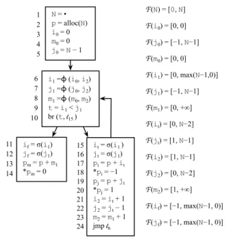
void keep(int *s, int i_s, int N_s, int* d, int i_d, int N_d){ int x = 0; if (i_s < N_s) { x = s[i_s]; } if (i_d < N_d) { d[i_d] = x; } } int main() { unsigned N_x = •; unsigned N = N_x + 1; int* p = alloc(N); unsigned N_y = •; unsigned N₀ = N_y + 1; int* p₀ = alloc(N₀); keep(p₀, 0, N₀, p, 0, N) unsigned N₁ = 4; int* p₁ = alloc(N₁); keep(p₁, 1, N₁, p, 1, N) } p₀ 0 N₀ p 0 N p₀ = > < ? > ? 0 < = < < = < N₀ > > = ? > ? p ? > ? = > < N ? > ? > > = 0 < = < < = < p₁ 0 N₁ p 1 N p₁ = > < ? > ? 1 < = < < < < N₁ > > = ? > ? p ? > ? = ? < N ? > ? > ? = 1 ? > ? ? = ? W(d) = [0, d] R(i_d) = [0, 1] R(N_d) = [0, d + 1] (b) (c) (a) R(i_s) = [0, s] W(s) = [0, s + 1] R(N_s) = [0, s + 2] 1 2 3 4 5 6 7 8 9 10 11 12 13 14 15 16 17 18 19 20 21 22

Figure 19. Example of inter-procedural analysis. (a) Sym-bolic bounds of formal parameters. “Less-than” analysis on the actual parameters of (b) first call to keep, and (c) second call to keep.

each vi, vj, 1 ≤ i, j ≤ n. Additionally, we also determine minimum lower bounds to all the scalar variables vi.

We implement the less-than check differently, depend-ing on the actual parameters bedepend-ing pointers or scalars. Our less-than test between scalars viand vj amounts to check-ing if R(vj)_↑ < R(vi)↓. If vi is a pointer, then we check if R(vj) ⊆ W (vi). We perform these checks through GiNaC, the same library that we mentioned in Section 4.3. We have augmented GiNaC with operations to handle inequalities in-volving the symbols min and max, because these expressions are part of our framework, and did not exist originally in that library. To determine the lower bounds of a formal parameter vi that is a scalar, we compute the minimum among all the actual instances of vi. Example 4 illustrates our technique. Example 4 Figure 19 shows how we handle function calls. In the figure, we have two calls of keep. Each call generates different “less-than” relationships, which we show in part (b) and (c) of the figure. We use the question mark to indicate that we do not know size relation between two variables.

To propagate information computed for actual parameters to formal parameters we use a simple meet operator. Let f1(v11, . . . , v1n), . . . , fm(vm1, . . . , vmn) be all the calls of a function f throughout a program P , and let f (v1, . . . , vn) be the declaration of f in P . If, for every call, we have that vij < vik, 1 ≤ j, k ≤ n, 1 ≤ i ≤ m, then we let vj < vk when analyzing f . Each viis part of the symbolic kernel of f , thus, these variables are assigned to symbolic bounds. To determine these bounds, we sort all the formal

parameters viaccording to the Less-Than relation. We call a sequence of variables sorted in this way a Less-Than Chain. If vi is the first, i.e., smallest, variable in such a chain, we let its bound to be R(vi) = [min(vki), s], where min(vki) is the minimum bound among all the actual parameters vki, and s is a fresh symbol. If vi is a pointer, then we let its region be W (vi) = [0, s]. If vjis the second element in this chain, we let its range to be R(vj) = [min(vkj), s + 1], and so on. In the presence of recursion we initialize all the formal parameters of mutually recursive functions with fresh symbols, without implementing the less-than check. Example 4 (continuing from p. 14) Figure 19 (a) gives the symbolic states - ranges and regions - of all the formal parameters of function keep. We have two less-than chains in this program:(is, s, Ns) and (d, Nd). The first chain leads us to initialize the symbolic bounds ofis, s and Ns with s, s + 1 and s + 2 respectively.

Discussion: our approach is different than the traditional way to implement a context-insensitive inter-procedural analysis. Before initializing the abstract state of a formal parameter vi, the traditional approach joins the state of all the actual parameters vki, and copies this state to vi, fol-lowing the technique that Nielson et al call the naive inter-procedural analysis[23, p.88]. This is what we do in the ab-stract interpretation of φ-functions, as defined in Figures 11 and 15. However, when analyzing function calls, we change information, before performing the naive propagation. In-stead of doing a join of symbolic ranges, we join less-than relations. We believe that our approach is better than the naive inter-procedural method, as we explain in Example 4. Example 4 (continuing from p. 14) Had we performed a naive join of abstract states in Figure 19, we would have gottenR(is) = [0, 0] t [1, 1] = [0, 1], and W (s) = W (p0) u W (p1) = [0, min(Ny+ 1 − 1, 4 − 1)] = [0, min(Ny, 3)]. Given that we do not know thatNy > 1, we would not be able to prove that the memory access at line 4 is always safe. Our less-than relations let us deal with this shortcoming of the naive approach.

4.7 Implementation details

We have combined the three static analyses of Section 4 into a framework that we call GreenArrays. Figure 20 shows how these analyses are organized. The tainted flow analysis, which we have described in Section 4.5, is optional. As we show in Section 5, it increases by a small margin the number of bound checks that we can eliminate.

GreenArrays works on top of AddressSanitizer. Address-Sanitizer is an extension of the well-known LLVM com-piler [18], that produces memory safe binaries out of C programs. This tool relies on a modified memory alloca-tion library that generates enough meta-informaalloca-tion to sup-port runtime access checks. AddressSanitizer shadows every chunk of memory that it allocates. At runtime, each memory