École Normale Supérieure
Computer Science Department
Internship Report
Checking the type safety of rewrite rules in λΠ-calculus modulo
rewriting
Wu Jui-Hsuan
supervised by
Frédéric Blanqui
12& Valentin Blot
12 1INRIA2ENS Paris-Saclay
1 Introduction
Lambdapi is a new proof assistant based on the λΠ-calculus modulo theory [5], which extends the simply typed lambda calculus with dependent types and an equivalence relation on types generated by user-defined rewrite rules. The expressiveness of rewriting allows to formalize proofs that cannot be done in other proof assistants. However, as Lambdapi is based on the propositions-as-types inter-pretation, one should verify that the system satisfies the subject reduction property before starting to construct proofs within it. During my internship, I studied a new algorithm proposed by F. Blanqui for checking type preservation of rewrite rules and implemented it in Lambdapi. Besides, in order to improve the unification (modulo rewriting) procedure, I designed an algorithm for checking injectivity of function symbols.
2 λΠ-calculus modulo
2.1 λΠ-calculusThe λΠ-calculus is an extension of the simply typed lambda calculus (λ→) with dependent types. In this calculus, we introduce a particular type T ype and ”types” in λ→ are just terms of type T ype in the λΠ-calculus. Some terms have the type A→ T ype, where A is of type T ype, and can be applied to a term t of type A to build a type depending on t. Besides, a type Kind is introduced as the type of terms T ype, A→ T ype, etc. Finally, the usual arrow A → B is extended to the dependent product Πx : A.B to handle the possible dependency of the type B on the type A.
We writeS for the set of sorts {T ype, Kind} and we assume given a set X = {x, y, z, · · · } of variables and a setF of function symbols.
Then we can define the set T of terms of the λΠ-calculus.
Definition 2.1. (Term) The set of terms in the λΠ-calculus is given by:
t := x| s | f | tt | λx : t.t | Πx : t.t, where x ∈ X , s ∈ S and f ∈ F
We then assume that each function symbol f is equipped with a type τ (f ) and a sort s(f ). If
τ (f ) = Πx1 : T1.· · · .Πxn: Tn.U where U is not a product, then f is said of arity n. In fact, function
symbols can be regarded as variables declared in a global context (”signature”) of the system. We now present the typing rules of the λΠ-calculus:
Well-formedness of the empty context
[ ] well-formed
Declaration of a variable Γ⊢ A : s
s∈ S
Γ, x : A well-formed
T ype is of type Kind
Γ well-formed Γ⊢ T ype : Kind Variable Γ well-formed x : A∈ Γ Γ⊢ x : A
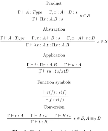
Product Γ⊢ A : T ype Γ, x : A⊢ B : s s∈ S Γ⊢ Πx : A.B : s Abstraction Γ⊢ A : T ype Γ, x : A⊢ B : s Γ, x : A⊢ t : B s∈ S Γ⊢ λx : A.t : Πx : A.B Application Γ⊢ t : Πx : A.B Γ⊢ u : A Γ⊢ tu : (u/x)B Function symbols ⊢ τ(f) : s(f) ⊢ f : τ(f) Conversion Γ⊢ t : A Γ⊢ A : s Γ⊢ B : s s∈ S, A ≡βB Γ⊢ t : B
Fig. 1. Typing rules of the λΠ-calculus.
We have the uniqueness (modulo ≡β) of types in λΠ-calculus.
Proposition 2.1. For all Γ, t, A, B, if Γ⊢ t : A and Γ ⊢ t : B, then A ≡β B. 2.2 λΠ-calculus modulo rewriting
The λΠ-calculus modulo rewriting is an extension of the λΠ-calculus with a set R of rewrite rules. Let
≡ be the minimal congruence that contains R and β-conversion. The typing rules of the λΠ-calculus
modulo R can be obtained from those of the λΠ-calculus by replacing ≡β with ≡ in the conversion rule.
Notation 2.1. In the following, we denote the smallest congruence containing a relation S by≡S. 2.3 Lambdapi
2.3.1 Metavariables
In Lambdapi, we extend the λΠ-calculus modulo by introducing metavariables which are used to rep-resent yet unknown term. We denote byM the set of metavariables.
t :=· · · | M where M ∈ M
We now define the types of metavariables and the algebraic fragment of Lambdapi. Each metavariable M is equipped with a type tM, with some contraints explained below.
The type of a yet unknown object-level term is also yet unknown, but the type of this type should be a sort. We distinguish thus object-level metavariables and type-level metavariables:
Definition 2.2.
• An object-level metavariable is a metavariable M s.t. tM is a type-level metavariable.
• A metavariable is either a type-level metavariable or an object-level metavariable.
• We denote by M0 the set of object-level metavariables and by M eta(t) the set of object-level
metavariables occurring in t.
The algebraic fragment of the terms of Lambdapi corresponds to the terms of first-order rewriting:
Definition 2.3. Let A0be the smallest set of terms such that M0⊆ A0, and f a1· · · an∈ A0 for all f ∈ F, a1,· · · , an∈ A0. The setA of algebraic terms is defined as A0− M0
We now define substitutions.
Definition 2.4. (substitutions) A substitution σ is a map assigning to each metavariable M a term.
Its application to a term is defined as follows: • xσ = x for x∈ X • f σ = f for f ∈ F • (tu)σ = (tσ)(uσ) • (λx : A.t)σ = λx : Aσ.tσ • (Πx : A.t)σ = Πx : Aσ.tσ • M σ = σ(M )
• We define the domain dom(σ) of a substitution σ as the set{M ∈ M | Mσ ̸= M}.
2.3.2 Type inference and type checking
The type inference relation of Lambdapi is the same as that of the λΠ-calculus modulo rewriting. Note that, if a term contains a metavariable, then it is not typable.
Since metavariables are used to represent unknown terms in a term t, one might want to infer the constraints on terms replacing the metavariables of t that need to be satisfied to make the term t typable.
We now present the constraint-generating type inference and type checking algorithm for algebraic terms, consisting of the following judgement forms.
Γ⊢ t ↑ A[E] type checking Γ⊢ t ↓ A[E] type inference Note that we add a special field E which contains a set of constraints.
Function applications τ (f ) = Πx1: A1.· · · .Πxn: An.U ∀i ∈ {1, · · · , n}, ⊢ ti ↑ Ai[Ei] ⊢ ft1· · · tn↓ (t1/x1,· · · , tn/xn)U [ ∪ 1≤i≤nEi] Object-level metavariables ⊢ M ↑ T [{(tM, T )}]
Type checking of function applications
⊢ ft1· · · tn↓ A[E] ⊢ ft1· · · tn↑ B[E ∪ {(A, B)}]
Fig. 2. (Constraint-generating) type inference and type checking algorithm for algebraic terms. Proposition 2.2.
1. If t is an algebraic term, then there exists at most one (E, A) such that⊢ t ↓ A[E].
2. If t is an algebraic term or an object-level metavariable, then for all term A, there exists at most one E such that ⊢ t ↑ A[E].
Remark 2.1. The proposition above guarantees the existence of two algorithms Inf erT ype and
CheckT ype that correspond to the type inference and the type checking respectively.
Definition 2.5. We say that a substitution σ satisfies a set E of equations, written σ|= E, if for all
(a, b)∈ E, aσ ≡ bσ.
Definition 2.6. We say that a substitution σ′ is a type-level extension of another substitution σ if
M σ′= M σ for all M ∈ dom(σ) and dom(σ′)− dom(σ) ⊆ {tM | M ∈ M0∩ dom(σ)}.
Theorem 2.1. Suppose that⊢ t ↑ T [E] (or ⊢ t ↓ T [E]). Let σ be a substitution. Then we have:
1. (σ|= E and ∀M ∈ Meta(t), Γ ⊢ Mσ : tMσ)⇒ Γ ⊢ tσ : T σ.
2. Γ ⊢ tσ : V ⇒ there exists a type-level extension σ′ of σ s.t. V ≡ T σ′, σ′ |= E and ∀M ∈ M eta(t), Γ⊢ Mσ′: tMσ′).
Proof. By induction on the derivation of⊢ t ↓ T [E] (or ⊢ t ↑ T [E])
• (Function applications)
1. Suppose that σ |= ∪1≤i≤nEi and ∀M ∈ Meta(ft1· · · tn), Γ ⊢ Mσ : tMσ. We have, ∀1 ≤ i ≤ n, σ |= Ei and ∀M ∈ Meta(ti), Γ⊢ Mσ : tMσ. By I.H.,∀i ∈ {1, · · · , n}, Γ ⊢ tiσ : Aiσ = Ai (the Ai’s and U contain no metavariable since function symbols are declared in
the global context). Hence, Γ⊢ (ft1· · · tn)σ = f (t1σ)· · · (tnσ) : (t1σ/x1,· · · , tnσ/xn)U =
((t1/x1,· · · , tn/xn)U )σ.
2. Suppose that Γ⊢ f(t1σ)· · · (tnσ) : V . We have ∀i, Γ ⊢ tiσ : Ai. Thus by I.H., we have, for
all i, there exists a type-level extension σi′ of σ s.t. σi′ |= Ei and∀M ∈ Meta(ti), Γ⊢ Mσ′:
tMσ′. Let σ′ be the substitution defined by dom(σ′) =
∪
1≤i≤ndom(σi′) and M σ′ = M σi′.
Note that, if an object-level metavariable M occurs in the domains of σ′i and σj′, we have, by I.H., Γ ⊢ Mσi′ : tMσi′ and Γ ⊢ Mσj′ : tMσ′j. σi′ (resp. σ′j) is a type-level extension of σ, we have thus M σi′ = M σ = M σ′j. Hence, tMσi′ ≡ tMσ′j by uniqueness of types. We
choose thus the value of tMσ′ to be either tMσi′ or tMσ′j. By doing so, σ′ |=
∪
1≤i≤nEi and ∀M ∈ Meta(ft1· · · tn), Γ⊢ Mσ′ : tMσ′. To finish, we have V = (t1σ/x1,· · · , tnσ/xn)U =
((t1/x1,· · · , tn/xn)U )σ = ((t1/x1,· · · , tn/xn)U )σ′.
• (Object-level metavariables)
1. Suppose that σ |= {(tM, T )}, i.e., tMσ ≡ T σ and Γ ⊢ Mσ : tMσ. By the conversion rule,
we have thus Γ⊢ Mσ : T σ.
2. Suppose that Γ⊢ Mσ : V . By defining σ′ as N σ′ = M σ if N ̸= tM and tMσ′ = V , we have
the required properties.
2.3.3 Rewrite rules
We only consider algebraic rewrite rules in the algorithm proposed in the next section.
Definition 2.7. (Algebraic rewrite rules) An algebraic rewrite rule is a pair (l, r) of terms, written
as l→ r, such that: 1. l is algebraic;
2. r is either an object-level metavariable or an algebraic term; 3. M eta(r)⊆ Meta(l);
Now we can define the rewrite relation induced by the rewrite system.
Definition 2.8. (Rewrites and rewrite steps)
• Let l→ r be an algebraic rewrite rule and σ be a substitution. Then lσ → rσ is called a rewrite and lσ is called a redex.
• Let C be a context and lσ → rσ be a rewrite. Then C[lσ] → C[rσ] is a rewrite step. This defines the rewrite relation→R generated by the rewrite system R.
3 Subject reduction in λΠ-calculus modulo
We first give the notion of product compatibility.
Definition 3.1. (Product compatibility) We say the product compatibility property is satisfied if
Πx : A.B ≡ Πx : A′.B′ implies A≡ A′ and B≡ B′.
Then we give a sufficient condition for the product compatibility.
Proposition 3.1. (Product compatibility from confluence) If→ is confluent, then the product
com-patibility property holds.
Now we introduce the type preservation of rewrite rules, one of the main points we investigate in this work.
Definition 3.2. (Type preservation of rewrite rules) A rule l → r is type-preserving if for any
well-formed context Γ, any substitution σ and any term T , Γ⊢ lσ : T implies Γ ⊢ rσ : T . In [4], F. Barbanera, M. Fernández, and H. Geuvers give the following theorem:
Theorem 3.1. (Subject reduction for →β) The subject reduction for →β, expressed below, is a consequence of the product compatibility.
SR→β :∀Γ, t1, t2, T, (Γ⊢ t1 : T and t1→β t2)⇒ Γ ⊢ t2: T .
Theorem 3.2. (Subject reduction for→R) The subject reduction for→R, expressed below, is equiv-alent to the type preservation of all the rewrite rules in R.
SR→R :∀Γ, t1, t2, T, (Γ⊢ t1: T and t1 →Rt2)⇒ Γ ⊢ t2 : T .
This result remains valid in Lambdapi. Since we assume always the confluence in Lambdapi, the subject reduction for→R is equivalent to the type preservation of the rewrite system.
3.1 Type preservation of rewrite rules
In this section, we present an algorithm for checking type preservation of algebraic rewrite rules. We first give an example to show the idea of the algorithm briefly.
Example 3.1. Consider the rule l = tail n (cons x p v) → v = r with N : T ype, s : N ⇒ N, A :
T ype, V : N ⇒ T ype, cons : Πx : A.Πn : N.V n ⇒ V (s n), and tail : Πn : N.V (s n) ⇒ V n.
The idea is to retrieve some information about σ from the typability of lσ and then use this information to prove the typability of rσ. For example, to make tail (nσ) (cons (xσ)(pσ)(vσ)) typable, we should ask the type of nσ to be (convertible to) N .
We first infer the type of the LHS:
⊢ tail n (cons x p v) ↓ V n[{(tn, N ), (tp, N ), (tv, V p), (V (s p), V (s n))}]. We now check if the RHS
has the same type V n: ⊢ v ↑ V n[{(tv, V n)}] (recall: tM represents the type of the object-level
metavariable M ).
By using the equation (tv, V p), we can tranform the equation (tv, V n) to solve into the equation
(V p, V n). Since V and s are constants, it is possible to get the constraint (p, n) from the constraint (V (s p), V (s n)), and the equation (V p, V n) can be thus solved by the constraint (p, n). This ob-servation also shows that a refinement of constraints should be done before dealing with the equations to solve.
As the type inference and type checking algorithm is ”constraint-generating”, our main goal is to prove that the set E of constraints generated by the LHS of a rule is ”stronger” than the one generated by the RHS (Eto_solve). More precisely, we want to prove that every substitution σ satisfying E satisfies
Eto_solve as well. The problem is hard and might be undecidable. Here, we propose a partial solution
using a completion procedure that gives a rewrite system R′ equivalent to E′, obtained from E by replacing each metavariable M with a fresh symbol cM.
Algorithm 1: CheckSR
input : an algebraic rule l→ r output: a boolean value b
1 res← true
2 (U, E)← InferT ype(l)
3 Eto_solve← CheckT ype(U, r)
4 E′ ← Eρ
/* ρ replaces every metavariable M with a fresh (constant) symbol cM */
5 (Ef o′ , E′not_f o)← F O(E′)
/* split the equations into one first-order part and the rest */
6 R′ ← Completion(Ef o′ )
7 E′to_solve← Eto_solveρ
8 for (t, u)∈ Eto_solve′ do
9 res← res ∧ (t ↓R∪R′∪β u∨ Eqconstr(Enot_f o′ , R′, t, u))
10 end 11 return res
Here, Inf erT ype(l) returns (U, E) if and only if ⊢ l ↓ U[E] and CheckT ype(U, r) returns Eto_solve if
and only if ⊢ r ↑ U[Eto_solve].
S∪ {g → d, l[g] → r} ,→ S∪ {g → d, l[d] → r}) if l[d] > r S∪ {g → d, r → l[d]}) if l[d] < r S∪ {g → d} if l[d] = r where > is a total reduction order on terms
Note that only closed first-order term rewrite systems are considered here.
Lemma 3.1. The system above is terminating.
By considering the multiset ordering >mul, the sum of the sizes of all the terms (LHS’s and RHS’s)
strictly decreases after applying a rewrite step.
Proposition 3.2. Let S be a normal term in the system above. Then S has no critical pair.
Proof. First note that any critical pair between two ”closed” rules g → d and l → r is of the form
(d, c[r]) or (c[d], r) where c is a context. In both cases, one of the LHS’s is a subterm of the other. Hence, if S has a critical pair, then S is not in normal form, which leads to a contradiction.
Theorem 3.3. Let S be a rewrite system included in the reduction order >. Then the normal form
nf (S) of S is a confluent and terminating rewrite system. Moreover, ≡nf (S)=≡S.
Proof. By Proposition3.2, the normal form nf (S) of S is locally confluent. It is not difficult to prove that it is also included in >, which implies its termination. By Newman’s lemma, nf (S) is confluent. To prove the equivalence of the systems, it suffices to prove that S ,→ S′⇒ ↔∗S=↔∗S′.
The completion procedure takes a set E of equations as input, orients it following the reduction order
>: S ={max
>(a, b), min>(a, b)| (a, b) ∈ E, a ̸= b}
and returns the normal form of S.
A problem of modularity arises when we consider the union of the user-defined system, the beta-conversion, and the one generated by completion. To guarantee the conversion is decidable in the union , we want the latter to be confluent and terminating. In general, there is no guarantee that this property is verified. It might be interesting to restrict to some special cases. For instance, if the user-defined system is left-linear, confluent and there is no critical pair between the two systems, then the union is confluent. There are some works about the modularity of termination in first-order term rewriting, but it is still unknown whether these results can be generalized to higher-order cases. Since the union might not be complete, we propose a simple function that strengthens the power of the algorithm using higher-order constraints.
Algorithm 2: Eqconstr
input : a set E of constraints, a rewrite system R′, two terms t and u
output: a boolean value b
1 b← false
2 for (v, w)∈ E do
3 b← b ∨ (t ↓R∪R′∪β v∧ u ↓R∪R′ w)∨ (t ↓R∪R′∪βw∧ u ↓R∪R′ v)
4 end 5 return b
We now give the main theorem of this section:
Proof. Suppose that Γ ⊢ lσ : T . We have ⊢ l ↓ U[E] and by Theorem 2.1, there exists a type-level extension σ′ of σ s.t. T ≡ Uσ′, for all (A, B) ∈ E, Aσ′ ≡ Bσ′, and ∀M ∈ Meta(l), Γ ⊢ Mσ′ : tMσ′.
Note that, for all (t, u)∈ Eto_solve, tρ≡R∪Eρuρ (*) since ≡R′ = ≡E′f o and Enot_f o′ ⊆ Eρ. Let ρ−1 be
the inverse of ρ.
The essential point of the proof is the following: for all term a containing no metavariable, (aρ−1σ′)↓ = ((a↓)ρ−1σ′)↓.
We proceed by structural induction on a. The only non-trivial case is the base case a = cM where M is a metavariable. (cMρ−1σ′)↓ = (Mσ′)↓= ((cM ↓)ρ−1σ′)↓ since cM ↓ = cM.
From the property above, we have: a≡ b ⇒ aρ−1σ′ ≡ bρ−1σ′.
Moreover, Eρρ−1σ′ = Eσ′ ⊆ ≡ and thus for all (a, b), a ≡R∪Eρ b⇒ aρ−1σ′ ≡ bρ−1σ′. Hence, by (*),
for all (t, u) ∈ Eto_solve′ , tσ′ ≡ uσ′ and ∀M ∈ Meta(r), Γ ⊢ Mσ′ : tMσ′ since M eta(r) ⊆ Meta(l).
Hence, Γ⊢ rσ = rσ′ : U σ′≡ T . The rule l → r is thus type-preserving.
The theorem above guarantees the correctness of the algorithm but in practice, we want to retrieve more information from the constraints E in order to generate a ”better” rewrite system R′ that allows us to solve more equations in Eto_solve′ . First note that we only consider the substitutions satisfying E, i.e., σ s.t. ∀(a, b) ∈ E, aσ ≡ bσ. Imagine that we now have a unification modulo rewriting algorithm that generates a most general unifier ρ when applied to E. We have, for all x∈ dom(ρ), xρ ≡ xσ since
ρ, which gives a common property of all these substitutions satisfying E. Here, unification is used as
refinement of constraints and a possible approach is presented in the next section.
4 Unification modulo rewriting and injectivity of function symbols
In this section, we study the unification modulo rewriting procedure and the injectivity of function symbols. Our study here focuses on first-order term rewrite systems. We first describe a naive unification modulo procedure and give an example to show its limit, which justifies the study of injectivity of symbols. Next, we give an algorithm for checking the (partial) injectivity of symbols. In the following, we assume given a complete (i.e. terminating and confluent) first-order term rewrite system R. Let→ be the rewrite relation induced by R and ≡ the reflexive, symmetric, and transitive closure of→.
4.1 Unification modulo rewriting
The unification algorithm presented later takes a unification problem as an input.
Definition 4.1. (Unification problems) A unification problem is a record with four fields: subst,
to_solve, unsolved and recheck, where
• subst is a substitution obtained previously, • to_solve is a set of equations to solve,
• unsolved is a set of equations that cannot be solved, and
• recheck is a boolean value that indicates if the unification procedure has to recheck the unsolved equations when there is no equation in to_solve.
We denote by eq(P ) the set of all the equations in P , that is, the union of P.to_solve and P.unsolved.
Definition 4.2. Two sets of equations P and Q are said to be equivalent if for all substitution σ, we
Algorithm 3: Unification
input : a unification problem P
output: a substitution and a set of unsolved equations
1 if P.to_solve = [ ] then 2 if P.recheck = f alse then 3 return (P.subst, P.unsolved) 4 else
5 P.to_solve← P.unsolved
6 P.unsolved← [ ]
7 P.recheck← false
8 return U nif ication(P ) 9 else
10 (t, u)← P.to_solve.pop()
11 U nif icaion_aux((t, u), P )
We now present an algorithm for unification modulo rewriting:
Algorithm 4: Unification_aux
input : an equation (t, u) on terms and a unification problem P output: a substitution and a set of unsolved equations
1 t← t ↓
2 u← u ↓
3 if t = u then
4 return U nif ication(P )
5 else if t = gt1· · · tn and u = hu1· · · um with g, h two symbols then 6 if g and h are distinct constants then
7 raise U nsolvable
8 else if g = h and g is constant then 9 for i = 1 to n do
10 P.to_solve.insert((ti, ui))
11 end
12 return U nif ication(P ) 13 else
14 P.unsolved.insert((t, u))
15 return U nif ication(P )
16 else if (t, u) = (x, s) or (s, x) with x∈ V − V ar(s) then
17 P ← P [x ← s] /* replace all occurrences of x in P with s */
18 P.subst.insert((x, s))
19 P.recheck← true
20 return U nif ication(P ) 21 else
22 P.unsolved.insert((t, u))
23 return U nif ication(P )
Proposition 4.1.
• If the call U nif ication_aux((t, u), P ) raises the exception U nsolvable, then t and u are not unifiable.
• If in the call U nif ication_aux((t, u), P ) we make the call U nif ication(P′), then{(t, u)}∪eq(P ) and eq(P′) are equivalent.
• If in the call U nif ication(P ) we make the call U nif ication(P′) then eq(P ) and eq(P′) are equivalent.
• If in the call U nif ication(P ) we make the call U nif ication_aux((t, u), P′), then eq(P ) and
{(t, u)} ∪ eq(P′) are equivalent.
• If the call U nif ication(P ) returns (ρ, Q) without any other call, then eq(P ) and the union of ρ (a substitution{x1 7→ t1,· · · , xn7→ tn} is identified with the set {(x1, t1),· · · (xn, tn)} and eq(Q)
are equivalent.
Theorem 4.1.
• Suppose that U nif ication(P ) raises an error. Then eq(P ) is not unifiable.
• Suppose that U nif ication(P ) returns (ρ, Q). Then eq(P ) is equivalent to the union of ρ and
eq(Q).
In a syntactic unification, unifying two terms of the form f t1· · · tn and f u1· · · un is equivalent to
unifying the pairs (t1, u1),· · · , (tn, un). However, this is no longer true in our setting with congruence.
This observation gives rise to the study of the injectivity of symbols, given in detail in the next section. The study of injectivity can be useful for checking the subject reduction property. For example, we can encode in Lambdapi/Dedukti [1] some logical systems using a type T for representing propositions and a function symbol ϵ : T ⇒ T ype for interpreting the Curry-Howard correspondence. The injectivity of ϵ is sometimes needed when checking the subject reduction for certain rules.
4.2 Injectivity of function symbols
Assume that the symbols of R are defined in a certain order, i.e., there exists an order >symb on the set S of symbols such that f >symb g iff f is defined after g (the rules defining g do not contain any
symbol f s.t. f >symb g).
Alternatively, we can reformulate this by saying the dependency graph between symbols is a DAG:
Definition 4.3. We say that f depends on g if there exists a rule f l → r such that g appears in
l or r. The dependency graph between symbols is a directed graph (V, E) defined by V = S and E ={(f, g) | f depends on g}.
Moreover, we assume that each symbol has a fixed arity. Consider the following example:
Example 4.1. Let o and s be two constant symbols.
The following rules define the symbol id:
R1 : id o→ o
R2 : id (s x)→ s (id x)
Since the rewrite system is assumed to be terminating and confluent, the relation > := (▷∪ →)+is
well-defined and well-founded. The relation >iddefined by (t, u) >id(t′, u′)⇔ (id t ≥ id t′and id u > id u′)
or (id t > id t′ and id u≥ id u′) is also well-founded.
We now prove id t≡ id u ⇒ t ≡ u by induction on (t, u) using the relation >id.
• If id t and id u are in normal form, then id t = id u by confluence and thus t = u. • If id t is in normal form and there exists v s.t. id u→ v. We distinguish two cases:
1. u is in normal form: we have id u→R1 v or id u→R2 v.
If id u→R1 v, then u = v = o. We have thus id t = id t↓ = id u ↓ = o, which is impossible.
If id u →R2 v, then there exists w such that u = s w and v = s (id w). Since s is a
constant, the normal form of v is also headed by s, which leads to a contradiction since
2. there exists u′ such that u→ u′. We have (t, u) >id(t, u′) and id u′ ≡ id u ≡ id t. Thus by
I.H., we have u′ ≡ t, which gives u ≡ t.
• If id u is in normal form and there exists w s.t. id t→ w, then we proceed as in the previous case.
• If id t and id u are not in normal form, then we distinguish two cases:
1. If one of the terms t and u is not in normal form, then we can conclude by simply applying the I.H..
2. If t and u are in normal form, then there exist i, j ∈ {1, 2} and two terms v and w s.t.
id t→Ri v and id u→Rj w.
If (i, j) = (1, 1), then it is clear that t = u = o.
If (i, j) = (1, 2) (resp. (2, 1)), then it is contradictory since v is headed by the constant o (resp. s) while w is headed by the constant s (resp. o).
If (i, j) = (2, 2), then there exist t′ and u′ such that t = s t′, v = s (id t′), u = s u′ and
w = s (id u′). We have v≡ id t ≡ id u ≡ w, which implies id t′ ≡ id u′ since s is constant. We have (t, u) >id(t′, u′) since id t→ s (id t′) ▷ id t and id u > id u′ for the same reason.
Thus, by I.H., t′ ≡ u′, which gives t≡ u.
Intuitively, we want to design an algorithm that checks the injectivity of a given symbol ”by induction” following the structure of the proof above. The second point in the proof by induction above gives rise to a function (CheckSingleRule) that checks if the structure of each rule verifies certain properties while the fourth point leads to a function (CheckT woRules) that compares the structure of each rule with another (and itself).
Definition 4.4. Let n be the arity of f . We say that f is I-injective (modulo) if
(f t1· · · tn≡ fu1· · · un∧ ∀i ∈ I, ti ≡ ui)⇒ ∀i /∈ I, ti≡ ui.
In the following, we propose an algorithm for checking I-injectivity.
Algorithm 5: CheckInjectivity input : f , I
output: a boolean value b
1 res← true
2 for f l→ r ∈ R do
3 res← res ∧ CheckSingleRule(f, I, fl → r)
4 end
5 for f l→ r ∈ R do 6 for f g→ d ∈ R do
7 res← res ∧ CheckT woRules(f, I, fl → r, fg → d)
8 end
9 end 10 return res
Note that, if f l→ r is the same as fg → d, the metavariables in the latter are renamed before calling to CheckT woRules.
The call CheckSingleRule(f, I, f l → r) corresponds to the case where exactly one of the terms ft and f u is in normal form, and the other can be reduced at the top-level using the rule f l → r. The idea is quite straightforward: we attempt to use the conditions f t ≡ fu and ti ≡ ui(i ∈ I) to solve the equations ti ≡ ui(i /∈ I). The most delicate part is that we proceed in an abstract
level: we consider rules and metavariables instead of actual terms. Thus, it is appropriate to adapt the approach ”Unification as refinement of constraints” taken in checkSR to this case, by using a
hypothetical unification procedure, instead of the one presented previously.
Algorithm 6: CheckSingleRule input : f , I and a rule f l→ r output: a boolean value b
1 if ∃i ∈ I, li= r then
2 return true
3 else if r is of the form gl′ with g ̸= f then 4 if N oErasing_rec(g) then
5 return true 6 else
7 return f alse 8 else
9 P ← {(fx1· · · xn, r)} ∪ {(xi, li)| i ∈ I} /* xi are fresh variables */
10 Q← {(xi, li)| i /∈ I}
11 return Inf erF romConstraints(f, I, P, Q)
As observed in Example 4.1, if we can prove that the normal form of a term cannot be headed by f after applying the rule f l→ r, then the case where exactly one of the terms ft and fu is in normal form and the other can be reduced at the top-level using the rule f l → r can be eliminated. The following function N oErasing_rec gives one sufficient condition for having this property.
Proposition 4.2. If N oErasing_rec(f ) returns true, then the normal form of a term headed by f
is headed by f or a symbol defined previously.
Proof. By induction on >symb. Trivial.
Algorithm 7: NoErasing_rec input : a symbol f
output: a boolean value b
1 if f has erasing rules, i.e., rules of the form f l→ x then 2 return f alse
3 else
4 res← true
5 for f l→ gl′ ∈ Rules with f ̸= g do 6 res← res ∧ NoErasing_rec(g)
7 end
8 return res
The call CheckT woRules(f, I, f l → r, fg → d) corresponds to the case where ft (resp. fu) can be reduced at the top-level using the rule f l→ r (resp. fg → d). The idea is almost the same as that of
CheckSingleRule.
Algorithm 8: CheckTwoRules
input : f , I, two rules f l→ r and fg → d output: a boolean value b
1 P ← {(r, d)} ∪ {(li, gi)| i ∈ I}
2 Q← {(li, gi)| i /∈ I}
Algorithm 9: InferFromConstraints
input : f , I, two sets of constraints P and Q output: a boolean value b
1 try:
2 P ← {subst = {}, unsolved = {}, to_solve = P, recheck = false}
3 (ρ, constr)← Hypo_Unification(f, I, P )
4 Q′← Qρ[x ← cx] /* cx are fresh variables */
5 res← true
6 for (t, u)∈ Q′ do
7 res← res ∧ (t ≡R∪constr[x←cx]u)
8 end
9 return res 10 catch Unsolvable : 11 return true 12 end
Intuitively, Inf erF romConstraints(f, I, P, Q) attempts to solve the constraints Q by using the con-straints generated from Hypo_U nif ication(f, I, P ).
We now describe a first-order hypothetical unification (modulo rewriting) algorithm.
Algorithm 10: Hypo_Unification
input : f , I and a unification problem P
output: a substitution and a set of unsolved equations
1 if P.to_solve = [ ] then 2 if P.recheck = f alse then
3 return unmarked(P.subst, P.unsolved)
/* erase all the marks # */
4 else
5 P.to_solve← P.unsolved
6 P.unsolved← [ ]
7 P.recheck← false
8 return Hypo_U nif ication(f, I, P ) 9 else
10 (t, u)← P.to_solve.pop()
Algorithm 11: Hypo_Unification_aux
input : f , I, an equation (t, u) on terms and a unification problem P output: a substitution and a set of unsolved equations
1 t← t ↓
2 u← u ↓
3 if t = u then
4 return Hypo_U nif ication(f, I, P )
5 else if t = gt1· · · tn and u = hu1· · · um with g, h two symbols then 6 if g = f# or h = f#then
7 P.unsolved.insert((t, u))
8 return Hypo_U nif ication(f, I, P ) 9 else if g̸= h then
10 if g and h are constants then 11 raise U nsolvable
12 else
13 P.unsolved.insert((t, u))
14 return Hypo_U nif ication(f, I, P ) 15 else
16 J ← {i | ti ≡ ui}
17 if (g = f and I ⊆ J) or CheckInjectivity(g, J) then 18 for i /∈ J do
19 P.to_solve.insert((ti, ui))
20 end
21 return Hypo_U nif ication(f, I, P )
22 else
23 P.unsolved.insert((t, u))
24 return Hypo_U nif ication(f, I, P )
25 else if (t, u) = (x, s) or (s, x) with x∈ V − V ar(s) then
26 P ← P [x ← sf#] /* replace all occurrences of x in P with sf# */ 27 P.subst.insert((x, s))
28 P.recheck← true
29 return Hypo_U nif ication(f, I, P ) 30 else
31 P.unsolved.insert((t, u))
32 return Hypo_U nif ication(f, I, P )
Here, f# is a special symbol introduced to guarantee that the induction hypothesis in our proof by induction is applied ”correctly”. It is considered exactly the same as f except when unifying a term headed by f# with another term. When we consider a f which is not marked with #, we use fo to
avoid the confusion. We denote by sf# the term obtained from s by replacing all occurrences of f
with f#. If we admit that CheckInjectivity(f, I) = true⇒ f is I-injective, then Hypo_Unification implements the first-order unification (modulo rewriting) under the hypothesis that f is I-injective (on some set of terms).
The following theorem gives a sufficient condition for I-injectivity.
Theorem 4.2. Let f be a symbol and I ⊆ {1, · · · , arity(f)}. If CheckInjectivity(f, I) returns true,
then f is I-injective.
Proof. We first define a relation S on the set E = {(f, I) | CheckInjectivity(f, I) terminates}
such that (f, I) S (g, J) if the call CheckInjectivity(g, J) appears in the recursion tree of the call
CheckInjectivity(f, I). S is well-founded since for all (f, I)∈ E, CheckInjectivity(f, I) terminates.
the well-founded relation S.
Now, fix f and I and suppose that H0(g, J ) holds for all (f, I) S (g, J ).
Since the rewrite system R is assumed to be terminating and confluent, the relation >:= (▷∪ →)+ is
well-founded. Let >prod_f be the well-founded relation defined by (t, u) >prod_f (t′, u′) ⇔ (ft > ft′ and f u ≥ fu′) or (f t ≥ ft′ and f u > f u′). Note that t, u, t′, and u′ are n-tuples of terms, where
n = arity(f ). In the following, we write t→ t′ if there exists i s.t. ti → t′i and tj = t′j ∀j ̸= i.
Suppose that CheckInjectivity(f, I) returns true.
We now prove H1((t, u)) : (f t≡ fu ∧ ∀i ∈ I, ti≡ ui)⇒ ∀i /∈ I, ti≡ ui by induction on (t, u) using >prod_f.
• Suppose that f t and f u are in normal form. Then f t = f t↓ = fu ↓ = fu and ∀i, ti = ui.
• Suppose that f t is in normal form and that there exists v s.t. f u→ v. We distinguish two cases: 1. ui are all in normal form. There exist thus a rule f l → r and a substitution σ such
that f u = f lσ and v = rσ. Since CheckSingleRule(f, I, f l → r) returns true, we can distinguish three cases:
– there exists i ∈ I s.t. li = r. In this case v = rσ = liσ = ui ≡ ti, but we also have v≡ fu ≡ ft, which leads to a contradiction since ft and ti are both in normal form.
– r is of the form gl′ with g ̸= f and NoErasing_rec(g) returns true. This case is impossible since v = rσ = gl′σ and by Proposition 1.2., v ↓ cannot be headed by f.
– Inf erF romConstraints(f, I, P, Q) returns true where P ={(fx1· · · xn, r)}∪{(xi, li)| i ∈ I} and Q = {(xi, li) | i /∈ I}. Let σ′ be the substitution that extends σ with xiσ′ = ti.
Consider the call to Hypo_U nif ication in Inf erF romConstraints(f, I, P, Q) and let
Hypo_U nif ication(f, I, P0),· · · , Hypo_Unification(f, I, Pk) be the sequence of the
recursive calls to Hypo_U nif ication in this call (in particular, eq(P0) = P ). We now prove H2(i) :∀(a, b) ∈ eq(Pi), aσ′ ≡ bσ′ and
H3(i) :∀(a, b) ∈ eq(Pi),∀fot′◁ a,∀fou′◁ b, (t, u) >prod_f (t′σ′ ↓, u′σ′ ↓) by induction on i (fo denotes the unmarked symbol f ).
H2(0) holds since rσ′ = rσ = v ≡ fu ≡ ft = (fx1· · · xn)σ′ and for all i ∈ I, liσ′ = liσ = ui≡ ti = xiσ′.
Let (a, b) ∈ eq(P0) = P . If (a, b) = (f x1· · · xn, r), then for all fot′◁ a, fou′◁ b, fot′σ′◁ (f x1· · · xn)σ′ = f t and fou′σ′◁ rσ′ = v ← fu which proves (t, u) >prod_f
(t′σ′ ↓, u′σ′↓) since fc ≥ f(c ↓) for all c. Thus H3(0) holds.
Now suppose that H2(i) and H3(i) hold and prove that H2(i + 1) and H3(i + 1)
hold. Note that we only need to check these properties for the equations inserted into Pi. The only non-trivial inductive steps are (consider the equation treated in the call to Hypo_U nif ication_aux between the calls Hypo_U nif ication(f, I, Pi) and Hypo_U nif ication(f, I, Pi+1)):
(a) (fot′ 1· · · t′n | {z } t′ , fou′1· · · u′n | {z } u′
) and I⊆ J where J = {j | t′j ≡ u′j} (case 1 in the line17): (H2): By I.H. (H3), (t, u) >prod_f (t′σ′ ↓, u′σ′ ↓). By I.H. (H2), fo(t′σ′ ↓) ≡ fot′σ′ ≡ fou′σ′ ≡ fo(u′σ′ ↓) and thus by I.H. (H1), t′jσ′ ≡ tj′σ′ ↓ ≡ u′jσ′ ↓ ≡ u′jσ′ ∀j /∈ I ⊆ J.
(H3): Trivial.
(b) (gt′1· · · t′m, gu′1· · · u′m) such that g ̸= f and that CheckInjectivity(g, J) returns true where J ={j | t′j ≡ u′j} (case 2 in the line 17):
(H2): By I.H. (H2), g(t′1σ′)· · · (t′mσ′) ≡ g(u′1σ′)· · · (u′mσ′) and by I.H. (H0), g is J -injective Thus t′jσ′ ≡ u′jσ′ ∀j /∈ J.
(c) (x, s) where x∈ V (line25):
(H2): By I.H. (H2), xσ′ ≡ sσ′ (we have even sσ′ ↓ = xσ′ since there exists i
s.t. xσ′ ◁ ti (or ui) which is in normal form). For all (a, b) ∈ eq(Pi+1), there
exists (c, d) ∈ eq(Pi) such that a = c[x ← s] and b = d[x ← s]. We have thus aσ′ = c[x ← s]σ′ = cσ′[xσ′ ← sσ′]≡ cσ′ and bσ′ ≡ dσ′. Note that the notation
cσ′[xσ′ ← sσ′] here is not standard and it simply denotes the substitution of all subterms xσ′ corresponding to an occurrence of x in c with sσ′.
(H3): Let (a, b)∈ eq(Pi+1) and fot′ (resp. fou′) be a subterm of a (resp. b). Since
the substitution [x← sf#] does not introduce any occurrence of fo (unmarked f )
in Pi+1, there exist (c, d)∈ eq(Pi), fot′′◁ c and fou′′◁ d such that fot′ = fot′′[x← s]
and fou′ = fou′′[x ← s]. We have thus t′σ′ ↓ = t′′σ′[xσ′ ← sσ′] ↓ = t′′σ′ ↓ and u′σ′ ↓ = u′′σ′ ↓ since xσ′ ≡ sσ′ by I.H. (H2).
By I.H. (H3), we have (t, u) >prod_f (t′′σ′ ↓, u′′σ′ ↓) = (t′σ′ ↓, u′σ′ ↓).
It is clear that ∀(x, s) ∈ Pi.subst, xσ′ ≡ sσ′. By (H2), we have:
– If Hypo_U nif ication(f, I, P0) raises the exception U nsolvable, then there does not exist a substitution ρ s.t. ∀(a, b) ∈ P0, aρ ≡ bρ, which is impossible, since σ′ verifies this property.
– If Hypo_U nif ication(f, I, P0) returns (ρ, constr), then ∀(x, xρ) ∈ ρ, xσ′ ≡ xρσ′ and
∀(a, b) ∈ constr, aσ′ = bσ′(∗). By induction, we have further aσ′ ≡ aρσ′ for all term a. In this case, since Inf erF romConstrs(f, I, P, Q) returns true, we have, for all
(c, d) ∈ Q, cρ[x ← cx] ≡R∪constr[x←cx] dρ[x ← cx]. Thus, by replacing cx with xσ′,
cρσ′ ≡R∪constrσ′ dρσ′ and cρσ′ ≡ dρσ′ by (∗). Hence, cσ′≡ dσ′ for all (c, d)∈ Q.
2. there exists v = f u′ with u→ u′. We have (t, u) >prod_f (t, u′) and∀i ∈ I u′i≡ ui ≡ ti. By
I.H.,∀i /∈ I ti≡ u′i ≡ ui.
• there exist v and w such that f t→ v and fu → w. We assume that ti and ui are all in normal
form (if not, then the assertion can be proved by simply applying the I.H. (H1)). There exist thus two rules f l→ r, fg → d and a substitution σ s.t. ft = flσ, v = rσ, fu = fgσ and w = dσ (we can assume V ar(l)∩ V ar(g) = ∅ by renaming). By hypothesis, CheckT woRules(f, I, fl →
r, f g→ d) returns true, which means that InferF romConstraints(f, I, P, Q) returns true where P ={(r, d} ∪ {(li, gi)| i ∈ I} and Q = {(li, gi)| i /∈ I}.
We can proceed as in the first point in the previous case by replacing σ′ with σ, P and Q with their counterparts here.
Example 4.2. Let s and o be two constant symbols.
R1 : f o y→ y
R2 : f (s x) y→ s (f x y)
We can prove that f is{1}-injective by applying the algorithm above:
• In the call CheckSingleRule(f,{1}, R1), the branch chosen is that of the line 8. Thus we first make a call to Hypo_U nif ication to unify the equations (f x1x2, y) and (x1, o). The sequence of
subst to_solve unsolved recheck {} {(fx1x2, y), (x1, o)} {} f alse {y 7→ fx1x2} {(x1, o)} {} true f o x2↓ = x2 {y 7→ x2, x17→ o} {} {} true subst to_solve unsolved recheck {y 7→ x2, x17→ o} {} {} f alse return ({y 7→ x2, x1 7→ o}, {})
We now apply the substitution obtained to the equation (x2, y) to solve and the equation obtained
is an equality. Hence, CheckSingleRule(f,{1}, R1) returns true.
• In the call CheckSingleRule(f,{1}, R2), the branch chosen is that of the line 3. Since s is constant, N oErasing_rec(s) returns true. Hence, CheckSingleRule(f,{1}, R2) returns true. • In the call CheckT woRules(f,{1}, R1, R1), we make the call Inf erF romContraints(f,{1}, P, Q)
with P = {(y, y′), (o, o)} and Q = {(y, y′)}. The call Hypo_Unification(f, {1}, P ) returns ({y 7→ y′}, {}) and the application of the substitution to Q produces an equality. Hence,
CheckT woRules(f,{1}, R1, R1) returns true.
• In the call CheckT woRules(f,{1}, R2, R2), we make the call Inf erF romConstraints(f,{1}, P, Q) with P ={(s (f x y), s (f x′y′)), (s x, s x′)} and Q = {(y, y′)}. The call Hypo_Unification(f, {1}, P ) returns ({x 7→ x′, y 7→ y′}, {}). subst to_solve unsolved recheck {} {(s(fxy), s(fx′y′)), (x, x′)} {} f alse {} {(fxy, fx′y′), (x, x′)} {} f alse {} {(x, x′)} {(fxy, fx′y′)} f alse subst to_solve unsolved recheck {x 7→ x′} {} {(fx′y, f x′y′)} true {x 7→ x′} {(fx′y, f x′y′)} {} true {x 7→ x′} {(y, y′)} {} true {x 7→ x′, y7→ y′} {} {} true subst to_solve unsolved recheck {x 7→ x′, y7→ y′} {} {} f alse return ({x 7→ x′, y7→ y′}, {})
The application of the substitution obtained to Q produces an equality. Hence CheckT woRules(f,{1}, R2, R2) returns true.
• In the call CheckT woRules(f,{1}, R1, R2), we make the call Inf erF romConstraints(f,{1}, P, Q) with P ={(y, s (f x y′)), (o, s x)} and Q = {(y, y′)}. Within this call, the call Hypo_Unification(P ) raises the error U nsolvable since s and o are both constant. Thus CheckT woRules(f,{1}, R1, R2)
returns true.
Thus, CheckInjectivity(f,{1}) returns true.
However, the algorithm does not allow us to prove that f is {2}-injective. In fact, in the call
CheckT woRules(f,{2}, R1, R2), we make the call Inf erF romConstraints(f,{2}, P, Q) with P =
{(y, y′), (y, s (f x y′))} and Q = {(o, s x)}. The call Hypo_Unification(P, Q) returns ({y 7→ y′}, {(y′, s (f xy′))}), but we do not have o ≡R∪(cy,s(f cxcy′))scx
Remark 4.1. The algorithm might not terminate in some cases: when we call CheckInjectivity(f, I),
there might be a call CheckInjectivity(f, J) and when we call CheckInjectivity(f, J), there might be a call CheckInjectivity(f, I) with I ̸⊆ J and J ̸⊆ I. A possible solution is to pass as argument a list of pairs (f, J) that should be avoided when making a recursive call to CheckInjectivity. For example, when calling CheckInjectivity(f, J), we pass an extra argument (f, I) to make sure that the call CheckInjectivity(f, I) will not be made in this call.
This approach can be extended to the case where there does not exist an order on symbols that is compatible with their dependency, however, it does not allow us to deal with the following example:
Example 4.3. Let s be a constant symbol.
R1 : f x→ g x
R2 : g (s x)→ s(f x)
In this example, to prove the injectivity of f , we need to have the injectivity of g, and vice versa. What we need here is therefore a proof by mutual induction for the injectivity of f and g.
This observation leads to the generalization obtained from the original algorithm by replacing (f, I) with a list (fk, Ik) of injective conditions to check.
5 Related work
The subject reduction is a well-known property for the simply typed λ-calculus, but it becomes a diffi-cult problem in presence of dependent types and rewriting. In [4], Barbanera, Fernández, and Geuvers proved that for the algebraic-λ-cube, which extends Barendregt’s λ-cube with algebraic rewriting, the product compatibility (PC) implies the subject reduction property for β-reduction. In [3], Blanqui worked on the case of the calculus of algebraic constructions, an extension of the calculus of construc-tions with object-level and type-level rewrite rules. In [8], Saillard proved the equivalence between the subject reduction for β-reduction and the product compatibility property in the λΠ-calculus modulo rewriting.
The injectivity of function symbols is a new topic but some works on program inversion using term rewriting systems have been done in the last few decades. For example, in [7], Nishida, Sakai, and Sak-abe proposed a partial-inversion compiler of constructor term rewriting systems and in [2], Almendros-Jiménez and Vidal worked on systems expressing functional input-output relations.
6 Conclusion and future work
In this report, we propose an algorithm for checking the well-typedness of rewrite rules. The completion procedure allows to retrieve more information from constraints and makes it more possible to solve the equations that need to be satisfied to guarantee that the RHS has the same type as the LHS. However, since higher-order completion is difficult in general, our approach here considers the union of the user-defined rewrite system and the rewrite system obtained by (first-order) completion. Thus, a problem of modularity arises. Until now, we cannot guarantee that the union obtained is confluent and terminating, which makes the conversion decidable, and this is definitely to be improved in the future.
I also propose an algorithm for checking the injectivity of symbols. The use of marked symbols is the most delicate part of this algorithm but this might be improved in the future by choosing a special well-founded relation instead of the one chosen here. Moreover, as mentioned in the last paragraph of the previous section, there exists a generalization of the algorithm that allows to prove several injectivity conditions at the same time. However, it is still not yet known whether there exists an efficient way of determining the injectivity conditions that need to be proved simultaneously from a
single condition. If there exists such a way, then the algorithm proposed can be significantly improved and generalized.
Both algorithms have been implemented in Lambdapi and the code is now available on https://github.com/wujuihsuan2016/lambdapi/tree/sr/src.
References
[1] A. Assaf, G. Burel, R. Cauderlier, D. Delahaye, G. Dowek, C. Dubois, F. Gilbert, P. Halmagrand, O. Hermant, R. Saillard.Dedukti: a logical framework based on the λΠ-calculus modulo theory, 2016. Draft.
[2] J. M. Almendros-Jiménez and G. Vidal. Automatic partial inversion of inductively sequential functions. In Z. Horváth, et al., editors, Implementations and
Applications of Functional Languages, volume 4449
of LNCS, pages 253-270. Springer 2007.
[3] F. Blanqui. Definitions by rewriting in the calculus of constructions. Mathematical Structures in Computer
Science, 15(1):37-92, 2005.
[4] F. Barbanera, M. Fernández, H. Geuvers. Modularity of strong normalization in the algebraic-λ-cube.
Jour-nal of FunctioJour-nal Porgramming, 7(6):613-660, 1997.
[5] D. Cousineau and G. Dowek. Embedding pure type systems in the lambda-pi-calculus modulo. In Simona Ronchi Della Rocca, editor, TLCA 2007, volume 4583 of LNCS, pages 102-117. Springer, 2007.
[6] D. Miller. A logic programming language with lambda-abstraction, function variables, and simple unification. Journal of Logic and Computation, 1:253-281, 1991.
[7] N., Nishida, M. Sakai and T. Sakabe. Partial inversion of constructor term rewriting systems. In J. Giesl, ed-itor, Term Rewriting and Applications, volume 3467 of LNCS, pages 264-278, 2005.
[8] R. Saillard. Type checking in the lambda-Pi-calculus modulo: theory and practice. PhD thesis, Mines ParisTech, France, 2015.