Fluid-structure interaction in pipe flow

(1)

See discussions, stats, and author profiles for this publication at: https://www.researchgate.net/publication/259008400

Fluid-structure interaction in pipe ﬂow

Article in Progress in Computational Fluid Dynamics An International Journal · January 2007 DOI: 10.1504/PCFD.2007.014685 CITATIONS 2 READS 152 2 authors:

Some of the authors of this publication are also working on these related projects:

exergy ,entropy génération and irreversibility in porous mediaView project Benyahia Nabil

Université de Bouira 4PUBLICATIONS 19CITATIONS

SEE PROFILE

Ferhat Souidi

University of Science and Technology Houari Boumediene 7PUBLICATIONS 22CITATIONS

SEE PROFILE

All content following this page was uploaded by Benyahia Nabil on 05 February 2019.

(2)

Fluid-structure interaction in pipe flow

Nabil Benyahia and Ferhat Souidi*

Faculté de Physique, Université des Sciences et de la Technologie, Houari Boumediene 16111, Bab Ezzouar ALGER- ALGERIE

E-mail: [email protected] E-mail: [email protected]

*Corresponding author

Abstract: Flow of a viscous incompressible Newtonian fluid in a cylindrical compliant tube is

examined numerically. The proposed model solves the coupled flow-structure problem by recasting the governing flow equations into the standard Poiseuille form. The interaction between the fluid flow and the dynamics of the structure is accounted for by an additional induced force in the momentum equation and a source term in the continuity equation. The numerical results show that the former affects the dynamics of the flow, whereas the latter controls the shape of the structure.

Keywords: flow-structure interaction; compliant tube; pulsatil flow; tube law.

Reference to this paper should be made as follows: Benyahia, N. and Souidi, F. (2007)

‘Fluid-structure interaction in pipe flow’, Progress in Computational Fluid Dynamics, Vol. 7, No. 6, pp.354–362.

Biographical notes: Nabil Benyahia in a graduate student at the Energetics and Fluid mechanics

laboratory, University of Sciences and Technology, Houari Boumediene (USTHB).

Dr. Ferhat Souidi is currently ‘Maitre de conferences’ at the Faculty of Physics, USTHB. He is a member of a research group in heat transfert and fluid mechanics laboratory. His research areas include unsteady mixte convection heat transfert and fluid flow in deformable structures.

1 Introduction

To start with, we shall give a short outline of the various studies that have been undertaken on this subject. A comprehensive survey is given by Heil (1998).

Concerning flows in compliant tubes, two situations can be observed. Vessels which are subject to a positive transmural pressure are inflated and retain their cylindrical shape throughout the deformation. When the transmural pressure is negative, the vessel contracts and collapses if the flow pressure falls below a critical value. Uchida and Aoki (1977) conducted a study intended to model a cardiovascular pump. They considered a semi-infinite contracting-expanding pipe with one end closed by a compliant membrane which prevents only axial motion of the incompressible fluid, leaving radial motion completely unrestricted. Unsteady flow produced by a single contraction or expansion of the wall is then calculated an exact similar solution is given and reveals that for the contracting tube, the effects of viscosity are limited to a thin boundary layer attached to the wall. For an expanding pipe, the flow adjacent to the wall is highly retarded and eventually reverses at Reynolds number above a critical value. Kamm and Shapiro (1979), Shapiro et al. (1969) and Shapiro (1977) treated the unsteady one-dimensional flow in a wall compliant tube with negative transmural pressure on the basis of a large characteristic wavelength as compared with the tube diameter. They showed that the

problem can be treated as a quasi-one dimensional in terms of a uniform pressure p(x, t) and a uniform velocity u(x, t) over each cross section. Their studies revealed new and unanticipated phenomena. They showed that a flow produced by a spatially uniform external pressure becomes choked at a flow limiting throat. Heil (1997) uses the steady 3D Stokes equations to analyse the slow viscous flow in a tube whose deformation is described by geometrically non-linear shell theory. The computational predictions for the flow characteristics and the wall deformation are compared qualitatively with experimental results. It is shown that when the tube collapses, the point of maximal axial velocity moves from the tube centreline into the two side branches, which will remain open when the opposite walls come into contact. The ‘upper’ part of the tube collapses more strongly towards the centreline as one moves in the downstream direction whereas the ‘side wall’ buckles increasingly outwards. The transverse velocity follows this pattern and reverses its direction when the tube re-opens. In a subsequent paper (1998), the same author presents a robust rapidly convergent procedure for a steady 3D stokes equations, coupled with the geometrically non-linear shell equation which describes the large deformation of the tube wall. The results reveal many features, which are unique to the 3D geometry (snap-through buckling of the tube wall, flow division into two lobes which remain open during the buckling, etc. …). In a succeeding paper (Heil and White, 2002), he investigates the stability and large-displacement

(3)

Fluid-structure interaction in pipe flow 355 post-buckling behaviour in liquid-lined elastic rings.

Pedrizzetti (1998) studied numerically the unsteady flow of a viscous incompressible fluid in a circular tube with an elastic insertion. He found that if either the fluid discharge or the reference pressure is imposed downstream of the insertion, the fluid-wall interaction develops travelling waves along the membrane whose period depends on membrane elasticity; these waves are unstable in a perfectly elastic membrane and are stabilised by viscoelasticity. Demiray (2002), in a series of papers, studies the weakly non-linear waves in pre-stressed elastic tube filled with an incompressible viscous fluid. She uses different methods such: reductive perturbation technique, hyperbolic tangent method, modified multiple expansion method. It is observed that the amplitude and the speed of the wave for the perturbed evolution equation decrease with time.

In this paper, we shall turn our attention towards the identification and analysis of terms that depict the fluid structure interaction mechanism. To start with, we shall develop the entry length boundary layer equations for a viscous incompressible Newtonian fluid. The dynamic similarity parameters, along with terms that account for the fluid-structure interaction will be identified and a linear tube law relating the pressure to the diameter of the tube, developed. Finally, a numerical resolution based on finite difference technique is performed and the results analysed.

2 Mathematical modelling

2.1 Governing equations

The model problem is illustrated in Figure 1.

Figure 1 Sketch of the compliant tube

Under the assumption of long wave inlet flow rate as

compared with the average radius R of the tube, the

Navier-Stokes equations reduce to the entry length boundary layer equations.

The radius of the tube is written as R x t = R f x t₀( , ) ( , ) where, the dimensionless function f(x, t), to which we refer in this paper as the form factor, measures the instantaneous local deformation of the wall.

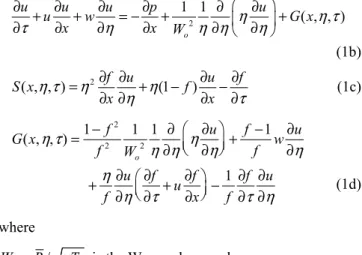
The dimensionless governing equations are (Appendix A):

( u) ( w) _{S x}_{( , , )} x η η _{η τ} η ∂ ₊∂ ₌ ∂ ∂ 1(a) 2 1 1 _{( , , )} o u _u u _w u p u _{G x} x x W η η τ τ η η η η § · ∂ ₊ ∂ ₊ ∂ _{= −}∂ ₊ ∂ ∂ ₊ ¨ ¸ ∂ ∂ ∂ ∂ ∂ © ∂ ¹ (1b) 2 ( , , ) f u (1 ) u f S x f x x η τ η η η τ ∂ ∂ ∂ ∂ = + − − ∂ ∂ ∂ ∂ (1c) 2 2 2 1 1 1 1 ( , , ) 1 o f u f u G x w f f W u f _u f f u f x f η τ η η η η η η η τ τ η § · − ∂ ∂ − ∂ = _¨ _¸+ © ¹ ∂ ∂ ∂ ∂ §∂ ∂ · ∂ ∂ + _∂ ¨_©_∂ + _∂ ¸_¹− _{∂ ∂} (1d) where 0 / o

W =R νT is the Womersley number

( , , ) ( , , ) / .

w xη τ =v xη τ − ∂ ∂f τ

As to the initial and boundary conditions: At Ĳ = 0: u x( , ,0) 1; ( ,0)_η = f x = f₀. At the wall: u x( ,1, )τ =w x( ,1, ) 0τ = . On the axis: 0 0. u η η = ∂ ₌ ∂ At x = 0: u(0, , ) 1η τ = +γ|sin 2 |; (0, ) 0.πτ p τ =

The problem is reduced to that of a rigid cylinder. The fluid-structure interaction is expressed in terms of a fluid source S(x,η, τ) in the continuity equation and an induced force G(x,η, τ) in the momentum equation.

We consider next the integral form of the continuity equation: 0( , ) 0(0, ) 0 ( , , ) d 0 (0, , ) d R x t R t U X R t R R= U R t R R

³

whose dimensionless form leads to a non-linear expression for the form factor: f(x, Ĳ):

1 ₂ 1 2 0 0 0 1 0 0 1 0 ( , , ) d (0, , ) ( , ) (0, , ) d ( , , ) d f u x f u d f x u f u x η τ η η η τ η η τ η τ η η η τ η η = =

³

(2)

f0 is the time independent form factor at x = 0.

2.2 The tube law

To close the problem, a relation linking the radius of the tube to the transmural pressure is derived. We refer to this relation as the tube law. Several propositions have been reported in the scientific literature. Kececioglu et al. (1981) obtained an expression for the local tube law through experimental observations for collapsible tubes. A more general expression is the equation of state given by Timoschenko (linear shell theory) (1951).

(4)

2 4 0 0 0 2 4 2 ( ) ( ) ( ) p m R R R R Ea a D R R P t X _R ρ ∂ − + ∂ − + − = ∂ ∂ (3) 3_/12(1 2₎

D Ea= −δ is the rigidity of the wall.

Longitudinal tension and bending are ignored, reducing the shell like behaviour of the structure to a membrane like behaviour. In the approximation of large wave length, the left hand side second term of Equation (3) is of the order of

4

( / )R λ and can be neglected. The tube law, in its non dimensional form becomes:

2 2 2 0 ( 1) m m P f A f p U β τ ρ ∂ ₊ _{− =} ₌ ∂ where 2 1. p a R A R ρ λ ρ § · § · § · =¨ _{¸¨ ¸}¨ ¸ ¨ ¸<< © ¹© ¹ © ¹ and 2 0

stiffness of the wall . dynamic pressure a E R U β ρ § · ¨ ¸ =¨ ¸= ¨ ¸ ¨ ¸ © ¹

The mass less equilibrium equation is then: (f 1) p_m.

β − = (4)

At this stage, it might be instructive to comment on this newly introduced β parameter to which we refer in this paper, as the material coefficient.

ȡU02 is twice the largest pressure drop (stagnation

pressure) within the system that is the largest load the wall would experience. Hence for ȕ > 0.5, the stiffness against area changes overcomes any transmural pressure and as a consequence, we expect the wall to contract, in which case the main assumption (axisymmetric deformation) would no longer be realistic. We shall return to this particular point in subsection 4.3. Let 0 2 0 ( ) with a , m p p p p p p U δ δ ρ − = + =

being the external pressure.

a p Back to expression (4): (f 1) pm p p. β − = = +δ 0 0

At 0,x= f = f and 0p= β(f − =1) δp that we report into the above equation to end up with a final linear expression for the tube law:

0

(f f ) p.

β − = (5)

This expression can be seen as a first order Taylor expansion of the function f = f(p) around p = 0 with

1 0 x f p β − = ∂ ₌ ∂ .

It suggests small transmural pressure p and small deformation f.

3 Numerical analysis and computational technique

The governing equations are solved numerically through finite difference technique. The non-linear terms are linearised in time through a Taylor series expansion around the previous step. The velocity profile being expected to be very steep near the wall and at the entrance, a non uniform grid is considered. The coordinates of the nodal point (i, j) in the (x, Ș) plan are given by:

( 1) 1 , ( 1) 1 1 1 and 1 1. I i x X I J j i I j J J δ ε η § _§ _{− −} _· · = ¨_¨ −_¨ _¸ ¸_¸ © ¹ © ¹ § _§ _{− −} _· · = −¨_¨ _¨ _¸ ¸_¸ ≤ ≤ + ≤ ≤ + © ¹ © ¹

X is the total length in the x direction in terms of wave lengths, I and J are the maximal number of steps in the x and Ș direction respectively, İ and į are the grid coefficients.

In order to respect the second order precision, a four nodal point discretisation for the second order derivative and a three nodal point for the first order derivative are performed. We finally use the Gaussian elimination method with partial pivoting to solve the linear algebraic equations system. Several values for I and J were tested. For J greater than 100 (ȕ < 0.5) no appreciable changes where noted. As for the grid coefficients, the values of İ = 3 and į = 0.6 in the Ș and x direction respectively are used.

Depending upon the material coefficient ȕ, two numerical algorithms are performed:

• ȕ ≥ 0.5: For x and Ĳ fixed, we guess the radial component of the velocity profile w, then use Equations (1b), (1d) and (2) to calculate the longitudinal component and the form factor f. Equations (1a) and (1c) give the new value of the radial component which is compared to the previous one. We iterate till convergence.

• ȕ < 0.5: At axial position x and time Ĳ, we guess the value of the form factor f, then use Equations (1a) and (1d) along with the tube law (Eq. 5) to calculate the velocity profile. Equation (2) gives the new value of the form factor f, which is compared to the previous one. We iterate till convergence. Meanwhile, we check both, the volume flow rate as we progress downstream and the convergence rate of the velocity field.

(5)

Fluid-structure interaction in pipe flow 357

4 Results and analysis

4.1 Preliminary results

4.1.1 Validation

The present code has been subject to two validation tests: the solution of an oscillatory rigid pipe flow and that of a contracting pipe flow are sought for. The results are validated against previously obtained results.

• Unsteady oscillatory rigid pipe flow (Appendix B). The unsteady component of the axial velocity profiles at different instants along a period, as given by the present model (Fig. 2) are compared with those given by Zhao and Cheng (1998) (Fig. 3).

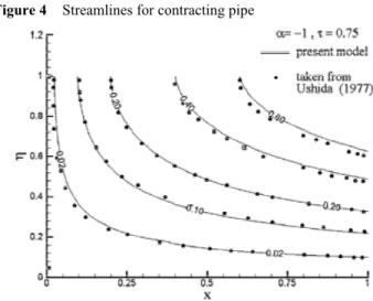
• The contracting pipe flow. We use the present model to work out the problem of the contracting tube

considered by Ushida and Aoki (1977) and to which we already referred in the introduction.

The tube being closed at the upstream end, the volume flow rate past a section x, is supplied by the fluid contained in the now diminished volume of pipe between x = 0 and x. In this particular case, Equation (2) reads:

1 0 ( ) ( , , ) . ( ) f u x d x f τ η τ η η τ ′ =

³

Figure 2 Oscillatory axial velocity components as given

by the present model

Figure 3 Oscillatory axial velocity components as given

by Zhao et al. (1998)

f is the radius of the tube which, according to the authors, should vary in time as f( )_τ = 1+_ατ in order to get an

analytical solution similar in both, time and space. _{α is a} constant that turns out to be the Womersley number as defined in the present paper.

Instantaneous streamlines as given by the two models are compared in Figure 4.

Figure 4 Streamlines for contracting pipe

We note for both tests, an excellent agreement between the results obtained by the present model and those given by previous authors.

4.1.2 Transitory/permanent regime

Figure 5 shows the behaviour of the structure over 30 periods of time. After a transitory regime that lasts about 10 periods, the system enters a permanent phase. Subsequent calculations and analysis will focus on instantaneous phenomena within this second phase (Ĳ = 30) unless otherwise specified.

Figure 5 Form factor vs. time for steady and unsteady flows

4.2 Dynamic analysis for ȕ < 0.5

In all situations, we observe at the very entrance an instantaneous throat followed by damped oscillations, the tube recovers then and inflates as we progress downstream. The section of the tube may even get large enough to cause the flow to be highly retarded and eventually to reverse at the wall.

(6)

4.2.1 Influence of the Womersley number

The form factor is a decreasing function of Wo as depicted

in Figure 6.

Figure 6 Form factor for different values of the Womersley

number at Ĳ = 30

Downstream, the pressure force tends to zero (Fig. 8), the only influencing force is G (the G induced force averaged over the corresponding section). It is a decelerating force (Fig. 7) under the action of which the flow slows down and the tube inflates to meet the classical mass conservation law.

Figure 7 Averaged induced force along the axis for different

values of Womersley number

Figure 8 Pressure force along the axis for different values

of Womersley number

At the entrance (x = 0.237) both forces, the force G (Fig. 9), and the pressure force (Fig. 8), are favourable forces.

The flow is accelerated and as a consequence an instantaneous throat is formed. It is followed by damped oscillations.

Figure 9 Induced force profiles at four different sections

Figure 10 shows that the effects of the G induced force are limited to a thin boundary layer attached to the wall and whose thickness is inversely proportional to the Womersley number. In the vicinity of the axis, this force has no effect (Uchida and Aoki, 1977) drew the same conclusion concerning the effects of the viscous forces for contracting tubes.

Figure 10 Induced G force profiles for different values

of Womersley number

4.2.2 Influence of the material coefficient ȕ

Figure 12 shows that the |G| force is an increasing function of the material coefficient. As ȕ gets larger, the flow slows down and the tube inflates as depicted in Figure 11.

(7)

Figure 12 Induced G force profile for different values of ȕ

4.2.3 Influence of the unsteady component

We shall in this subparagraph, investigate on the effects of the unsteadiness on the dynamics of the structure.

Figures 13–15 reveal that for a steady state flow (γ = 0), the tube inflates monotonously under the action of both, the induced force and the pressure force. These forces are retarding forces in the entrance region and tend to vanish as sections farther downstream are considered.

Figure 13 Form factor vs. x for different values of Ȗ

Figure 14 Steady and unsteady G force vs. x

Figure 15 Steady and unsteady pressure gradient vs. x

For_{γ ≠ 0, we observe an instantaneous contraction followed} by damped oscillations; then the tube inflates under the action of the retarding induced force and viscous force.

Figure 16 depicts the unsteady G force profile as compared to the zero Ȗ number case. It shows clearly that downstream, unsteadiness is responsible for the strong fluid-structure interaction.

Figure 16 Instantaneous profiles of G in steady and unsteady

cases

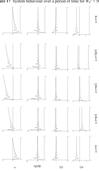
4.2.4 System behaviour over a period of time

To complete the dynamic description, Figure 17 depicts the behaviour of the structure over a period of time for ȕ = 0.4, W02 = 500, Ȗ = 0.5 and 0 ≤ x ≤ 5.

(8)

4.3 Dynamic analysis for

_{β ≥}

0.5

As expected, the model reveals that for _{β ≥ 0.5, the tube} contracts. Recall that the mathematical modelisation (Appendix A) is based on axisymmetric cylindrical Navier-Stokes equations; therefore, only inflating tubes that retain their cylindrical shape during deformation have to be considered. Contracting tubes violate this constraint and should be excluded. For this raison, this paragraph is not intended to investigate contracting tubes; it should be seen as an attempt to evidence the effects of the material coefficientβ.

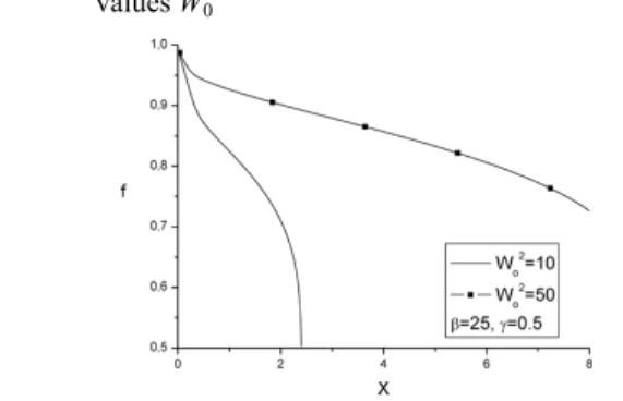
4.3.1 The form-factor

Figure 18 reveals that the deformation is a decreasing function of the Womersley number.

Figure 18 Unsteady form factors along the axis for tow different

values W0

4.3.2 Pressure force vs. averaged G induced force

Figures 19 and 20 show the pressure force and the G force along the axis.

Figure 19 Averaged induced force along the axis for ȕ > 1

Figure 20 Pressure force along the axis for ȕ > 1

We note that the accelerating pressure force is the only driving force under the action of which the tube contracts. The averaged induced force is negligible.

5 Conclusions

Motivated by biofluid mechanics problems, where the fluid-solid interaction is of primary importance, we have investigated the wall deformation of a compliant cylindrical tube conveying a viscous Newtonian fluid. The model is based on the entry length boundary layer equations associated to a linear tube law and has the particularity of setting apart terms that account for the interaction between the flow and the structure. It reveals also the non dimensional parameters that govern the dynamics of the system: These are the material coefficient which is the ratio of the stiffness of the wall to the dynamic pressure and the Womersley number which gives the dimensionless frequency of the inlet flow rate.

The Salient results are summarised bellow, then will follow a perspective for further development.

Terms that account for the fluid structure interaction are an induced force in the momentum equation and a source term in the continuity equation. The induced force affects the dynamics of the flow. It is shown for instance, that for relatively small values of the material coefficient, this force, along with the viscous force, acts to increase the section of the tube. As to the source term, it affects the form of the structure. Concerning the governing parameters, an examination of the material coefficient shows that there exists a critical value (ȕ = 0.5) above which the tube has the tendency to contract; in which case the axisymmetric approximation would no longer be physically realistic. This is corroborated by computational predictions. Concerning the Womersley number, the model shows that the structure is very sensitive to this parameter and that smaller it is, greater is the deformation.

Further development of the model will have to address the two following areas:

• extension to the full elliptic Navier-Stokes equations • extension to a non-linear tube law that accounts for

longitudinal tension.

These modifications will allow for the propagation of a finite amplitude wave area deformation along the wall. The analysis of both, the flow velocity and the longitudinal phase velocity of area variation will give deep insight into the interesting shocking phenomenon which has already been observed by previous researchers and reported in the scientific literature.

References

Demiray, H. (2002) ‘Nonlinear waves in a prestressed elastic tube filled with a layered fluid’, Int. J. Eng. Sci., Vol. 40, No. 7, pp.713–726.

(9)

Heil, M. (1997) ‘Stokes flow in collapsible tubes-computation and experiment’, Journal of Fluid Mechanics, December, Vol. 353, pp.285–312.

Heil, M. (1998) ‘Stokes flows in elastic tube-A large displacement fluid-structure interaction problem’, Int. J. for Numer. Meth. Fluids, Vol. 28, No. 2, pp.243–265.

Heil, M. and White, J.P. (2002) ‘Airway closure: surface-tension-driven non-axisymmetric instabilities of liquid-lined elastic rings’, Journal of Fluid Mechanics, July, Vol. 462, pp.79–109.

Kamm, R.D. and Shapiro, A.H. (1979) ‘Unsteady flow in a collapsible tube subjected to external pressure or body forces’, Journal of Fluid Mechanics, Vol. 95, No. 1, pp.1–78.

Kececioglu, I. et al. (1981) ‘Steady supercritical flow in collapsible tubes. Part 2 Theoretical studies’, Journal of Fluid Mechanics, August, Vol. 109, pp.391–415.

Pedrizzetti, G. (1998) ‘Fluid flow in a tube with an elastic membrane insertion’, Journal of Fluid Mechanics, November, Vol. 375, pp.39–64.

Shapiro, A.H. (1977) ‘Physiologic and medical aspects of flowin collapsible tubes’, Proc. 6th Canadian Congress on Applied Mechanics, pp.883–906.

Shapiro, A.H., Jaffrin, M.Y. and Weinberg, S.L. (1969) ‘Peristaltic pumping with long wavelengths at low Reynolds number’, Journal of Fluid Mechanics, Vol. 37, No. 4, pp.799–825.

Timoschenko, S. (1951) ‘Theorie des plaques et des coques’, Lib-polytech, Liège, Paris.

Uchida, S. and Aoki, H. (1977) ‘Unsteady flows in a semi-infinite contracting or expanding pipe’, Journal of Fluid Mechanics, Vol. 82, No. 2, pp.371–387.

Zhao, T.S. and Cheng, P. (1998) ‘Heat transfer in oscillatory flows’, Annual Review of Heat Transfer, Vol. IX, pp.1–64.

Appendix A

The Navier-Stokes axisymmetric equations in cylindrical coordinates are: 2 2 ( ) ( ) ₀ 1 1 . RU RV X R U U U P U V U t X R X V V V P U V V t X R R ν ρ ν ρ ∂ ₊∂ ₌ ∂ ∂ ∂ ₊ ∂ ₊ ∂ _{= −} ∂ _{+ ∇} ∂ ∂ ∂ ∂ ∂ ₊ ∂ ₊ ∂ _{= −} ∂ _{+ ∇} ∂ ∂ ∂ ∂ (A-1)

We introduce the following dependent and independent dimensionless variables 0 0 0 2 0 0 0 0 0 0 , , , , U T , P P. X R t U V x r u v p U T R τ T U U R ρU − = = = = = =

T0 being the period of the inlet sinusoidal velocity

(ωT0 = 2π) and P0, the inlet pressure.

In the approximation of large wave length (λ = U0T0) as

compared with the average radius R, the above equations reduce to the well-known boundary layer equations

( )ru ( )rv ₀ x r ∂ ₊∂ ₌ ∂ ∂ 2 2 2 0 1 1 u _u u _v u p u u x r x W r r r τ § · ∂ ₊ ∂ ₊ ∂ _{= −}∂ ₊ ∂ ₊∂ ¨ ¸ ∂ ∂ ∂ ∂ © ∂ ∂ ¹ 0 0

with Womersley W R number.

T ν

= ≡

The radius of the tube is written as:

0 0 0 ( , ) ( , ) . ( , ) R R r r x f x R f x R τ τ η τ = = = =

The new dimensionless independent variables are x and_η 0 and 1 0 x> ≥ ≥η 2 2 2 2 2 , 1 1 , . f x x x x f x f t f r r f r f η η η η η η τ η τ τ τ η η η η η § · ∂ _→ ∂ ₊ ∂ ∂§ ·₌ ∂ ∂ ∂ − ¨ ¸ ¨ ¸ ∂ ∂ ∂ ©∂ ¹ ∂ © ∂ ∂¹ § · ∂ _→ ∂ ₊ ∂ ∂§ ·₌ ∂ ∂ ∂ − ¨ ¸ ¨ ¸ ∂ ∂ ∂ ©∂ ¹ ∂ © ∂ ¹∂ § · § · ∂ _→ ∂ ∂§ ·₌ ∂ ∂ ∂ → ¨ ¸ ¨ ¸ ¨ ¸ ∂ ∂ ©∂ ¹ © ¹∂ ∂ © ¹∂

That we report in the above boundary layer equations, to end up with: • Continuity equation: 2 _{( ) 0.} u f u f v x x x η η η η ∂ ₋ ∂ ∂ ₊ ∂ ₌ ∂ ∂ ∂ ∂

We add on both sides of this equation the term ∂/∂x(ηu) and replace v by v = w + _{∂f/∂τ, then rearrange to get:}

( )u ( w) S( , , )x x η η η η τ ∂ ₊ ∂ ₌ ∂ ∂ (A-2) 2 ( , , ) (1 ) u f u f . S x f x x η τ η η η τ ∂ ∂ ∂ ∂ = − + − ∂ ∂ ∂ ∂ (A-3)

This is the continuity equation of a rigid tube with a source term in the referential (x,η, τ)

• Momentum equation 2 2 2 2 0 1 1 1 u u v u u f f u u x f f x p u u x W f η τ η η τ η η η ∂ ₊ ∂ ₊ ∂ ₋ ∂ §∂ ₊ ∂ · ¨ ¸ © ¹ ∂ ∂ ∂ ∂ ∂ ∂ § · ∂ ∂ ∂ = − + _¨ + _¸ ∂ © ∂ ∂ ¹

(10)

Let v = w + ∂f/∂τ, add on both sides of this equation 2 2 2 0 1 1 u u u w W η η η η   ∂ ₊ ∂ ₊ ∂   ∂  ∂ ∂ 

and rearrange, to end up with:

2 2 2 0 1 1 ( , , ) u u u p u u u w G x x x W η τ τ η η η η   ∂ ₊ ∂ ₊ ∂ _{= −}∂ ₊ ∂ ₊∂ ₊   ∂ ∂ ∂ ∂  ∂ ∂  (A-4)

(

)

22 2 0 1 1 1 1 , , 1 . f u f u G x w f f W u f f f u u f x f η τ _{η η} η _η _η η η τ τ η   − ∂ ∂ − ∂ = _ _+   ∂ ∂ ∂ ∂ ∂ ∂  ∂ ∂ + _∂ __∂ + _∂ _− _{∂ ∂} (A-5)

This is the momentum equation of a flowing fluid in a rigid tube with an additional force G.

The dimensionless boundary and initial conditions are those given in the text.

Appendix B

It is well known that for the oscillatory pipe flow, the maximum axial velocity occurs near the wall and not at the centerline of the pipe as for the steady case. It is the ‘annular effect’.

Shown in Figure 3, are the velocity profiles, Zhao and Chang (1998) obtained by sweeping one period of time. The present model, associated with the superposition principle (for reasons given below), evidences the same phenomenon.

The parabolic aspect of the momentum equation implies that the numerical scheme is based on the marching in x technique. The flow at axial position x, determines that at axial position x + dx. Information progresses in the direction of increasing x. In an oscillatory flow, there is a phase of negative flow rate during which the velocity reverses. Dynamic information is then convected by the fluid in the direction of decreasing x, that is in the opposite direction of the numerical scheme. This incompatibility between the numerical and the physical aspects leads to severe numerical instabilities. During tests which we carried out, we noted indeed that when the inlet velocity became negative or when the flow reversed at the wall (excessive growth of the tube’s section), the numerical scheme diverged.

In order to circumvent this difficulty, we used the well known method of superposition which we shall describe succinctly hereafter:

• Solve for the instantaneous velocity profiles u1(x, η, τ)

when the flow is pulsating; i.e., with an inlet velocity ui(η, τ) = 1 + γ sin (ωτ) with 0 < γ < 1 (inlet flow

rate > 0 ∀τ).

• Solve for the velocity profiles u2(x, η) when the flow is

stationary; i.e., with an inlet velocity ui(η) = 1.

• Provided the governing equation is linear,

u(x, γ, τ) = u1(x, γ, τ) – u2(x, γ) (would be the velocity profiles of a reciprocating flow, i.e., with an inlet velocity ui(τ) = γ sin (ωτ).

The equation we are dealing with is not linear owing to the inertia term. However, as we approach the fully developed region downstream, the inertia term in the momentum equation gets smaller (to become zero in the fully developed region) and the equation can be considered as linear. The above superposition procedure becomes fully justified.

We used this approach with 2

0 10, 0.5, 30

W = _γ = x=

and obtained the results depicted in Figure 2 which are in excellent agreement with those obtained by Zhao and Chang (1998) (Fig. 3) that used the full elliptic Navier-Stokes equations.

The discrepancy in the numerical values is owing to the amplitude γ which is different. (γ = 0.5 in the present case against 1 for Zhao and Chang (1998)).

Nomenclature

a Thickness of the wall E Young modulus G Induced force

P, p Dimensional and dimensionless pressure pm Transmural pressure (internal-external) R Dimensional radial coordinate R0 Radius of the tube

R Average radius of the tube S Fluid source

t Time

T0 Period of the inlet flow rate

U, u Dimensional and dimensionless axial velocity U0 Inlet dimensional velocity

V, v Dimensional and dimensionless radial velocity Wo Womersley number

X, x Dimensional and dimensionless axial coordinate Greek symbols

β Material coefficient

γ Amplitude of the oscillatory component of the inlet flow

δ Poisson modulus