Ab initio modeling of complex aqueous and gaseous systems containing nitrogen

Ab Initio Modeling of Complex Aqueous and Gaseous

Systems Containing Nitrogen

by

Robert

Wilson

Ashcraft

B.S. in Chemical Engineering

B.A. in Chemistry

North Carolina State University (2003)

MASSACHUSETTS INSTr E

OF TECHNOLOGY

SEP

10

₂₀₀₈

LIBRARIES

M.S. in Chemical Engineering Practice

Massachusetts Institute of Technology (2005)

Submitted to the Department of Chemical Engineering in partial fulfillment of the requirements for the degree of

DOCTORATE OF PHILOSOPHY IN CHEMICAL ENGINEERING at the

MASSACHUSETTS INSTITUTE OF TECHNOLOGY September 2008

© 2008 Massachusetts Institute of Technology. All rights reserved.

Signature of Author

Department of Chemical Engineering August 27, 2008

Certified by:

CI

Accepted by:

William H. Green Professor of Chemical Engineering Thesis Supervisor

William M. Deen Professor of Chemical Engineering Chairman, Committee for Graduate Students

Ab Initio Modeling of Complex Aqueous and Gaseous

Systems Containing Nitrogen

by

Robert

Wilson

Ashcraft

Submitted to the Department of Chemical Engineering on September 27, 2008 in partial fulfillment of the requirements for the degree of Doctor of Philosophy in Chemical Engineering

Abstract

Nitrogen chemistry is ubiquitous in everyday life, from biological processes at ambient con-ditions to atmospheric chemistry at low pressures and temperatures to high-temperature combustion. Understanding the chemical behavior of nitrogen-containing species under a variety of conditions and in multiple phases is critical to accurately modeling system behav-ior. The further ability to model system behavior based solely on a first principles approach would be a boon to researchers attempting to design and understand technologies utilizing complex systems. This work attempts to further these abilities for both solution-phase and gas-phase predictions from ab initio calculations,

An overview of solvation thermodynamics is given that relates computational chemistry to phenomenological thermodynamics for common equilibrium expressions. Special attention is paid to fully understanding the role of activity coefficients, standard states, and reference states and how these affect the subsequent expressions.

A procedure is outlined for estimating the thermochemical properties of small molecules in aqueous solution based on computational chemistry calculations utilizing continuum solva-tion models. The partisolva-tioning of the entropic and enthalpic contribusolva-tions is of the utmost importance if one is to accurately estimate the enthalpy of formation and entropy in solu-tion. Procedures for rate coefficient estimation via solution-phase transition state theory, simple electron transfer theory, and dissociative isomerizations within a solvent cage are also discussed. The oxidation of hydroxylamine in aqueous nitric acid was chosen as a test system. A detailed chemical mechanism was constructed and thermochemical and rate parameters from computational chemistry calculations were used to model the behavior of the system. Using current continuum solvation models, it does not appear possible to build reliable predictive models of complex aqueous systems, particular those with a high ionic strength. However, the present semi-quantitative models may be helpful in focusing atten-tion on the key unknowns.

Group additivity values were estimated for more than 50 new functional groups containing nitrogen based on high-level computational chemistry estimates of the thermochemical

pa-rameters of 105 non-cyclic C/H/N/O species. The thermochemical and kinetics databases of the group's Reaction Mechanism Generator software were restructured to be more ex-tensible and to explicitly include nitrogen chemistry. This allows new chemistry to be added to the software more easily and will allow predictions for gas-phase nitrogen-containing systems in the very near future.

Acknowledgements

First and foremost I would like to thank my wife. She has gone to great lengths and en-dured much stress and anxiety to be in Boston, all so that I could realize my ambition to go to MIT. Without you, this would have been a lonelier, less gratifying, and much more tor-tuous (yeah, that's for you) path.

Next, I thank my entire family for there unending support in every way; always encouraging me to strive for more, there when needed, and providing welcome diversions along the way. Same to the Burris's, you have also all been great; thank you!

Bill, you have been and excellent thesis advisor, career counselor, and person over the last four and half years. You have supported me in going to practice school and Singapore; both of which were great experiences, and I am glad you realized that and encouraged me to go. All of your students should feel fortunate to be under you care and guidance.

Professors Trout and Tidor, thank you both for your guidance, helpful discussions, and cri-tiques throughout the years. You both made my research more impactful and relevant. The entire Green group, past and present; you have been great to work with, have fun with, and procrastinate with. I could not have asked for a better group of people with which to spend five years of my life.

Sumathy, you were an essential mentor when starting this work and made my life much easier through your guidance and expertise. You were always there with answers and en-couragement, be it technical or personal, despite any personal or professional challenges you may have been going through. It was much appreciated.

MIT friends.., you all made life much more fun, and you know who you are.

Athletes: I wanted to thank all the people I had the pleasure of playing intramurals or rec-reational sports with. These activities definitely made my life significantly more enjoyable, and it would not have been possible or nearly as fun without the dedicated and talented group of people we have in our department. Keep representing our department proudly

(and with good sportsmanship).

Lastly, I would like to thank MIT for creating an institution that treats its student well, en-sures we have access to the best people and tools, and provides such a wide breath of po-tential experiences.

Table of Contents

I

Intro d uctio n ... I I

2 Solvation Thermochemistry Fundamentals ... 15

2 .1 In t ro d u c tio n ... ... ... ... ... . ... 15

2.2 Derivation of a Condensed-Phase Equilibrium Expression ... 19

2 ,2 . I D e riv atio n ... ... ... ... .... ... ... ... ... 2 0 2.2.2 Understanding the Use of Standard and Reference States ... 25

2 .3 Practical Equilibrium Ex p ressio ns ... ... 29

2.4 Solution-phase T ransition State T heory ... ... 3 1 2.5 Sum m ary ... ... 36

2 .6 A p p e n d ic e s ... ... ... ... 3 7 2.6. I Nomenclature ... ... .. ... 37

3 Solution-Phase Thermochemistry from Computational Chemistry ... 39

3. 1 Introduction ... ... .... ... 39

3.2 Theoretical Basis - Solvation Therm ochem istry... ... 4 I 3 .2 .1 V a p o r-L iq u id E q u ilib riu m ... 4 4 3.2.2 Chemical Reaction Equilibria ... .. ... 46

3.2.3 AGo and AG* from Computational Chemistry... ... 47

3.3 C om putational M ethodology ... ... 50

3.3. I G as-Phase Therm ochem istry . ... 50

3.3.2 Solution-Phase T herm ochem istry ... ... 5 I 3.3.2. 1 Solution-Phase and Solvation Entropy ... ... 59

3.3.2.2 Solution-Phase Enthalpy of Formation ... 62

3.3.2.3 N on-Ideal Effects... . ... ... ... 63

3.4 Results and D iscussion ... 64

3.4. 1 G as-Phase Estim ates ... ... 64

3.4 .2 So lutio n-Phase Estim ates... ... ... .... ... 65

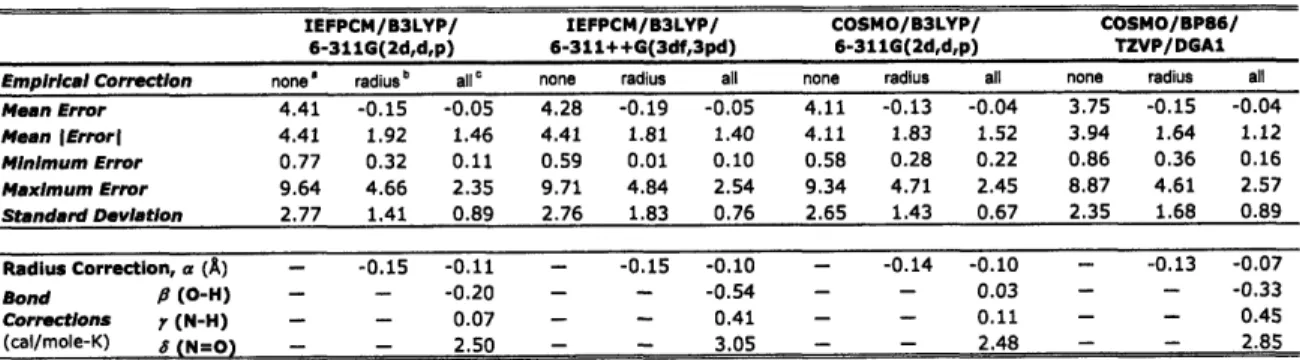
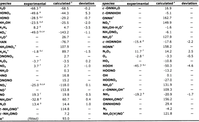
3 .4 .2 .1 E ntro p y R e su lts ... ... ... 6 6 3.4.2.2 Enthalpy of Formation Results ... 69

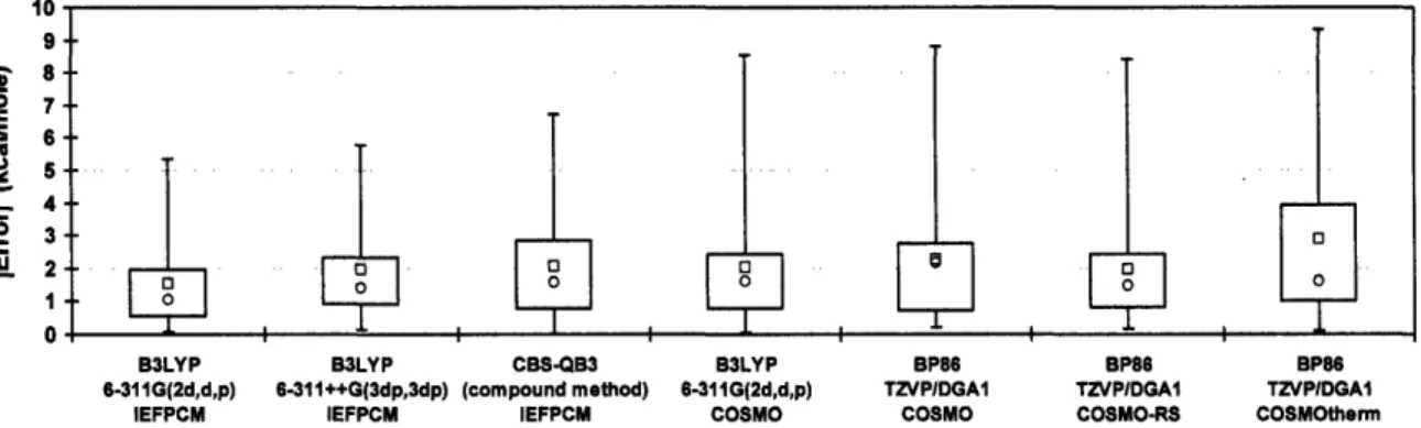
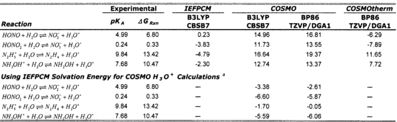
3.4.3 Comparison with Experimental Aqueous Equilibrium Data... 72

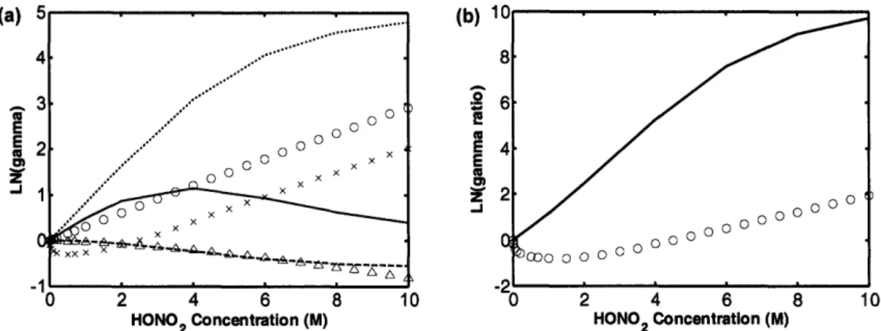
3.4.4 A ctivity C oefficient Estim ates ... ... 73

3 .5 C o n c lu s io n s ... ... 7 6 3 .6 A p p e n d ic e s ... . . ... ... ... ... 7 8 3.6. I G as-Phase Enthalpy Estim ates ... ... 78

3.6.2 Solution-Phase BAC Bond Assignments ... 79

3.6.3 Infinite-Dilution Activity Coefficients via COSMOtherm... 80

3.6.4 Bond Assignments in the Solvent-Ordering Entropy ... 81

3.6.5 Structures of M olecules in Solution ... ... 82

4 Solution-Phase Kinetics and M odeling ... ... 91

4.1 Introduction .... ... 91

4.2 Com putation M ethodology ... ... ... .. 93

4 .2. I T he rm o che m istry Estim atio n ... ... ... 9 3 4.2.2 Rate Coefficient Estim ation ... ... 94

4.2.2. 1 D iffusion-lim ited ... 95

4 .2 .2 .2 T ransitio n State T heo ry ... ... 9 6 4.2.2.3 Electron Transfer Reactions ... ... ... 99

4.2.2.4 Reactions in Solvent Cages ... .. .. ... .... ... .... 100

4.3 Mechanism Developm ent ... 104

4.4 Results and Discussion ... 06

4.4. I Rate C oefficient Estim ates ... ... I 06 4.4. I .I Transition State Theory ... ... 06

4.4.1.2 Electron Transfer ... ... ... 1 12 4,4.1.3 Solvent Cage Reactions ... ... 1 15 4.4.2 M odeling Results and D iscussion... ... ... 1 19 4.4.2. I Thermochemistry and Rate Coefficient Corrections... 20

4.4.2.2 Initial M odel... ... 121

4.4.2.3 Sensitivity Analysis ... ... ... ... 26

4.4.2.4 Final Model ... ... 129

4 .5 C o n c lu s io n ... ... ... ... . .. ... 3 3 4.6 A ppendices .. ... ... ... ... ... ... ... 135

4.6. I Effect of Non-Electrostatic Solvation on the Reaction Barrier... 135

4.6.2 Additional DISC Reaction Information ... ... ... 137

4.6.3 Molecular Radii ... ... 138

4.6.4 D iffusion-lim ited rate coefficients calculations... ... 139

4.6.5 Electron-transfer rate coefficient calculations... 40

4.6.6 Activity coefficient estimates for major species ... 43

4.6.7 B3LYP and MP2 reaction barrier comparison ... 145

5 Gas-Phase Group Additivity Values for C/H/N/O Species ... 147

5. 1 Introductio n ... . . ... ... 47

5.2 M ethodology ... ... .... ... 147

5.3 Results and D iscussion ... ... ... ... .... ... 50

5.4 Conclusion ... ... ... 60

5.5 Appendices ... 62

5.5. I1 Table of Equivalent Molecular Names ... 62

5.5.2 Test Set M olecule Construction and Group Values... 63

5.5.3 Two-dimensional structural schematics of all molecules studied ... 164

5.5.4 Two-dimensional structural schematics of all groups derived ... 69

5.5.5 G roup A ssignm ents for M olecules ... 173

5.5.6 Cartesian Geometries for Molecules ... ... ... 173

6 Nitrogen Chemistry in Automatic Reaction Mechanism Generation ... 175

6. I Reaction M echanism G enerator... ... ... ... 175

6. 1. I A lgorithm ... . .... 176

6. 1 .2 T he rm o chem ical D atabase ... ... 177

6. I1.3 Kinetics and Reaction Fam ilies... 178

6.2 Challenges of Adding New Chemistry ... ... 178

6.3 Thermochemistry Database Restructuring... ... 80

6.3. I1 Revised Database Functional Group Atom s ... ... .... 182

6.3.2 Revised Tree Structure ... ... 86

6.3.2. I Revised M ain Therm ochem istry Tree... ... ... 87

6.3.2.2 Revised Radical Increment Tree ... ... 192

6.3.2.3 New Group Centric and Group Adjacent Trees ... 93

6.3.2.4 Potential Alternative to Group Centric/Adjacent Trees... 20 I1 6.3.3 R evised Library Entries... ... ... 22 1 6.4 Reaction Fam ily Restructuring ... ... 221

6,4, 1 Tree Structure Changes and the Addition of Nitrogen ... 222

6.4.2 Merging of Similar Reaction Families ... 224

6.4.2. 1 Radical Recom bination Fam ilies ... ... ... 225

6.4.2.2 Radical Disproportionation via H-transfer Families... 225

6.4.2.3 2+ 2 C ycloaddition ... ... 226

6.5 Necessary Modifications and Recommended Improvements ... 226

6.5. I N ecessary M odifications ... ... ... ... ... 227

6.5., 1 I Flexible Functional Group Atoms ... 227

6.5. I .2 Resonance Structure G eneration ... ... 232

6.5.1.3 Reaction Fam ilies w ith N 3/N 5 Conversions ... 234

6.5,1.4 N eighboring Radical Bond Form ation ... .... ... 235

6.5.2 Suggested Im provem ents ... ... ... ... ... 236

6.5,2. 1 Referring Nodes without Data to Those with Data... 236

6.5.2.2 Multiple Primary Thermochemistry and Kinetics Databases... 237

6.5.2.3 Reporting of Group Values Used in Estimates ... 237

6.5.2.4 Warnings for Use of Dissimilar Groups ... 239

6.5.2.5 Warnings for Small Molecules via Group Additivity... 240

6 .6 A p p e n d ic es ... .... .... ... ... ... ... 2 4 1 6.6.1 Listing of Functional Group Atoms in Revised Database ... 24 I1 6.6.2 Group Adjacent Tree and Library ... ... 249

6.6.2. I G ro up A djacent T ree ... . . ... ... ... 249

6 .6.2.2 G ro u p A djace nt Lib rary ... 2 5 1 6,6.3 Radical Increments for Nitrogen-containing Groups ... 252

7 Sum m ary ... 255

8 G eneral A ppendices ... 259

8.1 Using the "tst2c I " Rate and Thermochemistry Code ... 259

8. I .I G eneral Pro cedures ... . . . ... .. ... 259

8.1 .2 Exam ple of "tst2c I " U sage ... ... .... .... ... ... ... 267

8.1.3 Using "calc_rho" to determine rotor energy levels ... 273

8.2 Solvation Energies from Gaussian03 and COSMO-RS and Their Relation to E q u ilib riu m D ata ... ... ... 2 7 4 8.2. I Background Inform ation ... ... ... ... 274

8.2.2 Interpreting the Results from Gaussian03 PCM Calculations... 277

8.2.3 Interpreting the Results from COSMOtherm Calculations ... 279

8.2.4 Using the Com putational Chem istry Data ... 284

8.2.5 _{Henry's Law Analysis - Computational and Experimental Data... 286}

8.2.6 C hanging Standard States to PC P... ... ... ... ... 293

I

Introduction

The construction of complex chemical-physical models in the absence of experimental data

is a continuing goal of the scientific and engineering community. If accurate enough, these

predictive models could be used to design new systems, avoiding much of the expensive Edisonian experimentation that slows innovation. Even when the predictive models are not accurate enough for design, they often allow for identification of key reaction paths and to help guide experimental studies. In many cases, it is the inability to predict thermochemical data and rate coefficients accurately that has limited the success of such attempts. Ideally, one would like to build an entire mechanism based solely on ab initio calculations capable of making reliable predictions.

In the gas phase, this is becoming possible for some systems if one makes use of all avail-able tools, including those that use microcanonical rate constants over many energy levels to accurately predict rate coefficients as a function of temperature and pressure. There is a large community devoted to developing these methods, and much has been published demonstrating their accuracy and applicability. In recent years, a number of highly-complex and very successful chemical kinetic models have been constructed for gas-phase C/H/N/O

systems."2 _{For example, predictive kinetic models based on quantum chemical calculations}

identified the true pathway by which CH + N2 leads to NOx formation,3_{' the pathway to}

NOx formation through NNH in low-T flames,5_'6 _{and the autocatalytic pathway in methane}

pyrolysis.7 _{However, the detailed behavior of complex, gas-phase hydrocarbon systems}

involving bound nitrogen is still not known precisely, and predicting condensed-phase chemical kinetics has proven much more difficult due to the lack of accurate, computation-ally-efficient quantum solvation models. The goal of this work was to build upon previous advances in the kinetics, thermodynamics, and computational chemistry communities to extend our ability to model the chemistry of nitrogen-containing systems in both the gas and solution phases. The gas-phase and solution-phase systems were approached in differ-ent manners, in an attempt to provide valuable contributions to each.

The solution-phase work required a multi-step approach due to the relative lack of infor-mation available on how to model complex systems from ab initio calculations. The first phase of research was focused on understanding the fundamentals of solvation

thermo-chemistry and the expressions necessary to build kinetic models. The relationship between the chemical potential, activity coefficients, reference states, and standard states was investi-gated, particularly as it relates to the computational chemistry approach taken in this work. Chapter 2 is devoted to the explanation of this topic, delving into how activity coefficients change with reference and standard states, the derivation of various equilibrium expressions and constants, and how transition state theory is applied in solution-phase systems.

The next part of the solution-phase work focused on determining how to calculate the thermochemical properties of species in aqueous solution using computation chemistry techniques. Most previous work in this area has been aimed at obtaining accurate solvation free energies, as this is often the most important parameter when determining if a process is thermodynamically favorable. However, for a kinetics point of view, it is important to have enthalpy and entropy separately, both to better understand reactivity and to better capture the temperature dependence of a rate coefficient. The accurate computation of the enthalpy and entropy separately also allows for direct comparison to experimental data of those types, which is essential to understanding the accuracy of the methods. In this vein, we developed a procedure to take computational chemistry output from a continuum solvation model calculation and use it to estimate the enthalpy and entropy in solution at standard temperature and pressure. The method is slightly parameterized for the small

molecule C/H/N/O species investigated, but could be easily extended to other systems. The oxidation of hydroxylamine in aqueous nitric acid was chosen as a test system with which to develop this methodology. Chapter 3 is devoted to explaining the method, pro-viding estimated enthalpy and entropy data, and comparing the estimates with known

ex-perimental data.

Following development of the thermochemistry estimation procedure, the dynamics of the chemical system was addressed. Estimating the rate coefficients of reaction in solution was challenging in several regards: (I) there are interesting reaction types and transition state structures that occur in aqueous solution that would be unfavorable in the gas phase; (2) uncertainties generally lead to significant errors; (3) non-ideal effects are often important and difficult to characterize; and (4) there have been few, if any, previous attempts to model a complex chemical system in the manner attempted here. The rate coefficients for

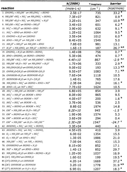
over 90 reactions associated with the oxidation of hydroxylamine were estimated based physical arguments, transition state theory, electron transfer theory, or a method for esti-mating the dissociative isomerization rate within a solvent cage (developed in this work).

Even in these static continuum calculations, the role of explicit solvent molecules can be important, both in terms of calculating an "accurate" rate constant and in simply allowing a transition state to be found. We attempt to examine some of the important roles solvent molecules may play in aqueous reactions. The effect of the so-called non-electrostatic sol-vation energy on rate coefficients is also examined, particularly as it relates to the cavitation free energy and entropy and their changes during a reaction. These topics are discussed in detail in Chapter 4.

The final part of the solution-phase work involved modeling the test system in an attempt to reproduce experimental data and to identify the most important reactions and species. The modeling efforts are also discussed in Chapter 4. The aforementioned rate and ther-mochemical data were used to construct a detailed chemical mechanism, which was simu-lated in a constant volume batch reactor. The product yields as a function of initial hydro-xylamine concentration, initial nitrous acid concentration, and initial nitric acid concentration were simulated and compared with experimental data. The time-scale of the overall reac-tion was also investigated. Sensitivity and flux analysis allowed us to propose several spe-cies and reactions that may be important in fully understanding the evolution of the system. Uncertainties in the model parameters were large, and several adjustments were needed to reach reasonable agreement with the experimental yield and ignition time data. Although the uncertainties prevent a firm determination of the most dominant pathway, we believe this type of approach can yield useful information that can guide experimental efforts and provide insight into potentially important species and reactions.

The gas-phase work related to nitrogen chemistry had an entirely different focus because estimation methodologies and modeling techniques are already well-established. This work was aimed at increasing the base of nitrogen data available to researchers and to advance the automatic Reaction Mechanism Generator (RMG) created by various members of the Green Research Group. RMG is a database-driven tool that constructs detailed chemical mechanisms based on a combinatorial approach to searching for possible reactions. It

de-termines the most important reactions based on the overall flux of the reaction relative to the system's characteristic flux. This approach requires the ability to estimate the thermo-chemistry of an arbitrary species and the rate coefficient of any included reaction type; this

is accomplished using a thermochemical and kinetic parameter database. The initial data-bases were constructed to allow for estimates for C/H/O species, with little regard for other elements, necessitating a major change in the database structure.

The initial thrust of the gas-phase work, described in Chapter 5, involved deriving group additivity values for use in thermochemical parameter estimation. Approximately 50 group

values were derived from high-level computational chemistry calculations of 105 non-cyclic

C/H/O/N molecules. Enthalpy values were fit to CBS-QB3 level enthalpies of formation, and the entropy and heat capacity values were fit to statistical mechanical estimates that accounted for hindered internal rotations. Uncertainties in the group values were esti-mated using a traditional confidence interval approach combined with Monte Carlo sam-pling to attempt to capture the effect of uncertainty in the molecular thermochemistry es-timates. These were then added to the RMG thermochemical database, which should help to extend its applicability beyond the native C/H/O chemistry subset.

However, the data could not be entered into the database initially because the original RMG database was not designed to be easily extensible to other types of chemistry. I first had to reconstruct the thermochemistry database from the ground up, paying special atten-tion to future extensibility of the database. The structured hierarchy focused first on the central atom, whether it was bonded to C/H atoms or heteroatoms, what types of bonds the central atom makes with its neighbors, and so on. In addition to the thermochemistry, the kinetics database also needed retooling, though not as drastically. All of the reaction families were modified to allow nitrogen reactions when appropriate, as well as other small changes to streamline the tree structure. Data from the literature was then used to popu-late the nitrogen portion of the kinetics tree. Despite the availability of some nitrogen-containing species and reaction data, the databases as they relate to nitrogen are still very sparsely populated, and a concerted effort to add more data should be made to improve reliability. A detailed discussion of these topics is given in Chapter 6.

2

Solvation Thermochemistry Fundamentals

2.1

Introduction

The topic of condensed-phase phenomenological thermodynamics is covered in some

de-tail in a number of chemical engineering and physical chemistry texts, as well as other

sources.8_{-12 However, finding a complete description of practical relationships in which all}

of the many assumptions are explicitly described remains an elusive task. The unfortunate reality is that many scientists and engineers are left with the option of using a relationship that they do not fully understand or devoting a significant amount of time to understand the topic "completely." We fear that the former is the more common course of action. This piece aims to provide a more thorough understanding of the concepts for knowledge-able non-experts who are not aware of or do not immediately comprehend many of the implicit assumptions made in modem texts. It will also serve as a backdrop to the work presented later in chapters 3 and 4, and we believe that fully understanding the fundamen-tals of solvation is a prerequisite to any modeling activities. It is hoped that readers will come away with an appreciation for how the choice of standard states and reference be-haviors affect the validity of common assumptions and the interpretation of activity coeffi-cients. It is assumed that the reader has knowledge of the concepts of chemical potential, fugacity, and their general uses, as is available in many chemical engineering thermodynam-ics texts. General vapor-liquid equilibrium (VLE), Henry's Law, vapor pressure, condensed-phase reaction equilibria, and condensed-condensed-phase transition state theory (TST) will be dis-cussed. Although this work is applicable to ionic systems, we will focus on standard and

reference states that are most applicable to non-ionic solutes and solvents. Information

about specific issues related to ionic systems and how to reconcile them can be found in

the literature and textbooks. 3-'5

Standard and reference states, and how these affect the definition of the activity coefficient, are often the crux of confusion when dealing with solution-phase thermodynamics. Let it be clear that the choice of the reference behavior is completely arbitrary and often repre-sents an unphysical situation. Standard states are also arbitrary, but most often represent a condition of the system where data is available, or at least an idealized incarnation of such a condition. They are simply starting points from which the behavior of a real state of the

system can be described. The states may also be defined differently for each molecule in a system of interest, and doing so may be quite useful. These points will be illustrated below in some detail.

Often, experimental data in aqueous solution are reported at a standard state of I M or

I molal. In computational chemistry calculations, energies are determined in the infinite-dilution limit and often extrapolated to a standard state of 0.041 M using gas-phase parti-tion funcparti-tion expressions. If the molecules in the system are completely miscible, a pure component standard state is sometimes used. There are two common reference behav-iors for non-ionic aqueous systems: the Henry's Law reference that describes the limiting behavior as the mole fraction of the species approaches zero, and ideal solution behavior

(known as Raoult's Law or the Lewis-Randall reference). These are just a few common examples of standard states and reference behaviors that may be used, and the proper choice will depend upon the system and availability of data. The numerical value of some thermochemical quantities will differ depending on this choice, with many possibilities for

confusion.

The treatment of solvent effects on the thermochemistry and kinetics of systems in con-densed phases has been studied theoretically and empirically in a number of fields. Often ambiguities present in the underlying assumptions and confusion with regard to standard and reference states can cause difficulty when attempting to use data or equations cor-rectly. An example of where confusion arises could be in the typical concentration-based equilibrium constant (Kc), which is a physical property of the system. However, the free energy change of reaction that it is related to in phenomenological thermodynamics is the standard state change (AGO,), since the true free energy change at equilibrium must be zero. This means that there are an infinite number of AG,, values because the standard state may be chosen arbitrarily. The same problem is seen for gas-phase systems, but it is less problematic because there is universal agreement on the conventional standard state: an ideal gas at 298 K and one atmosphere or bar of pressure. One also must be careful to use the same "zero" for the energies of the species. In solution-phase thermochemistry,

along with the typical assumption that elemental species have a zero enthalpy of formation. It is also possible to estimate an absolute enthalpy of formation for aqueous H', which would constitute a completely different "zero" of the system. This paper is written under the assumption that a consistent "zero" of energy has been used throughout. This is unre-lated to the reference used to define the activity coefficient for a species, but is important nonetheless.

The fugacity is a convenient way to express the non-ideality of a system; for ideal solutions a species' fugacity is a linear function of its mole fraction. The fugacity is defined in terms of the chemical potential of the molecule and is based upon an arbitrary reference condition (the reference can be the standard state or an arbitrary reference state) as shown in equa-tion (2-1). It is important to understand a few key properties of the fugacity. Generally, the fugacity of a molecule is dependent on the temperature, pressure, and composition of the system. For simplicity, the temperature and pressure dependences will not be ad-dressed, but it is important to understand they are present. If two systems are in

equilib-rium, then the fugacities of each species must be equal in both systems, as is the case with chemical potentials. For a vapor-liquid equilibrium situation, the fugacity (and chemical po-tential) of each species will be the same in the liquid phase and the gas phase. In a simple, pure system, this means that the fugacity of the pure liquid is equivalent to the fugacity of the pure vapor. If the vapor phase behaves ideally, then the fugacity in both phases is the vapor pressure of the pure liquid. For a multicomponent equilibrium with an ideal vapor phase, the fugacity of each species in the condensed phase is the partial vapor pressure of that component. The fugacity and vapor pressure will change depending on the interac-tions in the condensed phase, which are the source of non-ideal behavior and are de-scribed by the activity coefficients. All quantities discussed in this paper are intensive prop-erties, independent of the size/mass of the system.

f

.exp,

_RT

-

(2-1)

Equation (2- 1) illustrates a common way to define the relationship between the chemical potential and the fugacity at two arbitrarily chosen states, the actual state (#) and standard

state (o) in this case. Here,

1f7

and p7 are the fugacity and chemical potential at a chosen standard state of the system, and • and pi are the fugacity and chemical potential at the actual state of the system. If the chosen standard state exists, then

1

would be the stan-dard state vapor pressure, if the gas phase behaves ideally. If a hypothetical stanstan-dard state is chosen, then

1

has no direct physical interpretation, but can be thought of as the vapor pressure of the hypothetical state. The standard state chemical potential is defined by the zeros of energy chosen for the system, e.g. elemental forms have a chemical potential of zero. You will also notice later on that we only see a ratio of fugacities and/or differences in chemical potentials in pertinent equations. So the choice of standard state, and the nu-merical values used for

1

and p,, will not affect our predictions as long as the same standard states and numerical values are used consistently throughout.

In all equations, an "o" superscript will be used to signify the chosen standard state, a "+"

for the chosen reference state/behavior, a "#" for the actual state of the mixture, an "oo"

for the dilute-limit reference behavior, and a "pure" for the pure i reference behavior. A circumflex or "hat" on the fugacity indicates that it is a fugacity in a mixture, where as an f

without a hat indicates a pure-component fugacity. For example, p7 is the chemical po-tential at the actual state of the mixture, and p7 is the chemical popo-tential at the standard state condition. The symbol xi will be used for condensed-phase mole fractions, and y; will used for gas-phase mole fractions (or pi for the partial pressure).

The "state" and "behavior" terminologies will be used here regarding the activity coefficient reference, and it is important to understand the difference. Reference behavior describes the variations of fugacity under certain assumptions over the entire mole fraction range, fJ (x,), which is typically linear as with Henry's Law or ideal solution behavior. A refer-ence state is a single point evaluated at a specific mole fraction along the referrefer-ence behav-ior line, e.g.

J

(x, = x#). Although the reference behavior may be defined in an arbitrary manner, a simple and useful convention is to define the reference behavior for a molecule only in terms of its mole fraction: J (x ) = a + b. xi. In general, o is taken to be zero

be-cause the fugacity approaches zero with the mole fraction, and b is taken to be a fugacity value at a mole fraction of one. The reference behavior for species i is assumed to only be a function of xi for simplicity, and because assuming a more complicated dependence on

other species would implicitly include non-idealities in the reference. If b = f""", then this

amounts to assuming ideal solution behavior for the reference. If one wanted to use a

Henry's Law reference, then there is an additional complication that f, = F

(x)

because

the behavior as xi -- 0 depends on the interactions of species i with the solvent and all

other solutes. However, in this paper we will make the common simplifying assumption that our Henry's Law reference will always be for the molecule in pure water, i.e.

f+ = xiJ~ " where f" is a constant chosen so that f+ accurately approximates the actual

fugacity,

f',

as x, -- O. The key point to understand is the reference behavior is chosen

so that it only depends on the molecule of interest, whereas both the standard state and actual state behaviors can be complicated functions of the mixture composition. As will be shown later, the activity coefficient is left to capture these complex dependencies.

2.2

Derivation of a Condensed-Phase Equilibrium Expression

A non-equimolar, solution-phase equilibrium constant will be derived to illustrate the im-portant assumptions needed to arrive at equations most often given in the literature. The derivation is based on the concept of fugacity as a means to relate the chemical potential in the actual state to some arbitrary reference behavior. The two reference behaviors

dis-cussed earlier are illustrated by dashed lines in Figure 2- I, which was adapted from the 3rd

edition of Thermodynamics and Its Applications by Tester and Modell.,5 _{Henry's Law is the}

extrapolation of the fugacity slope at low concentrations to the hypothetical fugacity at

xi = I (Jf"), and ideal solution behavior is a straight line connecting zero and the pure

I

f^#

Uo

u-ure

I IUII I aI LClIUI I ,iJ

Figure 2-I: Graphical representation of two fugacity reference behaviors and the corresponding activity

coef-ficients needed to correct to actual behavior. 2.2.1 Derivation

The fugacity embodies the non-ideal nature of a mixture at a given condition and serves to relate the chemical potentials at two different conditions. As shown in equation (2-2), knowing the fugacity of a species under two conditions will yield the chemical potential dif-ference. Equation (2-2) also shows how the fugacity and the activity are related, though the activity will not be explicitly used here: in our opinion it is more pedagogical to work with fugacity instead. Equation (2-3) gives the chemical potential difference between the actual state and a standard state.

Ajliq

= uiq + RT

In

= +liq +RT

In

(a)

(2-2)

Aliq oiq + RT

In(Ii

= ,q + RT In

ai

(2-3)

In these expressions, /ui# is the chemical potential in the actual state, A,'2iq is the standard

state chemical potential, fg is the fugacity in the actual state, and fo is the fugacity in the

standard state. Since the goal is to derive an equilibrium relationship for the example

reac-tion A N B + C, one must realize that the actual state chemical potentials of A and B + C

are equal at equilibrium. Writing equation (2-3) for each species and setting the chemical

potentials equal yields equation (2-4), dropping the explicit condensed-phase notation. A simple rearrangement of the terms allows one to extract the well-known activity-based equilibrium constant, KA, which is defined in terms of the standard state chemical potential difference or the standard state Gibbs free energy change of reaction, AG',, as shown in equation (2-5).

,u + RT n

4A

u

+_

+

_RTIn

_fn

_(2-4)

KA= exp=

-exp

A (2-5)

RT

_RT

_{fl fc}

_)T

In order to simplify this relationship, the fugacity may be defined as a product of a simple reference fugacity at the composition of the actual state and a term accounting for the non-linear behavior as a function of composition, equation (2-6).

#i

+(x#).Y+#

(2-6)

Here, x# is the mole fraction in the actual state, and

P

(x) is the reference fugacity ex-pression. The term yc-+ represents the correction that must be made to the behavior at the state "d' to achieve the behavior at state "V/', and is known as the activity coefficient. For example, y7-+ is the activity coefficient to correct from behavior at an arbitrary refer-ence behavior (+) to the behavior at the actual state of the system (#), at the composition of the system. In general, the activity coefficient depends on the composition of the mix-ture, the reference behavior chosen, temperamix-ture, and pressure. All activity coefficients discussed here will be based on the mole fraction concentration scale. Using the reference fugacity equation provided earlier, we arrive at equation (2-7), where

]+

is equivalent to b from earlier. This also implicitly characterizes the definition of the activity coefficient, as given for the standard state and actual state in equation (2-8). Note that the activity

coeffi-cient is a ratio of fugacities defined using a sliding reference (x,

fi),

so that the reference fugacity is always at the composition corresponding to the state of interest. This differs from the activity, which is a ratio of fugacities with a fixed reference state, for example

a7=j;" /)(xi =1).

" = xiy, ] (2-7)

-

and

Yjo

(2-8)

#f + _r1+

The pure fugacity reference, fi+, is the fugacity on the reference line evaluated at xi = I, which means that the reference state at any mole fraction can be defined as x7f,'. Equa-tion (2-7) says that the fugacity in the actual state is equal to the reference fugacity evalu-ated at xi multiplied by the activity coefficient that corrects for deviations from the

refer-ence state behavior. It is often helpful to see this graphically as in Figure 2- I, and the reader is urged to supplement this paper with graphical representations of the fugacity co-efficient that can be found in most chemical engineering thermodynamics and physical chemistry textbooks. Combining equations (2-5) and (2-7) yields equation (2-9).

K

= exp -G,-

f

(2-9)

A +-R+--off x + # +--.#

Up to this point, very few assumptions have been made regarding the behavior or state of the system, and it is desired that assumptions be kept to a minimum to allow the reader to see where all terms arise in the equilibrium expression. It is important to use the same ref-erence behavior (i.e. the same values of f+) when defining all activity coefficients for a given species. This means that ratios of f, 's in equation (2-9) will be equal to one,

result-ing in the simplified equation (2- 10). Different reference behaviors (i.e. different

f+'s)

may be chosen for each molecule, and the choice will not affect the resulting equilibrium

con-stant expression. A typical example of when choosing different references for separate species can be beneficial is a dilute solution, when the solvent is almost pure and the dilute species closely follow Henry's Law.

KA =exp AGB

(2-I0)

RT _xBYB 0 +--.o x_XCYC 0 +- _xAYA# +-xy#

Equation (2- I0) is a general expression for the equilibrium constant and shows several

im-portant aspects of KA. First, it is dependent on the chosen standard state, which should be obvious given that it is defined by the standard state free energy change. It can also be seen that the reference behavior chosen in defining the fugacity is completely arbitrary, but this arbitrariness is compensated for by the activity coefficient. Therefore, it does not affect the equilibrium constant. For example, if you define your reference far from the behavior of the actual system, then the actual state activity coefficient will be very large, and if you define it close to the actual state behavior it will be close to one. This brings to light an-other important aspect, which is that the activity coefficients for the actual state and stan-dard state are completely independent because the stanstan-dard state is arbitrary. In fact, it is usually the case that the standard state and the actual state compositions are different

(otherwise AG,, = 0), which necessarily makes the activity coefficients different for real

systems. It is often possible to define the reference behavior beneficially, such that the ac-tivity coefficient of the actual state or standard state is close to one. If the concentration of

species i (and all other solutes) in the actual state is low, then the Henry's Law reference

for solutes would be a logical choice because it would allow one to assume that y,"-# 1,

simplifying the expression for the equilibrium constant. If the standard state can also be taken to be in the low-concentration limit, then one may also be able to safely assume

7i+o"- =1. However, the standard state is often defined by the data one has available,

typi-cally a I M concentration at 298 K for a species in aqueous solution, and often this

concen-tration is too high for Henry's Law to be accurate. It is also possible to define a single

activ-ity coefficient for each species as y ,•, -= / , but this ratio of non-idealities at

defin-ing the reference state as the standard state of the system. Often, this is how activity

coef-ficients are defined in the literature; however, this can create additional confusion because

the new "activity coefficient" would be dependent on the standard state. In a case like this, the activity coefficient would approach one as the actual and standard states converged, but would not necessarily approach one as the mole fraction approached zero or one. Al-though this is mathematically valid, we believe that the definition of the activity coefficient is clearer when defined relative to a reference state at the composition of the system, par-ticularly because the standard state and actual state usually correspond to different system

compositions.

If one is attempting to construct detailed kinetic models, it is necessary to have the concen-tration-based equilibrium constant (Kc) to calculate thermodynamically-consistent reverse rate constants and concentration ratios within the system. The activity-based equilibrium

constant can be related to Kc with relatively little effort. In order to do this, the

solution-phase mole fractions must be converted into concentrations, by defining the mole fraction

as the concentration of i (C,) divided by the total concentration (C,). Applying this

defi-nition, one arrives at equation (2- 1I) where C4 is the total solution concentration of the

actual mixture, and C', is the total solution concentration under the standard state

condi-tion chosen for species i. The need to allow for a different total standard state concentra-tion for each species comes from how the standard state is generated. Often, the data will be acquired when the species of interest is present in an otherwise pure solvent such as water. It is probable that separate solutions of A, B, and C in the solvent will have different total concentrations at the species' different standard states, especially if the standard state

concentration of one or more of the species is large. If the experimental data is for a single

species in water, then y/'o must correct from the reference behavior to behavior for a

single species in water, whereas y"* would correct from the reference behavior to the

real mixture of A, B, and C in water. Data from computational chemistry calculations are often for very dilute solutions of a solute in pure water, extrapolated using Henry's Law to give an estimate of the free energy at some finite concentration. If one does not have full

knowledge of the conditions under which the data were obtained, then it is difficult to use the data with any certainty.

K e

-AG Cy7B CT C7 C T c TC CaYA

RT C+ C• yo C# Coy -y CAy* CT A

r(;_ c;• r +•, c,• C c T Co A

CT CE C YA T,A

The total solution concentration is not necessarily the same at the actual state composition and the standard state compositions. To simplify things, let us assume that the total

stan-dard state concentrations are equal, CO = Co,A = C ,B= In this non-equimolar reaction

example, the total concentration factors do not cancel even when all Coj,'s are equal, and

one will always be left with a term of the form (C/C In order to neglect this term, the

total concentration under the standard state conditions and actual state conditions must be

equal. Generally, this condition is not satisfied rigorously, but if the standard states of A, B,

and C and the actual state of interest are all relatively low concentrations in aqueous solu-tion, one can safely neglect the last term in equation (2- I 2).

Kc~ =exp

R B

C

I

YB

Y

-

Y

-

I

T

,CC

(2-12)

RT CO

7

yj7sO C C OBC c

Equation (2-12) can then be evaluated if one is able to estimate a standard state free en-ergy change, the activity coefficients for the actual system state, and the activity coefficients for the standard states, These are not necessarily easy tasks to accomplish, and often fur-ther assumptions can, or must, be made to simplify the relationship based upon the system conditions and the choice of standard and reference states.

2.2.2 Understanding the Use of Standard and Reference States

It is useful to describe equations (2- I 1) and (2-12) from a physical perspective and

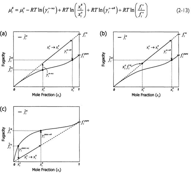
com-ment on why the standard state activity coefficients are present. Consider equation (2-13), which is a combination of equations (2-3) and (2-7). Equation (2- 13) is also demonstrated

graphically in Figure 2-2(a) and (c) for a two-component mixture of solute and solvent, us-ing both the infinite-dilution and ideal solution reference behaviors.

pl7

=/qPO -RTln

_{(•-o)+ RTln}

_(x)+

_{+RTln(7y R)+ RTln}

_fi,

Mole Fraction (x,)

(c)

, (b) f pure Mole Fraction (x,) f pure Mole Fraction (x,)

Figure 2-2: Schematic representation of the steps needed to convert from the standard state to the actual state. (a) Steps to convert from a real standard state to an actual state using the infinite-dilution (Henry's Law) reference behavior. (b) Steps to convert from an idealized standard state to an actual state using the infinite-dilution reference behavior. The idealized standard state is determined by extrapolating dilute-limit behavior to higher mole fractions. (c) Steps to convert from a real standard state to the actual state using the ideal solution reference behavior.

Essentially, a path must be found to convert from the known standard state chemical po-tential to the unknown actual state chemical popo-tential, which are related to the fugacity. This path can be thought of as a thermochemical cycle from the standard state fugacity to the actual state fugacity, as shown in Figure 2-2(a) or (c). This example cycle is based on a single species, but it is straightforward to extend this concept to a reaction. The cycle

be-(a)

-tM

U_

ir

u. (2-13)

fp

fpure

gins with the chemical potentials under the standard state conditions, with the

correspond-ing fugacities of each species, .o. The process is composed of three steps:

(i) The first step removes the non-idealities present at the standard state

condi-tions. This step reverts back to reference behavior line, and is accomplished

with the -RT In(y (7") term shown in equation (2-13).

(ii) The next step in the cycle adjusts for differences in the composition at the

stan-dard and actual states and is accounted for by the +RTln ýK term.

(iii) The final step in the process converts from the reference behavior to the actual

behavior at the composition of the system as given by the +RTln(y+-#)

term.

The final term, RTln(f+/ f +) , was left in for completeness and would be zero when the

reference behavior is chosen to be the same for the actual and standard states for the molecule of interest. Examining the situation graphically and as a cycle brings up an inter-esting point about what is required when defining the standard state chemical potential or

free energy change. Although the work here assumes that AG, includes all non-idealities,

making it a "true" free energy change under the standard state conditions, one should real-ize that other standard state free energy definitions are possible. As in the Henry's Law experiments or computational chemistry calculations, it may be much easier to obtain thermochemical properties under very dilute conditions, ignoring non-ideal effects. It is also possible to extrapolate the dilute-limit behavior (or ideal solution behavior) to

concentra-tions well beyond where this limit is applicable. If this is done, one is left with a fugacity

es-timate that ignores non-idealities at mixture conditions that do not justify this simplification. The result is a fugacity that lies on the reference behavior line, as indicated by the xof," fugacity in Figure 2-2(b). In this case, a measurement would have been made under

infi-nite-dilution conditions and extrapolated to x_i = x0. If this type of standard state data is

used, one must simply ignore the standard state activity coefficients because the standard state fugacity already lies on the reference behavior line and does not need a correction. Steps (ii) and (iii) of the cycle are the same as described above. The point to take away

here is that the standard state is arbitrary and can be defined in a variety of ways; however, one needs to be sure of exactly what assumptions are implicit in the equations and data being used. The unfortunate fact is that one rarely knows whether the data being used was measured or calculated at the standard state concentration, or measured or calculated at some other condition and extrapolated using a set of assumptions. This example illustrates one method for obtaining equations for solution-phase equilibrium constants. Each as-sumption was addressed in turn, and it is left up to the user to decide those that are legiti-mate for a system under scrutiny.

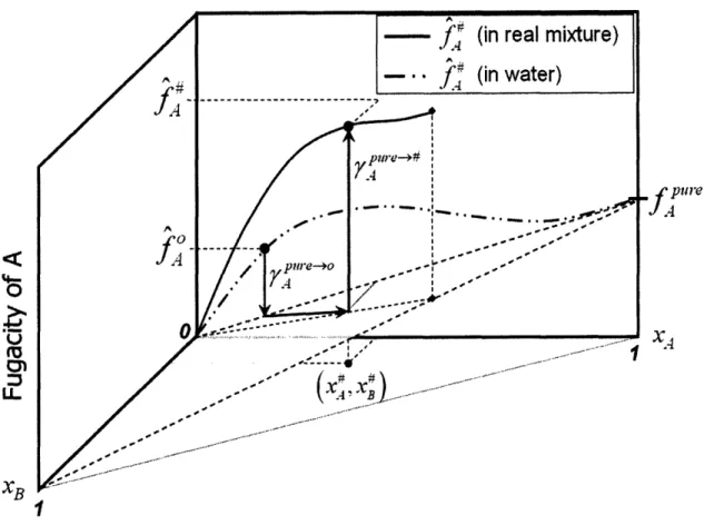
The above figures assume that the system is only composed of two molecules, the solute and solvent. However, most systems of practical importance are much more complicated multicomponent mixtures. Everything covered earlier is still valid, but there is additional complexity in understanding the process. A schematic similar to what was shown before for the fugacity cycle is given in Figure 2-3 for a solution of A, B, and water. This figure shows the case where the standard state is taken to be some concentration of A in water (no B present), as is often the case with measured data. The cycle is very similar to the two-component case, but when the concentration of A is changed from x - x~ the concentration of B must be changed from 0 -* x4 and the concentration of the solvent must be changed accordingly. All of these changes occur under the reference behavior conditions for A, so equation (2- 13) is still valid because the reference behavior for A is only dependent on the concentration of A. The final step of the process involves including the appropriate interactions between A, B, and the solvent in the real mixture, which are captured by the activity coefficients, y7". Therefore, although multicomponent mixtures are more complicated, conceptually they are very similar to a single-solute, single-solvent system. The governing equations are also identical, and it is only the activity coefficient that is more complicated and likely more difficult to estimate accurately.

Q6

Cn~

u.

X,-Figure 2-3: Graphical representation of the process to transition from the standard state fugacity in water to

the actual state fugacity for molecule A in a mixture of A, B, and water.

2.3

Practical Equilibrium Expressions

The methodology discussed above can also be used to develop equilibrium relationships between gaseous and condensed phases. Specific vapor-liquid equilibrium relationships can be derived from the general expression by making further assumptions. The general VLE relationship can be obtained from equation (2- 10), realizing that VLE is essentially an equi-molar reaction transferring the same molecule from one phase to another. Furthermore, the gas-phase mole fraction is written as a partial pressure (pi) and the activity coefficient as a fugacity coefficient. A general expression for the standard state solvation energy in terms of the compositions and behavior of the two phases is obtained, as shown in equation (2-14). Here, O,".P is the fugacity coefficient that accounts for gas phase non-idealities and is analogous to the activity coefficient for condensed phases. It was assumed that the

gas-phase reference state was a pure ideal gas at the temperature and pressure of the system

(fi = yP Yi' P) .

f pure_JA

KA = Xp

A>

RT

oOi -0 (2- 14)

'ixr

,,

It is relatively straightforward to define the Henry's Law and vapor pressure relationships by applying additional assumptions to the general equation. A relationship between the

Henry's Law constant and the solvation energies can be obtained by making the following assumptions: the solution-phase reference state is based on Henry's Law behavior, the actual solution-phase concentration is very small (y0+# 1), and the gas phase behaves ideally under

all conditions (0-+# = #+-M = 1). This allows one to arrive at equation (2-15) when H - p,/x, and y " _{is the activity coefficient correction under standard state conditions} in the condensed phase. The value of AGooV depends on the choice of the standard states for both the solution phase and the gas phase, which are typically different.

H =

r

x0 -( O jo -exp AG(oI RT (2-15)

The vapor pressure relationship is derived by applying the following assumptions: the mole fraction of the condensed phase is one, the reference state is based on ideal solution

be-havior (yfure# = 1), and the vapor phase behaves ideally. The result is equation (2-16)

describing the vapor pressure as a function of the solvation energy. You can see that the equation is identical in form to Henry's Law but based on a different reference behavior, which should be expected given that they both describe VLE in opposing limits. The two reference behaviors results in different activity coefficients for a given standard state com-position, causing a difference between H and p'aP for a given value of AGv,.

The activity coefficient needed to relate the standard state and reference state behaviors continues to be a problem because it is typically difficult to estimate accurately. To exacer-bate the problem, a typical standard state of I M will often not obey the dilute or ideal so-lution behavior taken as the reference, making estimation of the activity coefficient a neces-sity. The other option is to use a solvation free energy value that is based upon the refer-ence behavior (not the actual behavior) at the standard state concentration, which will be

denoted AGI'_{. For example, extrapolation of the dilute-limit solvation energy (AGS,,)}

to the standard state concentration will yield a standard state concentration solvation

en-ergy based on dilute-limit behavior, AG.0 •. If this data was available and used in place of

AGO in equation (2-15), then the y•",o term would not be needed because the

correc-tion to the reference behavior has already been made by using AGO". A similar concept

can be applied to the vapor pressure expression. Equations (2-15) and (2-16) can be re-written in terms of the idealized standard state solvation free energies, as shown in equa-tions (2-17) and (2-18).

H= r oX .exp -Go (2-17)

ap ( OR

y

X ) RTT

2.4

Solution-phase Transition State Theory

Transition state theory (TST) is a commonly employed approximation used to estimate gas-phase rate constants from ab initio quantum chemical calculations. The solution-phase analog is a straightforward extension based upon the equilibrium relationships derived above, which means that it is plagued by the same confusion and ambiguity. This section will discuss the solution-phase TST equations, the approximations often made, and where

confusion can arise. A bimolecular reaction will be examined: A + B " TS -- Products.

case, then one would require that additional coefficients, i"+- and ,+s", be present to account for gas-phase non-idealities as a function of the composition, pressure, and

tem-perature that affect the solvation energies.

The general expression for the TST rate constant can be seen in equation (2-19), where

Kc is the equilibrium constant between the reactants and the transition state (TS), K is

the statistical/tunneling factor, kB is Boltzmann's constant, h is Planck's constant, and T is

temperature.9

kTST = K _h Kc (2-19)

The typical procedure for a gas-phase reaction would be to write the equilibrium constant as a ratio of partition functions. This could be done for a condensed-phase reaction, but it may be more illustrative to use previously-derived expressions for Kt in terms of free

en-ergy changes. Using a similar form as equation (2- 12), the TST rate constant can be

writ-ten in terms of the free energy change of reaction, activity coefficients, and the standard state composition. This is shown in equation (2-20) where all applicable terms are based upon the solution-phase standard state. As before, the final term involving the total solu-tion concentrasolu-tions can often be neglected and is neglected in all subsequent equasolu-tions.

kT = kT exp

rsr

h

-AGsson_TS,soln RT _{.( °A B)} C9CI (y -o +- -# V * ±-41 c0 C

O

YTS 7A YB TA T,B

+# V4o B+-o C ,COs

7TS YA YB T T, TS

It is possible to connect the solution-phase expression to the more common gas-phase

form. First, AGssoIn is split into the gas-phase free energy change at an arbitrary gas-phase

standard state and the change in solvation energy for the reaction. The solvation energy change is defined in equation (2-22), where each solvation energy is defined for the

proc-ess of transferring a molecule from the gas-phase standard state (C gs) to the condensed

phase at the solution-phase standard state (CI,soln). The result is equation (2-2

1).