HAL Id: inria-00331914
https://hal.inria.fr/inria-00331914
Submitted on 20 Oct 2008
HAL is a multi-disciplinary open access
archive for the deposit and dissemination of
sci-entific research documents, whether they are
pub-lished or not. The documents may come from
teaching and research institutions in France or
L’archive ouverte pluridisciplinaire HAL, est
destinée au dépôt et à la diffusion de documents
scientifiques de niveau recherche, publiés ou non,
émanant des établissements d’enseignement et de
recherche français ou étrangers, des laboratoires
Geometry Textures and Applications
Rodrigo de Toledo, Bin Wang, Bruno Lévy
To cite this version:
Rodrigo de Toledo, Bin Wang, Bruno Lévy. Geometry Textures and Applications. Computer Graphics
Forum, Wiley, 2008, 27 (8), pp.2053-2065. �10.1111/j.1467-8659.2008.01185.x�. �inria-00331914�
Geometry Textures and Applications
†
Rodrigo de Toledo1and Bin Wang2and Bruno Lévy3 1Tecgraf – PUC-Rio, Rio de Janeiro - RJ, Brasil 2School of Software, Tsinghua University, China 3INRIA – ALICE, Villers-lès-Nancy, France
Abstract
Geometry textures are a novel geometric representation for surfaces based on height maps. The visualization is done through a GPU ray casting algorithm applied to the whole object. At rendering time, the fine-scale details (mesostructures) are reconstructed preserving original quality. Visualizing surfaces with geometry textures allows a natural LOD behavior. There are numerous applications that can benefit from the use of geometry textures. In this paper, besides a mesostructure visualization survey, we present geometry textures with three possible applications: rendering of solid models, geological surfaces visualization and surface smoothing.
1. Introduction
A set of geometry textures can be used to represent com-plex surfaces as an alternative for triangle mesh representa-tion [dTWL07]. The goal is to interactively display finely tessellated geometric models. Geometry texture visualiza-tion is implemented on the GPU and the main rendering ef-fort is on the pixel pipeline. Transferring the workload to the pixel pipeline brings the benefit of a natural LOD, since rendering time is proportional to the number of rendered pix-els. Therefore, when a complex object is far away from the viewer, less computation must be done.
The main idea in our technique is to reconstruct the fine-scale geometric details over a simple proxy of the original model. Fine-scale geometric details are known in the litera-ture as mesostruclitera-tures. Mesostruclitera-tures are commonly simu-lated as a pattern in visualization systems. In a different sit-uation, we want to reconstruct the complete object. In our case, the mesostructure changes along the object surface, and memory becomes an issue. For this reason we are in-terested in height maps, which are a compact way to repre-sent surfaces. The input of our rendering technique is a set of height maps generated from the original model to represent
† This paper is based on Geometry Textures, by Rodrigo de Toledo, Bin Wang, and Bruno Lévy, which appeared in th eProceedings of SIBGRAPI 2007 - XX Brazilian Symposium on Computer Graphics and Image Processing.
the real geometry information. We directly use the maps dur-ing renderdur-ing, executdur-ing a ray-castdur-ing algorithm on the GPU. In our approach, the geometry is passed to the GPU as a tex-ture (the geometry textex-ture), which is used by the fragment shader. Geometric details are reconstructed with the correct shading, self-occlusion and silhouette.
There are many applications that can benefit from visu-alization with intrinsic LOD behavior. We have investigated two of them: complex solid objects rendering and geological surfaces visualization. In the first one, models are partitioned to produce several geometry textures. On the second appli-cation, we are able to visualize a set of geological horizons, each one rendered as a geometry texture. Finally, we also re-search a third application that make use of image operations on geometry textures to smooth detailed surfaces.
The remaining of this paper is organized as follows: • Section 2 classifies major work on mesostructure
vi-sualization according to how the techniques represent mesostructures. We conclude by demonstrating the reason for choosing height maps as our mesostructure represen-tation.
• In Section3, we discuss previous work that also use a set of height maps to represent and render solid models. • The basic rendering algorithm for geometry textures is
ex-plained in Section4.
• Section5presents how to convert complex solid models into our geometry-texture representation.
c
The Eurographics Association and Blackwell Publishing 2008. Published by Blackwell Publishing, 9600 Garsington Road, Oxford OX4 2DQ, UK and 350 Main Street, Malden,
• Then, Section6describes three possible applications for our technique.
• Finally, in Section7, we draw some conclusions and dis-cuss different future work.
2. Mesostructure
The appearance of an object is a result of the microstruc-ture in its surface. A complete model that takes into account the microstructure and all the physical events occurring in this scale would be impractical and far from interactive rates. For this reason a lot of effort was dedicated in representing the appearance in a mesoscale level, between the micro and macro scales. The surface structure we need to represent in this level is named mesostructure.
When touching an object, one can feel its texture. Actu-ally, textures give both tactile and visual information in such a way that we can imagine the sensation of touch by just looking at an object. The texture is a result of the object mesostructure and it can be simulated in several ways in vi-sualization systems. Its simplest representation is the color map, which is a simple 2D image applied over a virtual ob-ject [Cat74,BN76]. Blinn extended texture mapping with the bump mapping technique [Bli78], which gives visual effects of bumps and depressions by disturbing surface normals ac-cording to a bump map.
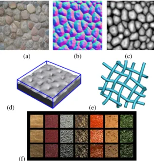
More complex mesostructure representations store meso-information in other formats: height maps, volume data, shading functionsand polygonal meshes (see Figure1). We describe some major work in the following sections.
2.1. Height-map mesostructure
The first technique that used a height map to represent and render mesostructures was displacement mapping [Coo84]. It subdivides the macro geometry into a large number of small polygons whose vertices are displaced in the normal direction according to the associated displacement map. Its drawback is the excessive number of generated polygons.
To avoid extra polygons, the VDM method (View-dependent Displacement Mapping [WWT∗03]) adopts the idea of previously sampling mesostructure appearance un-der various lighting and view directions. In preprocessing, a height map is taken as input and synthesizes a set of VDM images for different view directions and different curvatures, recording the VDM data as a 5D function. Although result-ing in good quality, this method transforms a 16KB map into a 64MB volume of data, which prevents its application for our purpose, since we use hundreds of maps.
Policarpo et al. [POC05] use height maps to interactive mesostructure visualization. Their method is the most sim-ilar to ours, using GPU ray casting. However, they do not devote attention to complex and highly-tessellated surfaces.
(a) (b) (c)
(d) (e)
(f)
Figure 1: Different representations for mesostructures: (a) color maps, (b) normal maps, (c) height maps, (d) volumetric mesostructure [CTW∗04], (e) polygonal mesh [ZHW∗06], and (f) shading function (picture from Columbia University website).
Hirche et al. work [HEGD04] is also centered in a height-map ray-casting per-pixel implementation. However, they extrude some prisms from the base mesh (their macro-geometry), and the ray casting is done by using the prism walls, quadrupling the number of faces, which is unneces-sary in our method.
2.2. Volumetric mesostructure
The use of volumetric mesostructure brings a more flexible way to represent details. The mesostructures found in real world are better approximated by volumes, which have no overlapping restriction. Another advantage is the possibility to add opacity per-voxel information, which can be used for simulating more complex lighting phenomena as refraction and subsurface scattering.
Most of the rendering applications use prism extrusion from the base mesh to create a 3D parameterized space. This can lead to self-intersections near concave features, which is solved by some methods [PKZ04,PBFJ05].
In Lensch et al. work [LDS02] volumetric textures are ap-plied over arbitrary macro-geometry mesh. They use back to front slicing technique, drawing the polygons inside each prism formed by the intersection of the orthogonal viewing slices. To produce a fast intersection computation, they have created a structure based on normal edge classification. So,
the slices are rapidly computed. They have created 3 differ-ent implemdiffer-entations: in software, in hardware, and a hybrid one, which is the fastest.
Wang et al. work [WTL∗04] is a generalization of VDM that accepts volume mesostructure definition. Their main structure, named GDM (Generalized Displacement Maps), is also a five-dimensional function accessed in real-time, but as opposed to VDM they use prisms, computing the ray exit point and evaluating the intersection in each prism domain.
In Shell Texture Function (STF [CTW∗04]), Chen et al. compute subsurface scattering, using photon tracing in pre-processing and ray tracing for final visualization, but the ren-dering are not interactive (images are generated in about 100 seconds). In their subsequent work, SRTF (Shell Radiance Texture Functions) [SCT∗05], the visualization achieves in-teractive frame rates. However, it is not possible to reproduce detailed silhouettes since SRTF is rendered without ray trac-ing. Indeed, these techniques are a hybrid approach between ray casting and shading functions (described in Subsection
2.4).
2.3. Polygonal mesostructure
Zhou et al. [ZHW∗06] have developed interactive good re-sults by rasterizing polygonal mesh mesostructure. They carefuly stitch together geometry elements finding corre-sponding elements in adjacent mesostructures patches. They succesfully align elements through local deformation al-though presenting some distortion on regions with very high curvature.
In contrast to Zhou et al. work, Shell Maps [PBFJ05] do not render the final geometry. They create prisms arround the surface (similar to some previously mentioned techniques) and map them on their counterpart prisms in texture space. They create a general procedure to ray cast mesostructures in texture space. Although the possibility to apply their pro-cedure for different mesostructure representations, in their examples they use polygonal and procedural ones, rendered in non-interactive rates.
2.4. Representations of the Shading Function
Shading models are a very complex and important subject in visualization domain. Its complexity comes from the fact that these models try to represent and simulate the lighting phenomena happening in microscale level to obtain results in macro and mesoscale levels. Generally, in interactive appli-cations, the shading model in use is the diffuse/specular one, which is only an approximation of real lighting effects. For more accurate shading, a bidirectional reflection distribution function(BRDF) is more appropriate to categorize how light is reflected from a point on the surface.
BRDF= f (θin, φin, θout, φout) (1)
So, based on the BRDF model, to compute the outgoing light Loin a given direction ~ωowe need to integrate the
in-coming light in all directions:
Lo(~ωo) =
Z
Ω
BRDF(~ωi,~ωo)Li(~ωi)cos(θi)d~ωi (2)
where Ω represents the hemisphere vectorial space since the light beams coming from the back are not considered. ~ω de-scribes the spherical coordinate angles (θ, φ) of a given di-rection vector.
This subsection covers the methods based on BRDF prin-ciples. Most of them use a set of images as the input informa-tion about the mesostructure shading funcinforma-tion. This image collection is the result of capturing real pictures of the de-sired materials from different points of view, uniformly dis-tributed in a hemisphere. In some methods [LYS01,VT04] this is done synthetically.
Dana et al. [DvGNK99] introduced BTF (bidirectional texture function) in an experimental work based on the BRDF principles. They captured a set of images, using dif-ferent material samples and varying the light and viewing directions. The images are stored in a publicly available database. So, the BTF is a 6D function, which has the same 4 BRDF variables (Equation1) plus 2 for position on the image:
BT F= f (θin, φin, θout, φout, u, v) (3)
Some methods have extended the BTF approach. Liu et al. [LYS01] address two related problems: the synthesiza-tion of a continuous BTF and the specificasynthesiza-tion of new syn-thesized BTF’s without the captured images. In [TZL∗02], Tong et al. succeeded in rendering arbitrary surfaces with BRDF material although in low speed (about 1 frame per second).
Applying BTF on surfaces for real-time rendering is not easy; the lookup value at (u, v) is a hard task since BTF original information consists of a large amount of images. Polynomial Texture Maps[MGW01] is a BTF simplification since it removes the viewing direction from the equation, re-ducing the number of images taken for each surface.
PT Mr,g,b(θin, φin, u, v) (4)
Instead of recording and accessing all the pictures, which would still be very costly, they do a convenient approxima-tion to store texel informaapproxima-tion: split chromaticity per-texel luminance approximated as a biquadratic expression.
TensorTexture [VT04] technique uses synthetic mesostructure. It also differs from BTF in storing in-formation. It applies a dimensionality reduction after a
multilinear analysis of the image data tensors. However, this approach had proved to be too slow for interactive rendering. The CPU implementation has an average time of 1.6 seconds per image.
2.5. Comparing mesostructure techniques
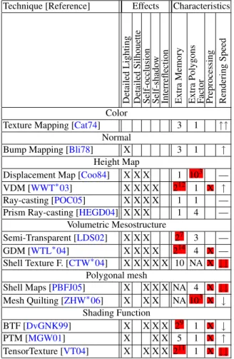
Technique [Reference] Effects Characteristics
Detailed Lighting Detailed Silhouette Self-occlusion Self-shado w Interreflection Extra Memory Extra Polygons F actor Preprocessing Rendering Speed Color
Texture Mapping [Cat74] 3 1 ↑↑ Normal
Bump Mapping [Bli78] X 3 1 ↑ Height Map
Displacement Map [Coo84] X X X 1 103 — VDM [WWT∗03] X X X X 212 1 X ↑ Ray-casting [POC05] X X X X 1 1 — Prism Ray-casting [HEGD04] X X X 1 4 —
Volumetric Mesostructure Semi-Transparent [LDS02] X X X 27 3 — GDM [WTL∗04] X X X X 214 4 X — Shell Texture F. [CTW∗04] X X X X X 10 NA X ↓↓ Polygonal mesh Shell Maps [PBFJ05] X X X X NA 4 X ↓↓ Mesh Quilting [ZHW∗06] X X X NA 103 X ↓ Shading Function BTF [DvGNK99] X X X X 29 1 X ↓ PTM [MGW01] X X X 5 1 X ↑ TensorTexture [VT04] X X X X 211 1 X ↓↓ Table 1: Comparison between different interactive mesostructure visualization. Negative points are marked with a red background.
We summarize the visual effects and characteristics of some of the main mesostructure visualization techniques in Table1. Some of the presented numbers are approximations, but they are meaningful to compare different techniques. For example, in Extra Memory, we have evaluated how much per-texel information is needed to represent the mesostruc-ture (computing the uncompressed data). Preprocessing marks those that present expressive pre-computations. In Rendering Speed column, up arrows mean fast rendering while down arrows mean slow rendering (no arrows are used for average speed).
Based on Table1we decide to use height-map ray-casting
algorithm for mesostructure rendering. It is the best option in number of visual effects that do not contain significant negative points (those in red boxes).
3. Related Work on Multiple Height Maps
The use of multiple height maps for representation of a com-plex model is an interesting idea due to the compactness. For rendering, the use of GPU height-map primitives is promis-ing. The drastic reduction of vertices in the scene (the usual bottleneck for complex object visualization) may result in better performance. On the other hand, the GPU height-map primitives visualization converges the effort in the pixel shader. For this reason they have a natural LOD behavior. In this section, we describe some work previously done that are related to this approach.
RTM (Relief Texture Mapping [OBM00]) is the first work on object visualization based on multiple height maps. RTM starts by capturing the depth of an object from six orthogonal points of view. In rendering time, a warping-based technique is applied on the faces of the bounding box to reconstruct the original model.
Badoud and Décoret [BD06] use multiple height maps to represent and render complex objects. They store the height maps of the six orthogonal points of view using an adapted perspective frustum, which increases the detail information about features that are almost perpendicular to the view point. During rendering, they use a clipped frustum to re-duce the number of discarded fragments.
Porquet et al. [PDG05] have developed a technique to ren-der complex surfaces by using a rough geometric approxi-mation on which colors and normals are applied according to previously captured information, including height maps. In preprocessing, they capture the maps from several points of view. In rendering time, the three closest views to the cam-era projection are used by the fragment shader. Based on the height maps, the fragment shader reconstructs the equivalent information of the three points of view to finally find which one is the nearest sample to the current fragment, defining the color and the normal to be used. The main disadvantage of this method is the lack of silhouette details.
The multi-chart geometry images method [SWG∗03] is similar to our geometry textures method, although it does not use height maps. It extends Geometry images [GGH02] by splitting a model into multi charts before parameterizing each one onto a square. It is especially different from our method during rendering. To render the geometry images, it is necessary to reconstruct many triangles from the images, overcharging the vertex pipeline, which is exactly what we want to avoid. Since geometry image patches are defined on the surface itself rather than height maps, they cannot apply any optimization at the GPU fragment shader.
4. Geometry Texture Rendering 4.1. Height-map GPU ray casting
A height map (a.k.a. height field, relief map or depth tex-ture) is a 2D regular table where a height is specified for each entry. One way of representing a height map is a grayscale image with brightness representing height (see Figure1(c)). Terrains are an example of a surface well suited to be repre-sented by height maps.
A height map can be represented by the function:
hm(x, y) : [0, 1]2→ [0, 1].
We can define a Boolean function z(P), for (P.x, P.y, P.z) ∈ [0, 1]3, as:
z(P) ⇐ ( P.z ≤ hm(P.x, P.y) ) ? true : false, In our implementation, we use the faces of a paral-lelepiped to generate the fragments that will ray cast the height map. The coordinates of its vertices are between 0 and 1 (as in a canonical cube), defining the local coordinate space. The height map data is passed to the GPU through a grayscale texture. The x and y axes of the parallelepiped are exactly coincident with the u and v coordinates of the texture, while z coincides with the height direction.
In GPU, the vertex shader sends to the fragment shader the viewing direction already in local space. This way, each fragment knows the path of the ray inside the canonical cube, and can easily compute its exit point. The fragment-shader’s main task is to answer the two ray-casting questions: is there an intersection between the ray and the height map? Where is the closest hit point?
As explained in [POC05], one strategy is to uniformly sample this ray path in N points Piand use function z(P) to
find the ray-surface intersection. This could be implemented by a conditional loop varying Pi, from the entering to the
exit point, and stopping when z(Pi) is false. In each step Pi
is translated by ∆, which is the ray path divided by N. When a ray does not intersect any height sample, the frag-ment should be discarded without any contribution to the frame buffer or to the z-buffer. For fragments not discarded, the actual color can be retrieved from a color texture, and the normal can be either computed directly from the height map or given as a third texture to be used for shading. The co-ordinates used in the texture lookup are (P.x, P.y) right after the iterations. Finally, the depth is computed to register the correct z-value for the z-buffer.
Two-step searching. Even if ∆ is short enough not to miss a sample, the point where the ray touches the object is not exactly computed. As proposed in [POC05], we use a second searching step between points Pi−1and Pi. This second step
is a binary search that divides the searching domain by two
in each step. Therefore, with M steps in the binary search we multiply the precision by a 2Mfactor. Notice that this second searching procedure is done in the same fragment code, it is not a multi-pass algorithm.
We propose the following improvements for the height-map GPU visualization:
Non-rectangular height map domain. A height sample with value equal to 0 can be considered either as the surface base or as a representation of empty space. We have chosen the last case, since representing empty space is essential for geometry textures. Figure4(d) has an example.
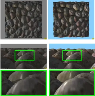
Balancing between steps. Binary search is much more ef-ficient than linear search. However, it cannot be exclusively executed because, along the ray path, there could be several intersections. In other words, the z(P) function may change different times along the parametric ray for each fragment. On the other hand, when the ray is totally perpendicular to the height map (in a perfect top view), z(P) will change sign at most once. In this case, the binary search can perfectly and efficiently compute the intersection without the previous lin-ear slin-earch. Based on this observation, we have implemented a balance between the linear and the binary steps according to the viewing slant. When in a vertical view, we reduce the linear search iterations while increasing the binary search iterations (N↓, M↑). For an almost horizontal viewing direc-tion we do the opposite, prioritizing the linear search (N↑, M↓). This way, we achieve up to two times faster rendering for some cases (see Figure2) than without balancing.
Some other methods were proposed to accelerate GPU ray casting of height maps [Don05,PO07]. However, they need extra information about distance functions.
4.2. Geometry Textures
The problem approached in our work is different from stan-dard mesostructure rendering. We are interested in recon-structing the details of an entire object, which is a non-repetitive pattern, since it changes over the model domain. In our case, the input is a set of height maps converted from the original model to represent the complete geometrical in-formation.
Geometry texture is a geometric representation for sur-faces. Its domain is a parallel hexahedron and in its interior a height-map represents the surface (see Figure3). The do-main is not restricted to a perfect rectangle, so empty sam-ples are expected in each geometry texture. The construc-tion of geometry texture patches from a complex model has no global folding restriction and the patches are well fitted around the surface contour. In rendering time, geometry tex-tures use our ray-casting algorithm implemented in a frag-ment shader. As a result, the geometry is correctly recon-structed and rendered.
Figure 2: Comparing not-balanced and balanced searches (right column). With balanced search, we obtain better per-formance (85 fps× 66 fps on a GeForce 6800) when seen from above and better quality when seen in a profile view.
Figure 3: Geometry texture sample. A height map defined inside a hexahedron’s domain.
5. Conversion
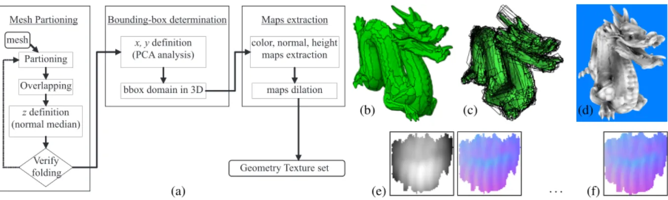
The input for our conversion procedure is a polygon mesh and the output is a set of geometry textures. There are three main steps when converting triangle meshes into geometry textures (see Figure4(a)): mesh partitioning, bounding-box determination and maps extraction.
Among the three conversion steps, mesh partitioning is the most difficult and critical for the success of the algo-rithm. Some conditions are expected when partitioning the input model mesh into charts:
• The chart must not contain a folding situation in its~z. • The chart domain should be as square as possible to
re-duce empty spaces.
• For visualization purposes, neighboring charts must share
their boundary, resulting in some overlapping between them. Right after partitioning we add an extra triangle ring around each chart (see Figure4b). As explained in
[dTWL07], the overlap area is necessary to avoid cracks,
while in rendering time, z-buffer information is correctly generated to achieve a seamless reconstruction.
Bounding-box determinationincludes finding a good or-thonormal coordinate system and domain for each one of the charts. Direction ~z is taken as the median normal of all tri-angles in one chart, with this we minimize the occurence of self-folding partitions. Then, ~x and ~y must be chosen based on the minimization of empty spaces in the domain. We have used the 2D-PCA (Principal Component Analysis) algorithm to determine directions ~x and ~y projected on the plane defined by ~z. Finally, we project the coordinates of all triangles to obtain the exact domain in each direction. (~x,~y,~z) forms the local coordinate system of the chart.
In the map extraction phase, there are three maps we want to obtain: height, color and normal maps. We have devel-oped a GPU solution to extract the three maps from one chart. Based on the local coordinate system of each chart, we render its triangles in an orthogonal view projection per-pendicularly to direction ~z, filling out the viewport with a user-defined resolution (for example, 256 × 256). We repeat the procedure three times capturing the image buffer: • To obtain the color map we render the colors without
illu-mination.
• To generate the normal map we assign (x, y, z) global co-ordinates of normal ~niof each vertex vito (r, g, b). During
rasterization, within each triangle, the normals are inter-polated and then normalized again.
• To obtain the height map we start by finding in CPU the maximum and minimum coordinates (hmax and hmin) in
direction ~z. We assign a value hi∈ [0, 1], computed as
hi=hvmaxi.z−h−hminmin, to each vertex vi. This value is interpolated
inside the triangles and outputted as luminance.
Note that for space-reduction purposes, the image buffer is captured and stored using 8-bit precision.
The rendering algorithm loads the maps as textures. How-ever, before that, we apply a texel-dilation procedure to pre-vent sampling problems when using mip-mapping. These problems may occur when the graphics hardware access bor-der information for non-rectangular domain, using a null value (from out of the domain) to interpolate the returning value. Our dilation algorithm fills empty texels around the map domain with interpolated values. The procedure is done for normal and color maps. See Figure4.
In the following subsections we discuss two different strategies we have implemented for mesh partitioning: PGP (Periodical Global Parameterization [RLL∗06]) and VSA (Variational Shape Approximation [CSAD04]).
Mesh Partioning Bounding-box determination Maps extraction Partioning Overlapping Verify folding z definition (normal median) x, y definition (PCA analysis) bbox domain in 3D
color, normal, height maps extraction
maps dilation
Geometry Texture set mesh (a) (b) (c) (e) · · · (d) (f)
Figure 4: (a) Complete procedure for converting polygon meshes into a set of geometry textures. (b) Mesh partitioning. (c) Bounding-box determination. (d) Height-map extraction (e) Height and normal maps of a patch. (f) Map dilation (two-pixel dilation).
5.1. Partitioning with PGP
Periodic Global Parameterizationis a globally smooth pa-rameterization method for surfaces. PGP can be applied to meshes with arbitrary topology, which is a restriction in other parameterization methods [RLL∗06]. Moreover, we can extract a quadrilateral chart layout from this parameter-ization, which is based on two orthogonal piecewise linear vector fields defined over the input mesh. This orthogonality is especially interesting to guide our partitioning procedure in order to reduce empty spaces in the domain. These vec-tor fields are obtained by computing the principal curvature directions, resulting in a parameterization that follows the natural shape of the surface (left picture on Figure5).
PGP avoids excessive empty spaces. However, often charts obtained with PGP partitioning present some fold-ing problems. For this reason we have decided to investigate VSA as an alternative partitioning method.
5.2. Partitioning with VSA
Variational Shape Approximationis a clustering algorithm for polygonal meshes that can be used for geometry sim-plification [CSAD04]. Our partitioning algorithm based on VSA uses each cluster as an initial chart, which is further increased to overlap neighboring domains (see Figure4).
The main advantage of using VSA compared to PGP is that it reduces the number of folding cases. VSA uses L1,2 metric, which is based on the L2measure of the normal field. This means that it takes into account the normal direction of the vertices to cluster them. A folding situation occurs only if vertices in a chart have a sharp difference in their normal direction (over 90 degrees). With VSA, each chart only contains vertices with similar normal directions.
In the next section we describe some experiments to com-pare the PGP and the VSA methods.
5.3. Comparing PGP and VSA
In our tests we have partitioned with both PGP and VSA two different models: bunny and buffle (Figure5).
Our first test compares how good PGP and VSA are at avoiding empty spaces. We have counted for each chart the number of used and empty texels. This was done in the four test cases (PGP bunny, VSA bunny, PGP buffle and VSA buffle). For simplicity, the charts were extracted with-out overlapping and the maps withwith-out dilation. The maxi-mum map size was 128 × 128. A map could be smaller than that (adapted to the chart size), as long as each dimension remained a power of two (respecting OpenGL’s restriction). Table2shows the results, indicating that PGP is better at avoiding empty spaces.
Model Method Total texels Empty texels % Bunny PGP 1008128 240357 23.84% Bunny VSA 461312 179194 38.84% Buffle PGP 2498048 563652 22.56% Buffle VSA 979456 453069 46.25% Table 2: Considering empty spaces, PGP is better than VSA.
In our second test we have counted how many charts have folding problems, again in the four test scenarios. A way to check if a chart has a folding situation is to verify if there is any inverted triangle when rasterizing all triangles in lo-cal direction ~z. Given that the triangles in the mesh respect a counterclockwise rotation, if at least one of them is ras-terized clockwise then the mesh folds itself in direction ~z. Figure5shows a partitioned buffle model with inverted tri-angles marked in green. In Table3we present the number of folding charts and the total number of inverted triangles found. Clearly, VSA is more appropriate to avoid folding problems.
Figure 5: Buffle partitioning with PGP and with VSA. Triangles with folding problem have their vertices marked in green.
Model Method Initial Initial Inverted Folding triangles charts triangles charts Bunny PGP 69,451 224 817 45 Bunny VSA 69,451 222 3 3 Buffle PGP 117,468 403 2819 62 Buffle VSA 117,468 397 34 6 Table 3: VSA significantly reduces the number of folding charts (identified by inverted triangles).
While PGP is better for reducing empty spaces, VSA is much more efficient in avoiding self-folding charts. We con-sider that the folding problem is the most important issue. Self-folding charts cannot be represented by our geometry texture, which is a strong restriction. On the other hand, empty-space reduction is merely an optimization.
Based on these facts, we have chosen VSA as our par-titioning method. The results presented in the next section have been achieved using VSA.
6. Applications
Once we have obtained a set of geometry textures, we can render them using the height-map ray-casting algorithm on GPU. In the following sections we discuss some applications using geometry textures visualization.
0 50 100 150 200 250 300 350 400 0 100000 200000 300000 400000 500000 600000 128x128 256x256 512x512 Mesh VBO Mesh CVA 640x480 800x600 1024x768 1280x1024
Ray-casting area in number of pixels
F
P
S
Figure 7: We have compared three different geometry texture resolutions (1282,2562,5122) and the original mesh ren-dered with VBO (Vertex Buffer Object) and CVA (Compiled Vertex Array) of the dragon model. Frame rates registered on a GeForce 8800.
6.1. Rendering of solid models
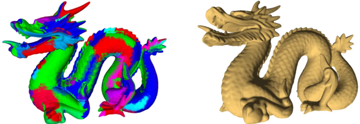
We have used the dragon model with 871,414 triangles for tests (see Figure6). We have generated three sets of 453 ge-ometry textures, varying their maximum resolution (1282, 2562and 5122). The tests were done with a GeForce 8800 GTX graphics card.
Since geometry textures have their performance bottle-necked per pixel, we have varied the zoom level in our tests. We have plotted the results in Figure7.
To compare performance between geometry textures and common triangle-mesh visualization, we have measured the rendering speed of the original dragon model in two special
Figure 6: The dragon model partitioned into 453 geometry textures and rendered with maximum resolution 256 × 256 for each patch.
situations: with Compiled Vertex Array (CVA) and with Ver-tex Buffer Object(VBO). Both methods are advanced fea-tures in OpenGL and without them the speed would be less than 1 FPS for such model size. For the dragon model with 871K triangles, we have obtained 27 FPS with CVA and 135 FPS with VBO (plotted as dashed lines in Figure7).
The horizontal axis in Figure7represents the number of pixels of the dragon’s ray-casting area, which is formed by the rasterization of the geometry-textures bounding-box faces (without recounting overlapping fragments). The higher the number of pixels, the larger the model is on the screen. For a practical idea, we have highlighted some win-dow sizes (640 × 480, 800 × 600, 1024 × 768, 1280 × 1024) which the model would fit.
The ray-casting algorithm is the same independently of resolution. However, we have verified that the lowest max-imum resolution (1282) was the fastest one. This is a result of less graphics card memory in use (4.21MB), optimizing caching and fetching. As we will see, for quality purposes, 2562 would be a good choice for maximum resolution for the dragon’s 453 geometry textures used in test. Its perfor-mance is better than the original mesh rendered with VBO for resolutions smaller than 800 × 600.
6.2. Horizons visualization
Horizons are geological surfaces representing interfaces be-tween two contiguous sediment layers. In general, horizons are extracted from volumetric seismic data [OK04]. For each seismic trace(a vertical column in the volume), at most one sample belongs to the same horizon. Thus, height maps are a natural choice to represent this surfaces, given that there is a unique representation on vertical. In oil industry, a set of horizons for one geographical region is very important to determine possible bottom and top limits of a reservoir.
Figure8shows an example of horizons set that are
rep-Figure 8: Set of horizons on the same geographical region. Each horizon is showing a different property mapped into a color scale.
resented by height-maps. To visualize them we use our ge-ometry texture technique. As a result, we obtain high perfor-mance when this set is far from the camera. Figure9presents rendering speed in three different situations: in top, profile and oblique views.
Originally, these horizons are height maps with 1588 × 1188 resolution, they could be reconstructed with about 16 million triangles. As already mentioned, the use of geome-try textures brings a LOD behavior that can be once more observed on horizons-rendering speed (see Figure9). Hori-zontal (or profile) view is not so efficient as top view because of the linear-binary balance (see Section4.1). Note that the speed values are clearly slower than in dragon example be-cause different graphics cards were used for tests.
0 20 40 60 80 100 120 0 100000 200000 300000 400000 500000 600000 700000
Ray-casting area in number of pixels
FP
S
Top
Horizontal
Oblique
Figure 9: Rendering speed of the scene in Figure8varying screen resolution in three different point of views: viewing from the top, in profile and obliquely. NVidia GeForce 7900 GTX.
6.3. Smooth surfaces
Once we have a new geometry representation based on im-ages (height maps), image operations can be applied on these maps to transform geometry . For example, one could use a low-band filter to smooth the geometry (or a high-band filter to highlight small geometric features).
We have experimented a Gaussian blur on both height and normal maps to smooth the surface. The result is a surface without most of its high frequency details as shown in Figure
10. However, it is clear that it is not possible to deliberately apply the smooth operation because each geometry-texture patch does not have complete information about the neigh-bors. As a consequence, some undesirable features start to appear on regions with strong curvature. This is not the only issue. When applying Gaussian filter with significant radius, as in Figure10(d), each patch becomes more flat and it is possible to see the seams.
7. Conclusion and Future Work
We have proposed a new representation for highly-tessellated models using a set of geometry textures, which are rendered using a GPU implementation of height-map ray casting. Our results have shown that this new representation is suitable for natural models (i.e. non-CAD models). The final rendered images have similar quality compared to tra-ditional polygonal rasterization methods.
The following items are some of the positive aspects of our technique:
• The rendering speed naturally follows a LOD behavior. This means that when the model is small on the screen (i.e., far from the camera), rendering is faster. This is a re-sult of relieving the vertex-stage burden, transferring com-putation bottleneck to pixel stage.
• Depending on the chosen resolution, our tion requires less memory than polygonal
representa-(a) (b)
(c) (d)
Figure 10: Smoothing Buffle model. (a) Original (b) 2-texels Gaussian blur (c) 4-texels Gaussian blur (d) 8-texels Gaus-sian blur.
tion, without losing significant geometry information. See
[dTWL07] for more details.
• Our technique is compatible with polygon rasterization, thus geometry-texture objects can be inserted in any vir-tual scene composed by polygonal objects.
• It is possible to apply image operations to transform model geometry.
Our potential drawbacks are:
• Recent graphics cards that implement VBO extension have very high performance for polygonal rendering. As a consequence, when compared to VBO performance, our technique is faster only if the model is not so big on the screen. However, if the scene contains multiple mod-els, polygonal rendering would proportionally lose perfor-mance, while our solution would keep a stable frame rate. • Another adverse point is the sophisticated conversion al-gorithm. Our procedure is composed by multiple passes, including the partitioning step, which is considerably elaborate. This may be improved by using multilayer height maps as shown in [SdTG08].
We suggest the following ideas for future work: Self shadows
Self shadows for height-map ray casting is a straightforward algorithm. However, in the case of geometry textures, mul-tiple maps are in use simultaneously and they do not have information about neighbor maps. Alternatively, it is always possible to use shadow mapping [Wil78] to produce
shad-ows since geometry textures keep z-buffer up to date. How-ever, shadow mapping suffers from aliasing problems and needs sophisticated algorithms to overcome this problem (see [BC07] for a survey about this subject). For this reason, ray cast for shadows, including neighboring information, is a valuable topic for future research.
Other image operations
We have implemented a simple blur operation to smooth sur-faces represented by geometry textures (Section6.3). It is possible to use other operations that may result in different geometry modifications. For example, a high-band filter can be used to highlight small geometric features. Other possible applications are operations to insert geometric patterns and simulations of cellular network [GF06].
Combined use of explicit and implicit surfaces for GPU ray casting
This work implements a GPU ray casting for height maps that uses the faces of a bounding-box to trigger the algo-rithm. This idea has also been explored for implicit surfaces rendering [TL04,dTLP07,LB06]. We suggest, as a future re-search, the combination of implicit and explicit algorithms. For example, it is possible to produce some holes in nat-ural models by subtracting some implicit spheres from the geometry texture set. Another example could be rendering implicit surface objects (e.g., a torus) applying height-map mesostructure information.
8. Acknowledgement
To Tecgraf design group. To the anonymous reviewers for their excellent contributions.
References
[BC07] BARROSOV. B. R. B., CELES W.: Improved real-time shadow mapping for cad models. In SIBGRAPI ’07: Proceedings of the XX Brazilian Symposium on Com-puter Graphics and Image Processing (SIBGRAPI 2007) (Washington, DC, USA, 2007), IEEE Computer Society, pp. 139–146.11
[BD06] BABOUDL., DÉCORETX.: Rendering geometry with relief textures. In GI ’06: Proceedings of the 2006 conference on Graphics interface(Toronto, Ont., Canada, Canada, 2006), Canadian Information Processing Society, pp. 195–201.4
[Bli78] BLINNJ. F.: Simulation of wrinkled surfaces. In Computer Graphics (SIGGRAPH ’78 Proceedings)(Aug. 1978), vol. 12, pp. 286–292.2,4
[BN76] BLINNJ. F., NEWELLM. E.: Texture and reflec-tion in computer generated images. Communicareflec-tions of the ACM 19(1976), 542–546.2
[Cat74] CATMULL E. E.: A subdivision algorithm for computer display of curved surfaces. PhD thesis, 1974.
2,4
[Coo84] COOKR. L.: Shade trees. In Proceedings of the 11th annual conference on Computer graphics and inter-active techniques(1984), ACM Press, pp. 223–231.2,4
[CSAD04] COHEN-STEINER D., ALLIEZ P., DESBRUN
M.: Variational shape approximation. ACM Transac-tions on Graphics. Special issue for SIGGRAPH confer-ence(2004), 905–914.6,7
[CTW∗04] CHENY., TONGX., WANGJ., LINS., GUO
B., SHUM H.-Y.: Shell texture functions. ACM Trans. Graph. 23, 3 (2004), 343–353.2,3,4
[Don05] DONNELLYW.: GPU Gems 2 - Per-Pixel Dis-placement Mapping with Distance Functions. Addison Wesley, 2005, ch. Per-Pixel Displacement Mapping with Distance Functions, pp. 123–135.5
[dTLP07] DETOLEDOR., LEVYB., PAULJ.-C.: Itera-tive methods for visualization of implicit surfaces on gpu. In ISVC, International Symposium on Visual Computing (Lake Tahoe, Nevada/California, November 2007), Lec-ture Notes in Computer Science, Springer, pp. 598–609.
11
[dTWL07] DETOLEDOR., WANGB., LEVYB.: Geom-etry textures. In Proceedings of SIBGRAPI 2007 - XX Brazilian Symposium on Computer Graphics and Image Processing (Belo Horizonte, October 2007), SBC - So-ciedade Brasileira de Computacao, IEEE Press, pp. 79– 86.1,6,10
[DvGNK99] DANA K. J., VAN GINNEKEN B., NAYAR
S. K., KOENDERINKJ. J.: Reflectance and texture of real-world surfaces. ACM Transactions on Graphics 18, 1 (1999), 1–34.3,4
[GF06] GOBRONS., FINCKD.: Generating surface tex-tures based on cellular networks. In GMAI (2006), IEEE Computer Society, pp. 113–120.11
[GGH02] GUX., GORTLERS. J., HOPPE H.: Geome-try images. In SIGGRAPH ’02: Proceedings of the 29th annual conference on Computer graphics and interac-tive techniques(New York, NY, USA, 2002), ACM Press, pp. 355–361.4
[HEGD04] HIRCHE J., EHLERT A., GUTHE S., DOGGETT M.: Hardware accelerated per-pixel dis-placement mapping. In Graphics Interface (2004). 2,
4
[LB06] LOOPC., BLINNJ.: Real-time gpu rendering of piecewise algebraic surfaces. In SIGGRAPH ’06: ACM SIGGRAPH 2006 Papers(New York, NY, USA, 2006), ACM Press, pp. 664–670. 11
[LDS02] LENSCH H. P. A., DAUBERTK., SEIDEL H.-P.: Interactive semi-transparent volumetric textures. In Proceedings of Vision, Modeling, and Visualization VMV
2002(Erlangen, Germany, 2002), Greiner G., Niemann H., Ertl T., Girod B., Seidel H.-P., (Eds.), Akademische Verlagsgesellschaft Aka GmbH, pp. 505–512.2,4
[LYS01] LIUX., YUY., SHUMH.-Y.: Synthesizing bidi-rectional texture functions for real-world surfaces. In SIG-GRAPH ’01: Proceedings of the 28th annual conference on Computer graphics and interactive techniques(New York, NY, USA, 2001), ACM Press, pp. 97–106.3
[MGW01] MALZBENDER T., GELB D., WOLTERS H.: Polynomial texture maps. In SIGGRAPH ’01: Proceed-ings of the 28th annual conference on Computer graphics and interactive techniques(New York, NY, USA, 2001), ACM Press, pp. 519–528.3,4
[OBM00] OLIVEIRAM. M., BISHOPG., MCALLISTER
D.: Relief texture mapping. In Proceedings of ACM SIG-GRAPH 2000(July 2000), Computer Graphics Proceed-ings, Annual Conference Series, pp. 359–368.4
[OK04] O’MALLEYS. M., KAKADIARISI. A.: Towards robust structure-based enhancement and horizon picking in 3-d seismic data. In CVPR (2) (2004), pp. 482–489.9
[PBFJ05] PORUMBESCU S. D., BUDGE B., FENG L., JOYK. I.: Shell maps. ACM Trans. Graph. 24, 3 (2005), 626–633.2,3,4
[PDG05] PORQUETD., DISCHLERJ.-M., GHAZANFAR
-POURD.: Real-time high-quality view-dependent texture mapping using per-pixel visibility. In GRAPHITE ’05: Proceedings of the 3rd international conference on Com-puter graphics and interactive techniques in Australasia and South East Asia(New York, NY, USA, 2005), ACM Press, pp. 213–220.4
[PKZ04] PENGJ., KRISTJANSSOND., ZORIND.: Inter-active modeling of topologically complex geometric de-tail. ACM Trans. Graph. 23, 3 (2004), 635–643.2
[PO07] POLICARPOF., OLIVEIRAM. M.: GPU Gems 3 - Relaxed Cone Stepping for Relief Mapping. Addison-Wesley Professional, 2007, ch. 18, pp. 409–428.5
[POC05] POLICARPO F., OLIVEIRAM. M., COMBAJ. L. D.: Real-time relief mapping on arbitrary polygonal surfaces. In SI3D ’05: Proceedings of the 2005 sympo-sium on Interactive 3D graphics and games(New York, NY, USA, 2005), ACM Press, pp. 155–162.2,4,5
[RLL∗06] RAY N., LI W. C., LÉVY B., SHEFFER A., ALLIEZP.: Periodic global parameterization. ACM Trans. Graph. 25, 4 (2006), 1460–1485.6,7
[SCT∗05] SONGY., CHENY., TONGX., LINS., SHIJ., GUOB., SHUMH.-Y.: Shell radiance texture functions. In PG ’05: Proceedings of the 9th Pacific Conference on Computer Graphics and Applications(2005), IEEE Com-puter Society.3
[SdTG08] SANTOS P., DE TOLEDO R., GATTASS M.: Solid height-map sets: modeling and visualization. In SPM, ACM Solid and Physical Modeling Symposium
2008(Stony Brook, New York, USA, June 2008), p. to appear. 10
[SWG∗03] SANDERP. V., WOODZ. J., GORTLERS. J., SNYDERJ., HOPPE H.: Multi-chart geometry images. In SGP ’03: Proceedings of the 2003 Eurographics/ACM SIGGRAPH symposium on Geometry processing (Aire-la-Ville, Switzerland, 2003), Eurographics Association, pp. 146–155.4
[TL04] TOLEDO R., LEVY B.: Extending the graphic pipeline with new gpu-accelerated primitives. In 24th In-ternational gOcad Meeting, Nancy, France(2004). also presented in Visgraf Seminar 2004, IMPA, Rio de Janeiro, Brazil. 11
[TZL∗02] TONGX., ZHANGJ., LIUL., WANGX., GUO
B., SHUMH.-Y.: Synthesis of bidirectional texture func-tions on arbitrary surfaces. In SIGGRAPH ’02: Proceed-ings of the 29th annual conference on Computer graphics and interactive techniques(New York, NY, USA, 2002), ACM Press, pp. 665–672. 3
[VT04] VASILESCUM. A. O., TERZOPOULOSD.: Ten-sortextures: multilinear image-based rendering. ACM Trans. Graph. 23, 3 (2004), 336–342.3,4
[Wil78] WILLIAMS L.: Casting curved shadows on curved surfaces. In Computer Graphics (SIGGRAPH ’78 Proceedings)(Aug. 1978), vol. 12, pp. 270–274.10
[WTL∗04] WANG X., TONG X., LIN S., HU S., GUO
B., SHUM H.-Y.: Generalized displacement maps. In Proceedings of the Eurographics Workshop on Rendering Techniques(2004).3,4
[WWT∗03] WANGL., WANGX., TONGX., LINS., HU
S., GUOB., SHUMH.-Y.: View-dependent displacement mapping. ACM Transactions on Graphics 22, 3 (July 2003), 334–339.2,4
[ZHW∗06] ZHOUK., HUANGX., WANGX., TONGY., DESBRUNM., GUOB., SHUMH.-Y.: Mesh quilting for geometric texture synthesis. In SIGGRAPH ’06: ACM SIGGRAPH 2006 Papers(New York, NY, USA, 2006), ACM, pp. 690–697. 2,3,4