Quantifying land use/land cover spatio-temporal landscape
pattern dynamics from Hyperion using SVMs classifier and
FRAGSTATS
®Salim Laminea,b,c , George P. Petropoulosb , Sudhir Kumar Singhd, Szilárd Szabóe,
Nour El Islam Bacharia, Prashant K. Srivastavaf and Swati Sumanf
aFaculty of Biological Sciences, Department of ecology and environment, University of Sciences and technology Houari Boumediene, algiers, algeria; bDepartment of Geography and earth Sciences, University of aberystwyth, Wales, UK; cInfocoSMoS® ltd, athens, Greece; dK. Banerjee centre of atmospheric and ocean Studies, IIDS, nehru Science centre, University of allahabad, allahabad, India; eDepartment of Physical Geography and Geoinformatics, University of Debrecen, Debrecen, Hungary; fInstitute of environment and Sustainable Development, Banaras Hindu University, Varanasi, India
ABSTRACT
This study aims to quantify the landscape spatio-temporal dynamics including Land Use/Land Cover (LULC) changes occurred in a typical Mediterranean ecosystem of high ecological and cultural significance in central Greece covering a period of 9 years (2001–2009). Herein, we examined the synergistic operation among Hyperion hyperspectral satellite imagery with Support Vector Machines, the FRAGSTATS® landscape spatial analysis programme and Principal Component Analysis (PCA) for this purpose. The change analysis showed that notable changes reported in the experimental region during the studied period, particularly for certain LULC classes. The analysis of accuracy indices suggested that all the three classification techniques are performing satisfactorily with overall accuracy of 86.62, 91.67 and 89.26% in years 2001, 2004 and 2009, respectively. Results evidenced the requirement for taking measures to conserve this forest-dominated natural ecosystem from human-induced pressures and/or natural hazards occurred in the area. To our knowledge, this is the first study of its kind, demonstrating the Hyperion capability in quantifying LULC changes with landscape metrics using FRAGSTATS® programme and PCA for understanding the land surface fragmentation characteristics and their changes. The suggested approach is robust and flexible enough to be expanded further to other regions. Findings of this research can be of special importance in the context of the launch of spaceborne hyperspectral sensors that are already planned to be placed in orbit as the NASA’s HyspIRI sensor and EnMAP.
1. Introduction
The fast development of human societies particularly since the start of industrial revolution has inten-sified various anthropogenic activities which has led to a continuous and crucial influence on Land Use/Land Cover (LULC) (Zhang and Huang 2010; Szilassi et al. 2006; Petropoulos et al. 2013). As natural and semi-natural habitats are exposed to a growing and continuous pressure due to diver-sified anthropogenic activities, conservation of sustainable land use and quantifying LULC changes
© 2017 Informa UK limited, trading as taylor & Francis Group
KEYWORDS
Hyperspectral remote sensing; Support vector machines; FraGStatS®; landscape fragmentation; Principal component analysis
ARTICLE HISTORY
received 26 october 2016 accepted 8 February 2017
has turned out as a priority (Bissonette 2008; Petropoulos et al. 2011). These changes in land cover dynamics are observed as the single most important variable for changes affecting global ecological systems (Srivastava et al. 2012). In the Mediterranean for example, both inland and coastal wetland environments are exposed to numerous problems. Major causes of concern include desertification, land degradation, land fragmentation, the development of agriculture, livestock and fishing, decline in river discharge due to climatic and anthropogenic origins, large drainage activities, rural exodus, pollution and urbanization (Pengra et al. 2007). These processes can result in morphological changes that can directly impact the flora and fauna as the immediate environment of the inhabitants of such areas.
Earth Observation (EO) has been an attractive pathway in the determination of land cover spatial distribution, providing valuable information for delineating the extent of land cover classes, as well as for performing temporal land cover change analysis at various scales in a quantitative way (Kamusoko & Aniya 2007; Yuan and Niu 2007; Srivastava et al. 2014; Petropoulos et al. 2015). The rapid develop-ment in space borne sensors had made it increasingly more feasible to derive land cover information accurately at different observational scales (Saumitra et al. 2007). The progress in EO technology over the recent years has led also to the launch of hyperspectral EO sensors. These hyperspectral systems acquire information on spectral characteristics of the land surface by registering the reflected energy from the surfaces and representing them in numerous narrow continuous spectral bands from visible to the shortwave infrared parts of the electromagnetic spectrum (Bazi & Melgani 2006). This gives them an extensive range of applications requiring high details discrimination between ground objects. Nowadays, the use of hyperspectral remote sensing imagery is indeed thus justifiably regarded as one of most significant EO data sources and is being used for various applications including land cover classification (Li & Liu 2010).
Land cover mapping is one of the primary and widely investigated applications of remote sensing (Otukei & Blaschke 2010). Producing thematic maps using spaceborn data is commonly performed by making classification and advanced digital image analysis (Borak 1999; Mathur & Foody 2008). Over the last few decades, effort has been directed towards developing sophisticated techniques aiming to increase the accuracy with which land cover information can be extracted from satellite imagery (Luo et al. 2012). EO data are also combined nowadays more and more with Geographic Information Systems (GIS). This integration provides an excellent framework for data capture, storage, combined measurements for analysing and extracting spatial information to support decision-making in more reliable and consistent approach. Many studies have already demonstrated that integration of EO technology with landscape change metrics computed in a GIS environment has enormous potential for analysing, monitoring and conserving the natural resources (Sawaya et al. 2003). The landscape change concept contemplates vegetation cover as mosaic of patches with their unique landform, species composition, disturbance gradient (Bissonette 2008). It also focuses on the parameters such as patch sizes, patch shapes, patch isolation, fragmentation and patchiness. (Turner 1989; Bonan et al. 2002; Waldhardt et al. 2004; Singh et al. 2016). Anthropogenic activities or natural hazards can disrupt the overall structure of landscapes, hence landscape and class-level metric analysis are very reliable to assess the land cover fragmentation and changes. Spatial metrics algorithms quantify landscape pat-tern representing the spatial arrangement of land cover patches over a geographic area (Herold et al. 2003). FRAGSTATS@ software has a great advantage on the way of its implementation and estimation.
It is applied within a GIS environment and thus can be used potentially with several satellite images to conduct a LULC change detection studies (Raines 2002; Elkie et al. 1999; Lu et al. 2003; McGarigal et al. 2012; Singh et al. 2016).
Hyperion EO-1 is a satellite hyperspectral sensor onboard the Earth Observer-1 (EO-1) platform, launched under NASA’s New Millennium Programme end of 2000. This instrument delivers hyperspec-tral images at 30 m spatial resolution and in 242 spechyperspec-tral bands (70 in the visible/near infrared and 172 in the short-wave infrared). The availability of data from this sensor has created unique opportunities for remote sensing studies to be conducted exploiting such data in studies related to LULC thematic mapping and change detection. Its use for this purpose has so far been investigated with a number of classification techniques at different levels of sophistication (Bazi & Melgani 2006; Li et al. 2004; Lu
& Weng 2007; USGS 2003; Petropoulos, Arvanitis, et al., 2012, Petropoulos, Kalaitzidis, et al. 2012, Petropoulos et al. 2015). However, to our knowledge, the combined use of Hyperion classification particularly of advanced classifiers such as Support Vector Machines (SVMs) synergistically with spatial metrics derived from software packages like FRAGSATS® and Principal Component Analysis (PCA)
have not been investigated as yet in the context of a hyperspectral EO LULC change detection related studies. This despite the requirement today of evaluating specifically the capability of new generation, sophisticated EO sensors combined with contemporary techniques with respect to LULC dynamics mapping and its current high demand and decisive importance (Petropoulos et al. 2010, Petropoulos, Arvanitis, et al., 2012). Understandably, such a study would also be of key importance and interest to be performed in a Mediterranean region, given the pressures on LULC change dynamics in those regions from other physical phenomena such as land degradation and desertification (Karamesouti et al. 2016). Indeed, in such case study, results may provide a paramount contribution to understand the capability of the landscape and patch metrics using hyperspectral EO data, improving potentially our understanding of Mediterranean land cover change dynamics. This may as well provide an effective tool in policy decision-making and successful landscape management.
In preview of the above, the objectives of this study were to: (i) explore the use of Hyperion imagery synergistically with SVMs to map LULC change dynamics over a 9-year period (2001–2009) in a typical Mediterranean ecosystem, and, (ii) to investigate the relationships between LULC changes to landscape fragmentation characteristics computed from appropriate metrics using FRAGSTATS® and PCA.
2. Study site
The study site is located in central Greece, approximately 50 km north-east to the capital Athens. It covers an area of approximately 200 km2 and extending from 23°44′ to 23°65′ east to 38°20′ to 38°45′
north (Figure 1). The site has a typical Mediterranean land cover, with landscape varying from north to south. The mountainous parts are covered mainly by forests and scherophyllous vegetation, whereas flat areas are mostly agricultural and sparsely vegetated areas. The study region is also known by its biodiversity richness, it includes Mt. Parnitha Mountains within a National Park (NP) and part of the area has been included in the European network of protected areas NATURA 2000. The area has also been subject of previous research conducted by the authors. Thus, part of the data required for this research was already available from other relevant previous works conducted in that region (Petropoulos et al. 2011, Petropoulos, Arvanitis, et al., 2012; Karamesouti et al. 2016).
3. Datasets
3.1. Hyperion EO-1 time series images
Three Hyperion EO-1 images were used to classify the LU/LC as those were these scenes were the only Hyperion cloud-free scenes available over the study area covering the longest possible time-period we could possibly cover. The obtained hyperspectral images were acquired at no cost from the United Stated Geological Survey (USGS) archive (http://glovis.usgs.gov/) specifically with acquisition dates on 17-JUL-2001, 20-SEP-2004 and 27-AUG-2009. These images were all received as level 1 (L1GST) processing and in GeoTIFF format, as band-interleaved-by-line (BIL) files stored in 16-bit signed integer radiance values. L1GST products have their initial radiometric and geometric corrections, also they are resampled and projected to a predefined and specific projection (USGS 2006). In addition to the Hyperion images, the co-orbital images from Advanced Land Imager (ALI) sensor were also acquired, ALI sensor is also in EO-1 platform and it acquires data in 10 spectral bands, one panchro-matic with a spatial resolution of 10 m and nine other bands covering a wavelength ranges from the visible to shortwave infrared and at spatial resolution of 30 m. The CORINE2000 Land Cover (CLC) map (JRC-EEA 2005) at a spatial resolution of 100 m for the test region was obtained as well at no cost (from http://reports.eea.europa.eu/COR0-landcover/en).
4. Methodology
A comprehensive description for all the steps followed to address the study objectives are summarized in Figure 2 and a short description is made available in following paragraphs.
4.1. Data pre-processing
In ENVI image processing software (ITT Visual Information Solutions Ver. 5.1), six pre-processing steps were implemented to each of the acquired Hyperion images. Initially, each image was converted from level 1 Hierarchical Data Format (HDF) to ENVI format that contains 242 bands with wavelength. Secondly, non-calibrated bands were removed (namely bands 1-7 58-76 225-242, also bands 56-57 and 77-8 were removed because of the overlapping between visible (VNIR) and shortwave bands (SWIR) and the low Signal-to-Noise Ratio (SNR) values. Subsequently, bands with vertical stripping identified by visual inspection were removed. The at-sensor radiance was then estimated from the Digital Number (DN) values of VNIR and SWIR bands (Beck 2003; USGS 2003). Empirical line nor-malization was then applied to all three Hyperion images to relatively match the atmospheric effects using as a base the 2001 Hyperion image (ENVI 2008).This method provides the easiest technique to correct for radiance/reflectance variations caused by solar illumination condition, phenology types and performance degradation (Latifovic et al. 2005). Finally, the Minimum Noise Fraction (MNF) was implemented to each imagery to separate noise from data and to minimize the influence of systematic sensor noise during image analysis (Galvão et al. 2005; Pengra et al. 2007; Pignatti et al. 2009). Hyperion
final data-set consisted of 132, 135 and 136 bands for 2001, 2004 and 2009, respectively. After this last pre-processing step, the resulting images were reduced to a common subset of the studied region. This final layer product was used for the classification implementation using the SVMs classifier and FRAGSTATS® spatial pattern analysis (Figure 2).
4.2. Hyperion classification with SVMs
LULC mapping was performed in ENVI using SVMs (Vapnik 1998). In several recent studies, it has been reported that SVMs is one of the best classifiers for hyperspectral EO data (Bazi & Melgani 2006; Elatawneh et al. 2014; Petropoulos, Kalaitzidis, et al. 2012; Volpi et al. 2013). Herein, we intended to avoid the detailed background of the SVMs algorithm, since the latter can be found easily in the liter-ature (Burges 1998; Foody & Mathur 2004). Briefly, SVMs is a supervised machine learning method that is able to classify the data based on a very sophisticated statistical spatial analysis. The separation between the classes is made by fitting an optimal separating hyperplane to a set of training data and then maximizing the separation between the classes. Thus, everything is based the decision surface of the hyperplane where the class separation will be made. SVMs compute an optimal hyperplane characterized by a vector that provides the best separation between the two classes (Bazi & Melgani 2006; Volpi et al. 2013).
The same classification key used to a previous study in the area (Petropoulos, Arvanitis, et al., 2012, Petropoulos et al. 2014) was adopted for consistency. This included 10 classes namely: ‘Sea’, ‘Conifer forests’, ‘Broadleaved forests’, ‘Sclerophyllous Vegetation’, ‘Transitional Woodland/Scrubland’, ‘Sparsely Vegetated Areas’, ‘Heterogeneous Agricultural Areas’, ‘Urban Areas’, ‘Bare Rocks’ and ‘Burnt Areas’, the latter was used only for 2009 image because the fire occurred after 2007 (Table 1). Training sites representative of the adopted classes were selected separately from the three Hyperion images following a stratified random sampling strategy. Approximately 50 pixels of each class included in our classifi-cation scheme (a total of approximately 520 pixels) were identified as training data. The training sites were carefully determined and were restricted to regions where land-cover changes is consistent, and to land-cover with slight phenological changes. This was further guided by the experience from field visits to the area conducted previously by some of the authors (Petropoulos, Arvanitis, et al. 2012; Lamine & Petropoulos 2013; Petropoulos et al. 2013).
Then, SVMs classifier was parameterized and implemented to each of the final pre-processed Hyperion images. Herein, SVMs was applied on each Hyperion imagery. Briefly, a multiclass SVMs pair-wise classification strategy was implemented at the original Hyperion resolution of 30 m using the Radial Basis Function (RBF). The input parameters that needed to be set included the ‘gamma (γ)’ and penalty, the sum of pyramid levels included and the expected classification threshold. Generally, insufficient information exists in the literature about the criteria to be adopted in choosing specific kernel parameters (Li & Liu 2010). In our study, RBF kernel parameterization was based on operating a number of trials of parameters combinations, considering the classification accuracy as a scale of quality. This is a widely used approach adopted previously in analogous studies (Fauvel et al. 2006; Pal & Mather 2006; Kuemmerle et al. 2009; Elatawneh et al. 2014; Petropoulos, Arvanitis, et al., 2012; Volpi et al. 2013). In addition, suggestions provided from the ENVI User’s Guide (ENVI 2008) were also taken into account in the selection of our kernel parameterization. As a result, the γ parameter was appointed to a value that was equal to the inverse of the number of the Hyperion spectral bands
Table 1. land use/cover classes used in the present study.
*this class was used only for 2009 scene because the fire occurred during the summer of 2007.
Class Name ID Class description
Sea 01 Sea water
conifer forests 02 land covered principally by conifers forest species
Broadleaved forests 03 land covered principally by different broadleaved forest species Sclerophyllous vegetation 04 Scrubland and/or herbaceous vegetation and mixed of both. transitional woodland/scrubland 05 areas in which forests and low vegetation co-exist Sparsely vegetated areas 06 open areas with little or no vegetation of low height
Heterogeneous agricultural areas 07 cultivated fields of varied plantations, land principally agriculture Urban areas 08 Urban fabric, discontinuous urban areas
Bare rocks 09 area of rocks mainly found at high altitude
(i.e. 0.006), because the penalty parameter was obstinate in to its maximum value (i.e. 100), driving all pixels of the training data to concentrate to a class. The pyramid criterion was appointed to a value of zero, favouring the Hyperion imagery to be processed at complete resolution and entire image pixels were enforced to be assigned within one class by selecting the expected classification threshold of zero. 4.3. Classification accuracy assessment
The outcome of the classification using SVMs algorithm was evaluated based on the computation of four statistical parameters including Overall Accuracy (OA) Equation (1), User’s Accuracy (UA) Equation (2), Producer’s Accuracy (PA) Equation (3) and the Kappa statistics (Kc) Equation (4) (Congalton & Green 1998). OA is an estimate of the overall classification accuracy; it shows the per-centage (%) of the probability that a pixel is classified correctly within the output map. Kc measures the present agreement between reference data and the classifier selected to perform the classification versus the chance of agreement among the reference data and a random classifier. Despite the crit-icism, Kappa indices are still considered important measures for the accuracy assessment of maps (Congalton & Green 1998), and are commonly provided as a measure of classification accuracy because of simplicity, easy to use and implement. PA for a certain class expresses what percentage of a category on the ground is correctly classified by the analyst, and can define a measure of pixels omitted from its reference class (omission error). Likewise, UA demonstrates the percentage of pixels of a specific category that is ‘truly’ out of the reference class, but those pixels are devoted to other ground truth classes (commission error). Mathematically, these parameters can be written as follows (Congalton & Green 1998; Lu & Weng 2007):
where nii is the number of pixels correctly classified in a category; N is the total number of pixels in the confusion matrix; r is the number of rows; and nicol and nirow are the column (reference data) and row (predicted classes) total, respectively.
During the computation of the above statistical measures, independent validation points (i.e. pix-els) from each classification class were selected. In our study, the selection of the validation points was guided primarily by the high resolution satellite imagery that was available covering the study region. From each class, approximately 25 validation points have been selected randomly using the three hyperspectral scenes. and these validation points, which were different from the training points, formed our validation data-set that helped in estimating the different statistical parameters related to the classification accuracy. Afterwards, the three classification images were the object of an advanced analysis to quantify the amount of change occurred within the region.
(1) OA = N1 r ∑ 𝜄=1 nii, (2) UA = nii nirow, (3) PA = nii nicol, (4) Kc= N r ∑ 𝜄=1 nii− r ∑ 𝜄=1 nicolnirow N2 − r ∑ 𝜄=1 nicolnirow,
4.4. Change detection
In our study, change detection was implemented using the ENVI EX software platform. The pro-cess involved the insertion of temporally distant classification pairs for each subset included in the classification scheme classes. The output consisted of three new thematic image maps (2001–2004, 2004–2009 and 2001–2009) including combinations of class transitions along with the non-changed classes. Change detection maps were visually inspected to determine the areas of changes with the most significant land cover changes. Maps depicting the changes between the different time periods above were visually inspected. LULC changes were subsequently quantified through statistical tables including changes in terms of area and percentage measures.
4.5. FRAGSTATS analysis
To quantify the LULC changes occurred during the 9-year period covered by the three hyperspectral images, we implemented the FRAGSTATS analysis which was followed also by a Multivariate Statistical Analysis.
Fragmentation analysis was implemented using the Spatial Pattern Analysis (SPA) software plat-form FRAGSTATS® (v3.3). This software platform offers a comprehensive choice of landscape and
class-level metrics and its use for quantifying landscape and class-level structure has been previously demonstrated widely (Ricketts 2001; Çakir et al. 2007; MacLean & Congalton 2015; Singh et al. 2016). One of the most important advantages of FRAGSTATS® is its full integration within ArcMap (Elkie et
al. 1999; McGarigal et al. 2002; Raines 2002; Lu et al. 2003; Lu & Weng 2007).
In our study, FRAGSTATS® was used to compute a series of statistical metrics to identify and quantify
the changes in LULC in our experimental site. A total of six indices computed from FRAGSTATS® have
been taken into account for the landscape level analysis, namely area, perimeter, core area, shape and fragmentation metrics at patch and class level. Area provided information to explore the proportion of LULC categories and perimeter indices helped to understand the role of the edges. The longer the edge of a patch to a given area, the more complex is the shape which means patch stability can be judged from ecological perspective. The choice of these metrics was based on the scale of analysis, as
Table 2. Description of the landscape metrics applied in this study.
Landscape metric (abbreviation, unit) Calculation Desription Patch area (Pa, ha) Area =a
ij ( 1
10,000
) total area of a given lUlc class; a
ij = area (m2) of patch ij.
the area of each patch comprising a landscape mosaic is perhaps the single most important and useful piece of information contained in the landscape
number of patches (nP) NP =ni ni: total number of patches of class i;
Patch density (PD, number per 100 ha) PD =ni
A(10, 000)(100) Patch density is expressed as the ratio of the number of patches of a lUlc class i and the total area (A; m2); its value is converted to number per 100 hectares. PD is a simple measure of fragmentation
largest patch index (lPI, %)
LPI = max
j=1 aij
A (100)
largest Patch Index is expressed as the proportion of the largest patch of a given lUlc class(aij: area, m2) and the
total area (A, m2). It is a simple measure of dominance euclidean nearest neighbour (enn, m) ENN_MN = ∑n
i=1hi
n
enn is the shortest edge to edge distance between the patches of a given lUlc type; on class level it is expressed as the mean of the shortest paths. It is a measure of patch isolation
effective mesh size (MeSH, ha) MESH =∑n
i=1a 2 ij A � 1 10,000
� MeSH is the ratio of square of summed patch areas (a ij:
area of patch ij, m2) and the total area, (A, m2). as a sub-division index it expresses the information of Division Index in area unit. Division Index provides the proba-bility of 2 randomly placed animals to find each other in the landscape. MeSH expresses the fragmentation independent of the extent of the studied landscape
well as the knowledge of the study area (Turner 1989; Singh et al. 2016). The grid attributes mainly the cell size was 30 m and patch neighbours were based on 8 Cell Rule. Edge depth was also consid-ered with a buffer zone of 100 m, to calculate the inner undisturbed area and core area of the patches. Furthermore, distance between the patches belonging to the same LULC class and the fragmentation was determined too. Characteristics of the applied landscape metrics is summarized in Table 2 (see McGarigal & Ene 2012; McGarigal et al. 2002).
4.6. Multivariate statistical analysis
The magnitude and the trend of the changes were quantified using a multivariate statistical method; in particular the PCA was performed using the AREA, Largest Patch Index (LPI), Number of Patches (NP), Patch Density (PD), Euclidean Nearest Neighbour (ENN), Effective Mesh Size (MESH) landscape metrics. This approach allowed plotting the values as an ordination and as a result to reduce the number of variables. Standardized PCA was used considering correlations between the variables combined with Varimax rotation to obtain uncorrelated principal components (PC). Numbers of PCs were determined by the Kaiser’s rule retaining those ones whose eigenvalue was less than 1 (Jolliffe 1986). Quality was assessed with the RMSR (Root Mean Square Residual, off-diagonal) and GFI (Goodness-of-Fit Index) (Basto & Pereira 2012).The values using the component scores and distinguished both the dates and the land cover types were subsequently plotted and calculations were computed using SPSS 22 statistical analysis software platform.
5. Results & discussion 5.1. Classification results
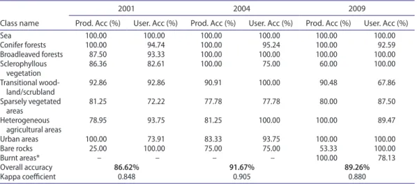
From the SVMs classification implementation, three classified images were obtained showing a clear spatial heterogeneity among the different classes. The following 10 classes were extracted after the image classification Sea, Heterogeneous Agricultural Areas, Broadleaved forests, Bare rocks, Urban Areas, Sparsely Vegetated Areas, Burnt areas, Conifer forests, Sclerophyllous Vegetation and Transitional Woodland/Scrubland. A very high OA was reported for all three classification images (OA: 86.62% in 2001, 91.67% in 2004 and 89.26% for 2009). Kappa statistic was high in all images, with values of 0.848, 0.905 and 0.880 for 2001, 2004 and 2009, respectively (Table 3, Figure 3). Some lower accuracy in 2001 classified can be related to the acquisition dates of the images. Coniferous forest/Broadleaved forest can show different behaviour for example, dropping of leaves and spectral changes in leaf colour is rather related to the climate than the calendar date. For most of the classes, the PA of > 85% was obtained except for sparsely vegetated areas, heterogeneous agricultural areas and bare rocks which suggested that the collected validation samples also belonged to the same class more frequently. No burnt areas are detected in 2001 and 2004 images. Similarly, UA is found in the range of 80–100% for most of the classes indicated that all of the points classified by the SVMs could be expected to be the same area when a field survey is performed. The classification of the bare rocks and vegetated areas in different categories indicated a lower PA and UA most of the time than the other classes can be attributed to misclassification errors because of closed similarity of vegetation classes with each other.
These statistics are highly sufficient for making a robust analysis of the study area because they exceed the minimum 85% OA stipulated by the USGS classification scheme (Anderson et al. 1976) for satellite-derived LULC maps and also as was adopted in recent research studies (Deng et al. 2009; Singh et al. 2013a, 2013b, 2015; Srivastava et al. 2014). It can be observed that the upper parts of the Hyperion images were mostly covered by Heterogeneous Agricultural Areas and Urban Areas on the top north. The middle parts were dominated by three LULC classes including Conifer forests, Sclerophyllous Vegetation and Transitional Woodland/Scrubland. On the other hand, the parts towards the south were mainly covered by Urban Areas. The class ‘Burnt Areas’ was spotted only in the centre of 2009 image because the fire occurred after 2007 (Petropoulos, Arvanitis, et al., 2012). However, the
class ‘Bare Rocks’ was found close to the urban areas in the south of the study region and also in the centre of 2009 image after fire occurrence. Similar kind of LULC trends could be observed visually by analysing either the Hyperion imagery or observing a Google Earth imagery of the site within the same or near image acquisition period.
5.2. Quantifying land cover change
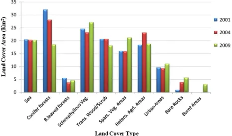
Different trends of change were found during the nine-year period covered by the three Hyperion images. In 2001, the computed area of each LULC class showed that Conifer forests, Sclerophyllous Vegetation and Transitional Woodland/Scrubland occupied the largest areas by 31.94, 24.48 and 20.63
Figure 3. land use/cover classification results from Hyperion time-series images 2001, 2004 and 2009 using the SVMs pixel-based classifier.
Table 3. classification accuracy of the three Hyperion scenes 2001, 2004 and 2009. Class name
2001 2004 2009
Prod. Acc (%) User. Acc (%) Prod. Acc (%) User. Acc (%) Prod. Acc (%) User. Acc (%)
Sea 100.00 100.00 100.00 100.00 100.00 100.00 conifer forests 100.00 94.74 100.00 95.24 100.00 92.59 Broadleaved forests 87.50 93.33 100.00 100.00 100.00 100.00 Sclerophyllous vegetation 86.36 82.61 100.00 75.00 60.00 100.00 transitional wood-land/scrubland 92.86 92.86 90.91 100.00 90.48 67.86 Sparsely vegetated areas 81.25 72.22 77.78 77.78 80.00 87.50 Heterogeneous agricultural areas 78.95 93.75 81.25 100.00 100.00 89.47 Urban areas 100.00 73.91 83.33 93.75 100.00 100.00 Bare rocks 25.00 100.00 75.00 75.00 53.33 100.00 Burnt areas* – – – – 100.00 78.13 overall accuracy 86.62% 91.67% 89.26% Kappa coefficient 0.848 0.905 0.880
Km2, respectively, while Sparsely Vegetated Areas and Heterogeneous Agricultural Areas arrived in
the second rank by 16.02 and 18.39 Km2, respectively, in the third rank we found Broadleaved forests
by 5.48 Km2 and Urban Areas by 9.51 Km2, and finally the class Bare Rocks with only 0.87 Km2. In
2004, the intra-changes of LULC statistics were close to 2001 somehow and following the same trend of changes. Comparing to 2001, a decrease in LULC surface was registered for five classes including Conifer forests, Broadleaved forests, Sclerophyllous Vegetation, Sparsely Vegetated Areas and Urban Areas. On the other side, a big increase of LULC surface was registered for Heterogeneous Agricultural Areas and Bare Rocks, for Transitional Woodland/Scrubland almost the same area was registered. In 2009, comparing to 2004 some LULC classes continued their decrease, which was the case for Conifer forests, Transitional Woodland/Scrubland and Heterogeneous Agricultural Areas, whereas
Figure 4. land cover type proportions for each of the three dates; 2001, 2004 and 2009.
Figure 5. Scatterplot of ordination results gained with landscape metrics ( : 2001; ●: 2004; : 2009; —: change trajectories of land cover types; c: coniferous forest; H: heterogeneous agricultural areas; Ba: bare rocks; Br: broadleaved forests; U: urban areas; Sc: sclerophyllous vegetation; t: transitional woodland/scrubland).
some of them showed a recovery and an increase was registered for Broadleaved forests, Sclerophyllous Vegetation, Sparsely Vegetated Areas, Urban Areas and Bare Rocks, a new class was created in 2009 image represented by Burnt Areas which was found in the centre of the study region after the fire of 2007 (Table 4, Figure 4).
Results also suggested a high rate of deforestation in the centre of the region as well as a high rate of urbanization in northern and southern parts (Table 5); possibly due to large demand of natural resources for different industrial activities. Furthermore, the fast increase in Bare Rocks LULC class in the middle part of the region was resulted from the land clearing following the fire of 2007. Apart from disaster like forest fire, the other reasons for land use/land cover changes are unprecedented rise in human population and non-judicious utilization of vegetated area by local people for resources like fuel wood, timber, non-timber forest products and fodder.
5.3. Landscape metrics using FRAGSTATS®
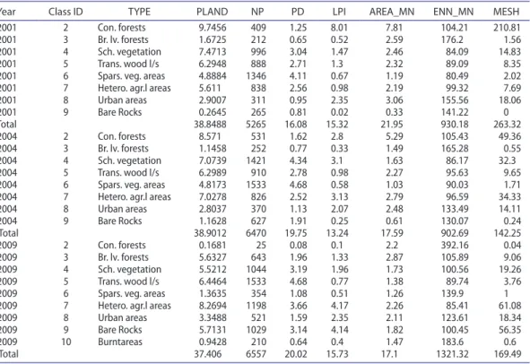
LULC analysis results showed that Sclerophyllous Veg. is a dominant land cover type in 2009. The landscape class level metrics results are shown in Table 6. The maximum Percentage of Landscape (PLAND) in 2001 shown by conifer forests (9.74%) and minimum by bare rocks (0.26%), in 2004 again conifer forests have maximum PLAND (8.57) and minimum broad leaved forests (1.14), whereas in 2009 maximum PLAND was reported for heterogeneous agricultural areas (8.26) and minimum (0.16) for conifer forests (Table 6). The result of PLAND shows that the Conifer forests are dominant in the region and overall trend showed it is decreasing; in year 2009 as dominant cover type was sparsely vegetated areas. The NP was highest for the sparsely vegetated areas (1346) and minimum for broad leaved forests (212) in 2001, this suggests that the sparsely vegetated areas are more frag-mented towards disturbances across a landscape whereas broad leaved forests are more resistant to disturbances. In 2004, again the sparsely vegetated areas have maximum NP (1533) and minimum
Table 4. total amount of each land cover class in the site (Km2).
Land cover type 2001 2004 2009
Sea 20.24 20.23 20.22
conifer forests 31.94 28.09 18.46
Broadleaved forests 5.48 3.75 4.47
Sclerophyllous Veg. 24.48 23.18 27.1
trans. wood/scrub 20.63 20.64 18.09
Spars. veg. areas 16.02 15.79 21.13
Hetero. agri. areas 18.39 23.03 18.72
Urban areas 9.51 9.19 10.98
Bare rocks 0.87 3.81 5.56
Burnt areas 0 0 3.09
Table 5. land Use/cover changes from 2001 to 2009 (Km2) according to the SVMs classifier implementation to the Hyperion images. Land cover type
Land cover area (Km2)
2001–2004 2004–2009 2001–2009 Sea −0.17 −0.11 −0.28 conifer forests −3.85 −9.63 −13.48 B.leaved forests −1.73 0.71 −1.01 Sclerophyllous veg. −1.3 3.92 2.62 trans. wood/scrub 0.01 −2.55 −2.54
Spars. veg. areas −0.23 5.34 5.11
Hetero. agri. areas 4.64 −4.31 0.33
Urban areas −0.32 1.79 1.47
Bare rocks 2.94 1.74 4.69
was reported for broad leaved forests. In 2009, the highest NP (1533) was obtained for transitional woodland/scrubland and minimum NP (25) was for conifer forests. It means that the conifer forests are very less resistant towards disturbances like forest fire. The changes in the patch density (PD) or mean patch size (MPS) at landscape level is defined by PD/MPS revealed that the sparsely vegetated areas get the highest patch density (4.11 Nber/100 ha), whereas broadleaf forests has lowest PD (0.65 Nber/100 ha) in 2001. The PD was highest for sparsely vegetated areas (4.68 Nber/100 ha) whereas the broad leaf forests demonstrate the lowest PD (0.77 Nber/100 ha) in 2004. PD was the highest for the transitional woodland/scrubland (4.68 Nber/100 ha) and was the lowest in the case of conifer forests (0.08 Nber/100 ha). It suggested that the conifer forest was more fragmented in 2009 as correlated to previous years. The largest patch index at the class level computes the percentage of total landscape area involved inside the largest patch. Independently, it is a straightforward estimate for dominance. The maximum of LPI was obtained for the conifer forests (8.01%) and the minimum of (0.02%) for bare rocks in 2001. In 2004, the maximum LPI was observed for heterogeneous agricultural areas (3.13%) and minimum (0.25%) for bare rocks, whereas in 2009, the maximum LPI was observed for heterogeneous agricultural areas (4.17%) and minimum for burnt areas (0.4%). It has been suggested that the heterogeneous agricultural areas are getting dominated in the region over the period. 5.4. Trend of fragmentation by LU/LC classes
The multivariate analysis (i.e. the PCA) provided a possibility to analyse the data-set considering several landscape metrics parallel (Huang et al. 2008; Szabó et al. 2015). This approach made possible to identify trends in the changes from the aspect of landscape fragmentation. The involved landscape metrics resulted in a good fit according to the RMSR and GFI (0.06 and 0.99, respectively). PCA explained 89.1% of the total variance (Table 7). PC1 accounted for the 45.6% of the variance correlating
Table 6. FraGStatS® metrics of lU/lc classes during 2001, 2004 and 2009 (area/density/edge metrics) of class and landscape metrics (_Mn: arithmetic mean of patch level data).
Year Class ID TYPE PLAND NP PD LPI AREA_MN ENN_MN MESH
2001 2 con. forests 9.7456 409 1.25 8.01 7.81 104.21 210.81
2001 3 Br. lv. forests 1.6725 212 0.65 0.52 2.59 176.2 1.56
2001 4 Sch. vegetation 7.4713 996 3.04 1.47 2.46 84.09 14.83
2001 5 trans. wood l/s 6.2948 888 2.71 1.3 2.32 89.09 8.35
2001 6 Spars. veg. areas 4.8884 1346 4.11 0.67 1.19 80.49 2.02
2001 7 Hetero. agr.l areas 5.611 838 2.56 0.98 2.19 99.32 7.69
2001 8 Urban areas 2.9007 311 0.95 2.35 3.06 155.56 18.06 2001 9 Bare rocks 0.2645 265 0.81 0.02 0.33 141.22 0 total 38.8488 5265 16.08 15.32 21.95 930.18 263.32 2004 2 con. forests 8.571 531 1.62 2.8 5.29 105.43 49.36 2004 3 Br. lv. forests 1.1458 252 0.77 0.33 1.49 165.28 0.55 2004 4 Sch. vegetation 7.0739 1421 4.34 3.1 1.63 86.17 32.3 2004 5 trans. wood l/s 6.2989 910 2.78 0.98 2.27 95.63 9.65
2004 6 Spars. veg. areas 4.8173 1533 4.68 0.58 1.03 90.03 1.71
2004 7 Hetero. agr.l areas 7.0278 826 2.52 3.13 2.79 96.59 34.33
2004 8 Urban areas 2.8037 370 1.13 2.07 2.48 133.49 14.11 2004 9 Bare rocks 1.1628 627 1.91 0.25 0.61 130.07 0.24 total 38.9012 6470 19.75 13.24 17.59 902.69 142.25 2009 2 con. forests 0.1681 25 0.08 0.1 2.2 392.16 0.04 2009 3 Br. lv. forests 5.6327 643 1.96 1.33 2.87 105.89 9.06 2009 4 Sch. vegetation 5.5212 1044 3.19 1.96 1.73 100.56 19.26 2009 5 trans. wood l/s 6.4464 1533 4.68 0.77 1.38 89.74 3.76
2009 6 Spars. veg. areas 1.3635 354 1.08 0.51 1.26 139.9 1
2009 7 Hetero. agr.l areas 8.2694 1198 3.66 4.17 2.26 85.41 61.08
2009 8 Urban areas 3.3488 521 1.59 2.35 2.11 123.61 18.34
2009 9 Bare rocks 5.7131 1029 3.14 4.14 1.82 100.45 56.35
2009 10 Burntareas 0.9428 210 0.64 0.4 1.47 183.6 0.6
with the MESH, LPI and AREA (as area-related metrics), while PC2 accounted for the 43.5% of the variance in high correlation with the NP, PD and ENN (as patch density and distance related metrics).
Changes were revealed based on PC1 and PC2 variables (Figure 5). Largest changes occurred in case of conifer forests as the trajectory of the dates can be considered large on both axis: magnitude of the changes was the largest decrease among all land cover types regarding both PCs. Changes of urban areas were the smallest. Trends were distinguished as monotonously decreasing (conifer forest) monotonously increasing (heterogeneous agricultural areas, bare rocks), transitional ones (changes were different along the two axis: broadleaved forests, urban areas, transitional woodland/scrubland) and when there was no trend (sclerophyllous vegetation).
Conifer forests have a decreasing trend. The effective mesh size (MESH), which is an indicator of subdivision characteristic of a landscape (Jaeger 2000), Largest Patch Index (LPI) and the mean area (AREA) decreased in the investigated period, number of patches (NP), patch density (PD) also decreased. Consequently, the mean distance of the nearest neighbouring patch (ENN) increased. This process indicates a fast fragmentation process that can be considered as the most detrimental process in the area as these forests play an important role in the sustaining of the biodiversity. Moreover, other natural habitats (sclerophyllous forests and sparsely vegetated areas) are also endangered by the head-way of bare rocks and agricultural lands. The slow increase in urban area patch sizes also indicates that the region will face the sprawl of the increasing rate of built-up areas enhancing the anthropogenic influence on the valuable species (Fahrig 1997).
6. Conclusions
This study aimed at exploring the use of Hyperion imagery synergistically with SVMs to map LULC change dynamics over a 9-year period (2001–2009) in a typical Mediterranean ecosystem and sub-sequently the relationships between LULC changes in landscape fragmentation characteristics. To our knowledge, this study is the first of its kind, in terms of providing the first demonstration of the Hyperion EO-1 capability combined with FRAGSTATS® in monitoring LULC changes and
under-standing land surface fragmentation characteristics and their changes over time.
Our findings unveil the degree of land use change, diversity and fragmentation patterns occurred, indicating that notable changes have taken place in the studied area during the 9 years. Landscape metric and landscape transformation analysis showed that over the time spatial configuration and composition of the landscape has significantly changed as a result of both natural hazards and anthro-pogenic activities pressures, resulting to a reduction in the forest area. These results overall suggested the requirement for using the most convenient approaches to conserve this precious ecologically natural ecosystem of the region.
Our study findings provide an important input to the understanding of the landscape metrics of complex and highly dynamic ecosystems in the Mediterranean region. More importantly, provide further supporting evidence of the suitability of synergistic use of EO with GIS in monitoring the variations within landscape dynamics in a cost-effective, semi-automatic and rapid manner. Notably, the approach implemented here in particular is robust and adjustable enough to be expanded further or to be implemented to other regions as well after necessary adjustments are made. The latter is of
Table 7. rotated component matrix of the selected landscape metrics.
FRAGSTATS® metrics PC1 PC2
effective mesh size (MeSH) 0.971 0.040
largest patch index (lPI) 0.948 0.172
Patch area (area) 0.912 −0.197
number of patches (nP) −0.100 0.970
Patch density (PD) −0.100 0.970
euclidean nearest neighbour distance (enn) −0.217 −0.814
considerable importance given the booming access to freely distributed EO data globally and par-ticularly the forthcoming launch of new satellite-based hyperspectral sensors just as that of NASA’s HyspIRI and EnMAP, the German hyperspectral satellite mission to be launched in 2018.
Acknowledgements
Authors wish to thank the United States Geological Survey (USGS) for the free access to the satellite data used in the present study. Finally, authors are grateful to the anonymous reviewers for their comments which assisted in improving the manuscript.
Disclosure statement
No potential conflict of interest was reported by the authors. ORCID
Salim Lamine http://orcid.org/0000-0002-0183-8820
George P. Petropoulos http://orcid.org/0000-0003-1442-1423
References
Anderson JRHE, Roach JT, Witmer RE. 1976. A land use and land cover classification system for use with remote sensor data. Washington, DC: USG Survey.
Basto M, Pereira JM. 2012. An SPSS R – menu for ordinal factor analysis. J Statist Software. 46. doi: http://dx.doi. org/http://dx.doi.org/10.18637/jss.v046.i04.
Bazi Y, Melgani F. 2006. Toward an optimal SVM classification system for hyperspectral remote sensing images. IEEE Trans Geosci Remote Sens. 44:3374–3385, November.
Beck R. 2003. EO-1 User Guide v. 2.3. Sioux Falls: Department of Geography University of Cincinnati.
Bissonette JA. 2008. Habitat fragmentation and landscape change: an ecological and conservation synthesis David B. Lindenmayer and Joern Fischer. 2006. Washington, DC: Island Press. Cloth $80.00, ISBN: 1-59726-020-7. Paper, $39.95. ISBN:1-59726-021-5. 352 pages. Ecological Restoration. 2008/05/13;26:162–164.
Bonan GB, Levis S, Kergoat L, Oleson KW. 2002. Landscapes as patches of plant functional types: an integrating concept for climate and ecosystem models. Global Biogeochem Cycles. May 22;16:5-1-5-23.
Borak JS. 1999. Feature selection and land cover classification of a MODIS-like data set for a semiarid environment. Int J Remote Sens. Jan;20:919–938.
Burges C. 1998. A tutorial on support vector machines for pattern recognition. Data Min Knowl Discov. 2:121–167. Çakir G, Sivrikaya F, Keleş S. 2007. Forest cover change and fragmentation using Landsat data in Maçka State Forest
Enterprise in Turkey. Environ Monit Assess. May 23;137:51–66.
Congalton R, Green K. 1998. Assessing the accuracy of remotely sensed data. In: Mapping science. CRC Press; p. 2154–7181. doi: http://dx.doi.org/http://dx.doi.org/10.1201/9781420048568.
Deng JS, Wang K, Hong Y, Qi JG. 2009. Spatio-temporal dynamics and evolution of land use change and landscape pattern in response to rapid urbanization. Landscape Urban Plann. Sep;92:187–198.
Elatawneh A, Kalaitzidis C, Petropoulos GP, Schneider T. 2014. Evaluation of diverse classification approaches for land use/cover mapping in a Mediterranean region utilizing Hyperion data. Int J Digital Earth. 7:194–216. doi: http:// dx.doi.org/10.1080/17538947.2012.671378.
Elkie PC, Rempel RS, Carr AP. 1999. Patch analyst user’s manual: a tool for quantifying landscape structure. Ontario, Canada.
ENVI. 2008. ENVI user’s manual. Boulder (CO): ITT Visual Information Solutions.
Fahrig L. 1997. Relative effects of habitat loss and fragmentation on population extinction. J Wildlife Manage. Jul;61:603– 610. doi: http://dx.doi.org/http://dx.doi.org/10.2307/3802168.
Fauvel M, Chanussot J, Benediktsson JA. 2006. Evaluation of kernels for multiclass classification of hyperspectral remote sensing data. Proceedings of the 2006 IEEE International Conference on Acoustics Speech and Signal Processing Proceedings; 2006 14–19 May 2006.
Foody GM, Mathur A. 2004. A relative evaluation of multiclass image classification by support vector machines. IEEE Trans Geosci Remote Sens. Jun;42:1335–1343.
Galvão LS, Formaggio AR, Tisot DA. 2005. Discrimination of sugarcane varieties in Southeastern Brazil with EO-1 Hyperion data. Remote Sens Environ. Feb;94:523–534.
Herold M, Liu X, Clarke KC. 2003. Spatial metrics and image texture for mapping urban land use. Photogrammet Eng Remote Sens. Sep 1;69:991–1001.
Huang C, Song K, Kim S, Townshend JRG, Davis P, Masek JG, Goward SN. 2008. Use of a dark object concept and support vector machines to automate forest cover change analysis. Remote Sens Environ. Mar;112:970–985. Jaeger JAG. 2000. Landscape division, splitting index, and effective mesh size: new measures of landscape fragmentation.
Landscape Ecol. 15:115–130.
Jolliffe IT. 1986. Principal component analysis and factor analysis. In: Principal component analysis. New York (NY): Springer Science + Business Media; p. 115–128.
JRC-EEA. 2005. CORINE land cover updating for the year 2000. Image 2000 and CLC 2000. In: Lima V, editor. Products and methods (Report EUR 21757 EN). JRCIspra.
Kamusoko C, Aniya M. 2007. Land use/cover change and landscape fragmentation analysis in the Bindura District, Zimbabwe. Land Degrad Dev. 18:221–233.
Karamesouti M, Petropoulos GP, Papanikolaou ID, Kairis O, Kosmas K. 2016. Erosion rate predictions from PESERA and RUSLE at a Mediterranean site before and after a wildfire: comparison & implications. Geoderma. Jan;261:44–58. Kuemmerle T, Chaskovskyy O, Knorn J, Radeloff VC, Kruhlov I, Keeton WS, Hostert P. 2009. Forest cover change and
illegal logging in the Ukrainian Carpathians in the transition period from 1988 to 2007. Remote Sens Environ. Jun 15;113:1194–1207.
Lamine S, Petropoulos GP. 2013. Evaluation of the spectral angle mapper “SAM” classification technique using hyperion imagery. Proceedings of the European Space Agency Living Planet Symposium; 2013 September; UK: The University of Nottingham.
Latifovic R, Fytas K, Chen J, Paraszczak J. 2005. Assessing land cover change resulting from large surface mining development. Int J Appl Earth Observ Geoinf. May;7:29–48.
Li D-C, Liu C-W. 2010. A class possibility based kernel to increase classification accuracy for small data sets using support vector machines. Expert Syst Appl. Apr;37:3104–3110.
Li S, Kwok JTY, Tsang IWH, Wang Y. 2004. Fusing images with different focuses using support vector machines. IEEE Trans Neural Netw. Nov;15:1555–1561.
Lu D, Weng Q. 2007. A survey of image classification methods and techniques for improving classification performance. Int J Remote Sens. Mar;28:823–870.
Lu L, Li X, Cheng G. 2003. Landscape evolution in the middle Heihe River Basin of north-west China during the last decade. J Arid Environ. Mar;53:395–408.
Luo Y, Liao M, Yan J, Zhang C. 2012. A multi-features fusion support vector machine method (MF-SVM) for classification of mangrove remote sensing image. J Computat Inf Syst. 8:323–334.
MacLean MG, Congalton RG. 2015. A comparison of landscape fragmentation analysis programs for identifying possible invasive plant species locations in forest edge. Landscape Ecol. Feb 20;30:1241–1256.
McGarigal K, Cushman S, Ene E. 2012. FRAGSTATS v4: spatial pattern analysis program for categorical and continuous maps. Amherst: University of Massachusetts.
Mathur A, Foody GM. 2008. Crop classification by support vector machine with intelligently selected training data for an operational application. Int J Remote Sens. Apr;29:2227–2240.
Otukei JR, Blaschke T. 2010. Land cover change assessment using decision trees, support vector machines and maximum likelihood classification algorithms. Int J Appl Earth Observ Geoinf. Feb;12:S27–S31.
Pal M, Mather PM. 2006. Some issues in the classification of DAIS hyperspectral data. Int J Remote Sens. Jul 20;27:2895– 2916.
Pengra BW, Johnston CA, Loveland TR. 2007. Mapping an invasive plant, Phragmites australis, in coastal wetlands using the EO-1 Hyperion hyperspectral sensor. Remote Sens Environ. May;108:74–81.
Petropoulos GP, Knorr W, Scholze M, Boschetti L, Karantounias G. 2010. Combining ASTER multispectral imagery analysis and support vector machines for rapid and cost-effective post-fire assessment: a case study from the Greek wildland fires of 2007. Natural Hazards Earth Syst Sci. 10:305–317.
Petropoulos GP, Kontoes C, Keramitsoglou I. 2011. Burnt area delineation from a uni-temporal perspective based on Landsat TM imagery classification using support vector machines. Int J Appl Earth Observ Geoinf. Feb;13:70–80. Petropoulos GP, Kalaitzidis C, Prasad Vadrevu K. 2012. Support vector machines and object-based classification for
obtaining land-use/cover cartography from Hyperion hyperspectral imagery. Comput Geosci. Apr;41:99–107. Petropoulos GP, Arvanitis K, Sigrimis N. 2012. Hyperion hyperspectral imagery analysis combined with machine
learning classifiers for land use/cover mapping. Expert Syst Appl. 39:3800–3809.
Petropoulos GP, Partsinevelos P, Mitraka Z. 2013. Change detection of surface mining activity and reclamation based on a machine learning approach of multi-temporal Landsat TM imagery. Geocarto Int. 28:323–342. doi:http://dx.doi. org/10.1080/10106049.2012.706648.
Petropoulos GP, Vadrevu KP, Kalaitzidis C. 2013. Spectral angle mapper and object-based classification combined with hyperspectral remote sensing imagery for obtaining land use/cover mapping in a Mediterranean region. Geocarto Int. Apr;28:114–129.
Petropoulos GP, Manevski K, Carlson TN. 2014. Hyperspectral remote sensing with emphasis on land cover mapping: from ground to satellite observations. In: Weng Q, editor. Scale issues in remote sensing. Hoboken (NJ): Wiley-Blackwell; p. 285–320. doi:http://dx.doi.org/10.1002/9781118801628.ch15.
Petropoulos GP, Kalivas DP, Georgopoulou H, Srivastava PK. 2015. Urban vegetation cover extraction from hyperspectral remote sensing imagery & GIS spatial analysis techniques: the case of Athens, Greece. J Appl Remote Sens. 9:1–18. 0091-3286/2015.
Pignatti S, Cavalli RM, Cuomo V, Fusilli L, Pascucci S, Poscolieri M, Santini F. 2009. Evaluating Hyperion capability for land cover mapping in a fragmented ecosystem: Pollino National Park, Italy. Remote Sens of Environ. Mar;113:622– 634.
Raines GL. 2002. Description and comparison of geologic maps with FRAGSTATS – a spatial statistics program. Comput Geosci. Mar;28:169–177.
Ricketts TH. 2001. The matrix matters: effective isolation in fragmented landscapes. Am Nat. Jul;158:87–99.
Saumitra M, Satyanarayan S, Gupta M, Manoj KP, Chandar S, Sudhir KS, Srivastava PK, Kamalesh KS. 2007. Integrated water resource management using remote sensing and geophysical techniques: aravali quartzite, Delhi, India. J Environ hydrol. 15: 1–10.
Sawaya KE, Olmanson LG, Heinert NJ, Brezonik PL, Bauer ME. 2003. Extending satellite remote sensing to local scales: land and water resource monitoring using high-resolution imagery. Remote Sens Environ. Nov;88:144–156. Singh SK, Srivastava PK, Pandey AC, Gautam SK. 2013a. Integrated assessment of groundwater influenced by a confluence
river system: concurrence with remote sensing and geochemical modelling. Water Resour Manage. Jul 7;27:4291–4313. Singh SK, Srivastava PK, Gupta M, Thakur JK, Mukherjee S. 2013b. Appraisal of land use/land cover of mangrove forest
ecosystem using support vector machine. Environ Earth Sci. Nov 8;71:2245–2255.
Singh SK, Mustak S, Srivastava PK, Szabó S, Islam T. 2015. Predicting spatial and decadal LULC changes through cellular automata markov chain models using earth observation datasets and geo-information. Environ Process. doi: http:// dx.doi.org/10.1007/s40710-015-0062-x.
Singh SK, Srivastava PK, Szabó S, Petropoulos GP, Gupta M, Islam T. 2016. Landscape transform and spatial metrics for mapping spatiotemporal land cover dynamics using Earth Observation data-sets. Geocarto Int. Jan 25;58:1–15. Srivastava PK, Han D, Rico-Ramirez MA, Bray M, Islam T. 2012. Selection of classification techniques for land use/land
cover change investigation. Adv Space Res. Nov;50:1250–1265.
Srivastava PK, Mukherjee S, Gupta M, Islam T. 2014. Remote sensing applications in environmental research. In: Springer, editor. Switzerland: Springer International Publishing. doi:http://dx.doi.org/10.1007/978-3-319-05906-8.
Szabó S, Bertalan L, Kerekes Á, Novák TJ. 2015. Possibilities of land use change analysis in a mountainous rural area: a methodological approach. Int J Geograph Inf Sci. 30:1–19.
Szilassi P, Jordan G, van Rompaey A, Csillag G. 2006. Impacts of historical land use changes on erosion and agricultural soil properties in the Kali Basin at Lake Balaton, Hungary. CATENA. 68:96–108.
Turner M. 1989. Landscape ecology: the effect of pattern on process. Ann Rev Ecol Syst. Jan 1;20:171–197. USGS. 2003. EO-1 user guide v. 2.3. Sioux Falls, SD: USGS-EROS. Available from: https://eo1.usgs.gov/documents/.
USGS. 2006. Hyperion level 1gst (L1GST) product output files data format control book (DFCB). Sioux Falls, SD 57198-0001.
Vapnik VN. 1998. Statistical learning theory. New York (NY): Wiley.
Volpi M, Petropoulo GP, Kanevski M. 2013. Flooding extent cartography with Landsat TM imagery and regularized kernel Fisher’s discriminant analysis. Comput Geosci. 57:24–31. doi:http://dx.doi.org/10.1016/j.cageo.2013.03.009. Waldhardt R, Simmering D, Otte A. 2004. Estimation and prediction of plant species richness in a mosaic landscape.
Landscape Ecol. 19:211–226.
Yuan J, Niu Z. 2007. Classification using EO-1 hyperion hyperspectral and ETM data. Fourth International Conference on Fuzzy Systems and Knowledge Discovery (FSKD 2007). Institute of Electrical & Electronics Engineers (IEEE). doi:http://dx.doi.org/10.1109/fskd.2007.218.
Zhang L, Huang X. 2010. Object-oriented subspace analysis for airborne hyperspectral remote sensing imagery. Neurocomputing. 73:927–936.