Statistical confidence intervals for relative abundances and
abundance-based ratios: simple practical solutions for an old
overlooked question
Baptiste Suchéras-Marx1 *, Gilles Escarguel2 *, Jorge Ferreira3, Øyvind Hammer4 1 Aix Marseille Univ, CNRS, IRD, INRA, Coll France, CEREGE, Aix-en-Provence, France 2 Université de Lyon, UMR 5023 LEHNA, UCBL, CNRS, ENTPE, F-69622 Villeurbanne, France 3 UMR CNRS 5276 LGL, Université Claude Bernard Lyon 1, Ecole Normale Supérieure Lyon, Campus de la Doua, 69622 Villeurbanne Cedex, France
4 Natural History Museum, University of Oslo, Pb. 1172, 0318 Oslo, Norway * Both authors contributed equally to this work
Abstract
Micropaleontologists often consider relative abundances of taxa to infer past ecological, environmental and climate conditions and dynamics. However, most published micropaleontological studies involving relative abundance data still do not routinely consider the counting uncertainty inherent to any sample, and thus simply ignore the statistical confidence interval (CI) related to a relative abundance or abundance-based ratio value. In an attempt to make this rather classic computation freely and easily available to the scientific community, we highlight here the calculation of binomial proportion CIs based on the ‘exact’ Clopper–Pearson method as implemented in the user-friendly PAST freeware. We also introduce a general solution for the computation of the CI related to any abundance-based ratio. In all cases, we strongly recommend that future studies involving taxonomic abundance-based data should systematically display the CIs associated to sample estimates, the only way to integrate sampling uncertainties into result interpretation.
1. Introduction
Micropaleontology is a diversified field within paleontology, focusing on different fossil groups from centimeter to micrometer-size and addressing a large array of scientific questions. It is commonly used in biostratigraphy, geochemistry, paleoecology, paleoclimatology and paleoenvironmental reconstructions, as well as evolutionary studies (e.g., Armstrong and Brasier, 2005; Saraswati and Srinivasan, 2016). Many works consider the relative abundances of taxa (expressed as proportions or percentages, based on counted fossil specimens per sample) as the starting point from which all subsequent analyses derive. Hence, many conclusive interpretations in micropaleontological studies are dependent upon the reliability of such relative abundance results.
Nannofossil micropaleontology (which focuses on the study of micrometer-sized calcareous platelets – coccoliths – produced by unicellular haptophyte algae and on calcite particles of incertae sedis organisms) provides numerous and diverse examples of relative abundance data-based studies. Such kind of data together with paleoclimatic interpretations have been abundantly produced over the last decades (e.g., McIntyre, 1967). This type of data is analysed from the Late Triassic – when these organisms first appear in the geological record (Gardin et al., 2012) – up to Holocene microfossil studies.
Among the micropaleontological studies dealing with relative abundances, only few works display the statistical CIs associated with empirical (i.e., sampled) proportions or percentages – e.g., pollens (Beaudoin et al., 2007); calcareous nannofossils (Beaufort et al., 2010; Suchéras-Marx et al., 2015); phytoliths (Strömberg and McInerney, 2011). This recurrent lack
of CIs undermines the statistical reliability of the interpretations and conclusions, a serious issue which has been often dealt with in the literature (e.g., Mosimann, 1965; Maher, 1981; Fatela and Taborda, 2002; Strömberg, 2009; Heslop et al., 2011), although so far with little practical application within the micropaleontological community.
In this note, we present a simple and rather classic practical solution on this issue, using the ‘exact’ Clopper–Pearson confidence interval method for relative abundance. Notwithstanding
some software being already available (e.g., PALYHELP
[http://www.ncdc.noaa.gov/paleo/softlib/palyhelp.html] or Dorai-Raj’s (2014) R Package 'binom' [https://cran.r-project.org/web/packages/binom/index.html]), such calculation is now implemented in the free and user-friendly statistical software PAST (Hammer et al., 2001). In addition, we introduce two solutions (in the form of an excel sheet and also implemented in PAST) for the computation of the CI related to any ratio contrasting the abundances of two or more taxa as customarily defined and used over the last decades in many paleoecological, paleoclimatic or paleoenvironmental micropaleontological studies. In order to increase the statistical reliability, we hope that such user-friendly computational solutions will encourage the micropaleontological community to provide the statistical confidence intervals associated with relative abundance and abundance-based ratio results.
2. Methods
2.1. The ‘exact’ Clopper–Pearson confidence interval for a relative abundance
Binomial proportion CI calculation in the case of asymptotic normal approximation (also called Wald CI) is the simplest way to calculate a binomial proportion CI; it was recommended by some previous authors (e.g., Fatela and Taborda, 2002). If p is the empirical (i.e., sampled) proportion and n the sample size, the 95% CI related to p is:
𝐶𝐼 = [𝑝 − 1.96√(𝑝(1−𝑝)
𝑛 ) ; 𝑝 + 1.96√( 𝑝(1−𝑝)
𝑛 )],
where 1.96 is the approximate value of the 97.5 percentile point of the standard Normal distribution.
The binomial proportion CI calculated with PAST since v. 3.06 is based on Clopper and Pearson’s (1934) method, which is a slightly more complex technique than Wald’s normal approximation. For = 0.05 (i.e., for a 1 – = 95% CI), x being the number of successes and n the number of trials, i.e., 𝑝 =𝑥
𝑛 is the empirical proportion of a taxon of interest (x
counted specimens) within a given sample made of n specimens, we have:
[1 + 𝑛−𝑥+1 𝑥𝐹[1−𝛼2;2𝑥,2(𝑛−𝑥+1)]] −1 < 𝑝 < [1 + 𝑛−𝑥+1 (𝑥+1)𝐹[𝛼2;2(𝑥+1),2(𝑛−𝑥)]] −1 ,
where F[c; d1, d2] denotes the 1 – c quantile of the Fisher distribution with d1 and d2 degrees
of freedom. The Clopper–Pearson method – referred as ‘exact’ since there is no approximation – outperforms the normal approximation methods for three main reasons: (i) it renders much more accurate confidence intervals for small-size samples; (ii) it cannot calculate CI boundaries beyond 0% and 100%; and (iii) it yields increasingly asymmetrical results as p departs from 50% whereas Wald CI is symmetric by definition.
Other proportion CI computation techniques exist (e.g., Brown et al., 2001). For instance,the Agresti-Coull, Wilson or Jeffreys CIs can be compared online to the Wald and
Clopper-Pearson CI using the EpiTools web page (http://epitools.ausvet.com.au/content.php?page=CIProportion). However, these three alternate (and computationally more complex) methods usually return CI boundaries very close to the Clopper–Pearson method, which is slightly more conservative in most cases – i.e., defining a slightly larger CI (Brown et al., 2001).
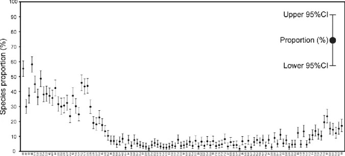
Figure 1: Representation of empirical (i.e., sampled) proportions (%) and associated binomial (Clopper–Pearson) 95% CIs in PAST v. 3.06 and higher (data: Biscutum constans from the Rødryggen section dataset published by Pauly et al., 2012).
2.2. Calculation procedure for a proportion CI using PAST v. 3.06 and higher
The free statistical software PAST (Hammer et al., 2001; https://folk.uio.no/ohammer/past/) is a steadily evolving and updated software for scientific data analysis. The latest released version is PAST 3.23 (February 2019) and the first version proposing computation of Clopper–Pearson 95% CI was PAST 3.06. The procedure for calculation is very simple and straightforward – see the 'Reference manual' provided by Ø. Hammer and updated every new version (http://folk.uio.no/ohammer/past/past3manual.pdf). Input data should be presented as following (see also Supplementary Fig. 1 and Supplementary Material 1):
- Rows: each row corresponds to a sample;
- Columns: except for the last one, each column corresponds to the empirical (i.e., sampled) percentage of a given taxon (ranging from 0 to 100%);
- Last column corresponds to the total number of counted specimens per sample.
Even if several taxa (columns) can be recorded in a single sample ordered by taxon in a spreadsheet, Clopper–Pearson 95% CI for one or more samples must be calculated for each taxon separately by selecting only two columns: the taxon of interest and the total number of specimens counted per sample (Supplementary Fig. 1). Users have to select the module 'Multiple Proportion CIs' from the menu 'Univariate' (Supplementary Fig. 1). The output result is displayed in a plot where empirical proportions are represented by dots (connected or not) and their associated 95% CIs are represented by whiskers (‘Plot’ tab; Figure 1, Supplementary Fig. 2). Samples can be plotted horizontally from left to right or vertically from bottom to top (‘flip axes’ option). As usual with PAST, a ‘Graph settings’ window offers several options to customize graphic preferences (e.g., graphic window size, font, font size, symbol size, min-max values and labels of the two axes, etc.). The resulting graph can finally
be saved (various formats available: SVG, PDF, JPG, TIFF…) and/or copied and pasted as a bitmap image. Alternatively, users can display results in a five-column numerical table format (including sample name, empirical percentage value, 95% CI lower and upper limits, and total number of specimens per sample) which can be directly copied and pasted in any text editor or spreadsheet program of their choice (‘Numbers’ tab; Supplementary Figs. 3, Supplementary Material 2).
2.3. Confidence intervals for taxonomic abundance-based ratios
Over the last two decades, numerous paleoenvironmental indices have been proposed in the micropaleontological literature, corresponding to abundance ratios of selected taxa (e.g., Aguado et al., 2014; Aizawa et al., 2004; Bornemann et al., 2005; Flores et al., 2000; Gale et al., 2000; Herrle, 2003, Herrle et al., 2003; Linnert et al., 2011; Marino et al., 2009; Mutterlose et al., 2014; Tiraboschi et al., 2009; Tremolada et al., 2006; Villa et al., 2008; Watkins and Self-Trail, 2005; see Supplementary Material 3). Such indices were based on the estimated ecological preferences of different taxa of interest. Even if they correspond to different taxon associations, all these paleoenvironmental indices can be expressed in a single general formula including three categories of taxa (see Supplementary Material 3):
- One or more taxa involved only in the numerator of the ratio; - One or more taxa involved only in the denominator of the ratio;
- One or more taxa involved simultaneously in the numerator and denominator of the ratio.
Whatever the actual number of taxa included in each category, let a, b, and c be the numbers of counted specimens (i.e., raw numbers of counted specimen) for each of these three categories, respectively; this gives the simple general form of the ratio 𝑟 =𝑎+𝑐
𝑏+𝑐. In some
cases, r involves all three categories of taxa (e.g., Herrle et al., 2003; Aguado et al., 2014); in this case, r ranges between 0 (when 𝑎 + 𝑐 = 0) and a + 1 (when b = 0 and c = 1), and is undefined (infinite) when 𝑏 + 𝑐 = 0. Alternatively, there can be no taxa shared by the numerator and denominator (i.e., c = 0), leading to 𝑟 =𝑎
𝑏 (e.g., Gale et al., 2000; Linnert et
al., 2011); in this case, r ranges between 0 (when a = 0) and a (when b = 1), and is undefined (infinite) when b =0. In most paleoenvironmental indices proposed so far, no taxa are involved only in the numerator (i.e., a = 0), giving 𝑟 = 𝑐
𝑏+𝑐 (see examples in
Supplementary Material 3). In this case, r ranges between 0 (when c = 0) and 1 (when b = 0), and can be expressed either as a proportion or a percentage (100).
Excluding the trivial case where 𝑏 + 𝑐 = 0, making 𝑟 = ∞, and considering the non-trivial situation where the numerator is non-zero, and thus r > 0, the statistical confidence interval of r results from the propagation of the binomial errors related to each sampled taxon, and thus related to a, b and c with respect to 𝑇 = 𝑎 + 𝑏 + 𝑐. In the particular (but most frequent) case where =𝑏+𝑐𝑐 , its CI is actually the binomial CI related to 𝑝 =𝑛𝑐 where 𝑛 = 𝑏 + 𝑐, making it possible to use the Clopper–Pearson method as detailed above and implemented in PAST v. 3.06 and higher. In all other cases (including 𝑟 =𝑎+𝑐
𝑏+𝑐, 𝑟 = 𝑎
𝑏, and also 𝑟 = 𝑎+𝑐
𝑐 ), r is not a
proportion and the analytical combination of such asymmetric and dependent errors is not straightforward (Barlow, 2004). Here we propose two solutions, one based on a Monte-Carlo procedure and using normal approximation of arcsine-transformed proportions and a second one based on a bootstrapping procedure.
For the Monte Carlo procedure, we first note that 𝑟 =𝑎+𝑐 𝑏+𝑐= 𝑎+𝑐 𝑇 𝑏+𝑐 𝑇 =( 𝑎 𝑇)+( 𝑐 𝑇) (𝑏𝑇)+(𝑇𝑐) where 𝑇 = 𝑎 + 𝑏 + 𝑐. Let e and g be the arcsine-transformed values related to the empirical proportions a/T and c/T, respectively, i.e.: 𝑒 = 𝑠𝑖𝑛−1(√𝑎
𝑇) and 𝑔 = 𝑠𝑖𝑛 −1(√𝑐
𝑇). By definition, e and g are normally
distributed variables with a sample standard deviation (s) of √1 (4𝑇)⁄ (Sokal and Rohlf, 2011). Let e* and g* be normally distributed random variates with mean e and g, and standard deviation s, respectively. Then, e* and g* are back-transformed to proportion values
(𝑎 𝑇) ∗ and (𝑐 𝑇) ∗ , i.e.: (𝑎 𝑇) ∗ = (𝑠𝑖𝑛(𝑒∗))2 and (𝑐 𝑇) ∗
= (𝑠𝑖𝑛(𝑔∗))2. Finally, a Monte-Carlo estimate
of r is calculated as 𝑟∗=( 𝑎 𝑇) ∗ +(𝑇𝑐)∗ 1−(𝑎𝑇)∗ – since 𝑇 = 𝑎 + 𝑏 + 𝑐, we have 𝑎 𝑇+ 𝑏 𝑇+ 𝑐 𝑇= 1, and thus 𝑏 𝑇+ 𝑐 𝑇 = 1 − 𝑎
𝑇, making the Monte-Carlo estimate of ( 𝑏 𝑇)
∗
unnecessary. This procedure is reiterated a large number of times (say, 10,000 times), ultimately leading to a Monte-Carlo distribution of the statistical uncertainty related to r, from which the 100−𝑥
2 and 100+𝑥
2 percentiles define the
lower and upper limits of the x% CI, respectively (e.g., the 2.5 and 97.5 percentiles for the 95% CI). We provide an Excel sheet designed to calculate the 90%, 95% and 99% CIs associated to r, Log10(r), and √𝑟 (Supplementary Material 5). This method is also available in PAST since v. 3.23.
Alternatively, confidence intervals for r can be estimated by bootstrapping (e.g., Davison and Hinkley, 1997). Random replicates of size T are constructed by resampling from the original sample with replacement. In practice this is done by selecting random a’, b’ and c’ with probabilities proportional to a, b and c (i.e., from a trinomial distribution, or binomial if one of a, b, c is zero). A large number (e.g., 10,000) of replicates are computed, and r’ is computed for each replicate. A 95% CI is then estimated from the distribution of r’. We have found that the confidence intervals estimated with bootstrapping and with the method described above generally converge for T>50, but for smaller sample sizes the bootstrapped CI is considerably smaller (Supplementary Material 6). Bootstrapped confidence intervals for r can be computed with PAST, v. 3.23 onwards.
3. Beyond counting strategy
Micropaleontologists use dedicated sample preparation techniques and counting procedures adapted to their goal (e.g., biostratigraphy, paleoecology, paleoclimatology) and to the different types of fossils under study. Since counting procedures are sampling procedures, all these techniques involve a minimum number of specimens to be recorded in order to achieve reliable results (e.g., Fatela and Taborda, 2002; Haidar et al., 2018). For instance, Fatela and Taborda (2002) suggested that a minimum of n = 100 counted specimens is needed to sample species representing at least 5% of the original population. This easy-to-use conclusion has been highly cited so far (189 citations based on ScienceDirect and 283 citations based on Google Scholar in January 2019), although Fatela and Taborda’s (2002) main recommendation was “Generally, we suggest that percent abundance given in micropaleontological studies should include the binomial error estimate” (op. cit., p. 169), which was not followed by most of the studies citing them.
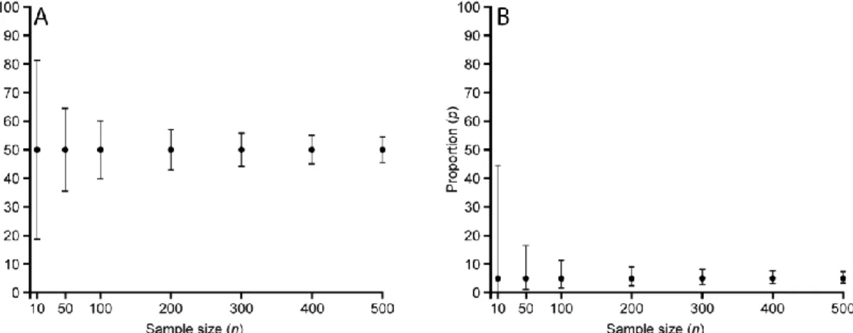
Indeed, the CI related to any empirical proportion p directly depends on p and n, as illustrated in Table 1 for some selected p-n couples as well as in Fig. 2 for p = 50% and p = 5%: for a given sample size (n), the CI increases as p becomes closer to 50%, whereas for a
given empirical proportion (p), the CI decreases as n increases – i.e., as the sampling effort increases, the empirical proportion p more and more accurately estimates the ‘real’ proportion value. n \ p 1% 5% 25% 50% 75% 95% 99% 10 [~0%; 30.9%] [0.25%; 44.5%] [2.52%; 55.6%] [18.7%; 81.3%] [44.4%; 97.5%] [55.5%; 99.7%] [69.2%; ~100%] 50 [~0%; 10.7%] [1.26%; 16.6%] [13.1%; 38.2%] [35.5%; 64.5%] [61.8%; 86.9%] [83.4%; 98.8%] [89.4%; ~100%] 100 [~0%; 5.45%] [1.64%; 11.3%] [16.9%; 34.7%] [39.8%; 60.2%] [65.3%; 83.1%] [88.7%; 98.4%] [94.6%; ~100%] 200 [0.12%; 3.57%] [2.42%; 9.00%] [19.2%; 31.6%] [42.9%; 57.1%] [68.4%; 80.8%] [91.0%; 97.6%] [96.4%; 99.9%] 300 [0.21%; 2.13%] [2.83%; 8.11%] [20.2%; 30.3%] [44.2%; 55.8%] [69.7%; 79.8%] [91.9%; 97.2%] [97.1%; 99.8%] 400 [0.27%; 2.54%] [3.08%; 7.62%] [20.8%; 29.5%] [45.0%; 55.0%] [70.5%; 79.2%] [92.4%; 96.9%] [97.5%; 99.7%] 500 [0.33%; 1.87%] [3.26%; 7.29%] [21.3%; 29.0%] [45.5%; 54.5%] [71.0%; 78.7%] [92.7%; 96.7%] [97.7%; 99.7%] Table 1: Clopper–Pearson 95% confidence intervals for selected p (sample proportion) and n (sample size = total number of counted specimens) values. Note that the CI is symmetric around p only for p = 50%, and becomes more and more asymmetric as p approaches 0% or 100%.
Figure 2: Effect of the empirical proportion p and sample size n values on the binomial (Clopper-Pearson) 95% CI (see Table 1 for detailed values). (A) p = 50%. (B) p = 5%.
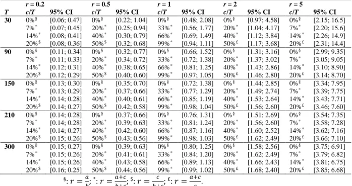
For the very same reason, it is exactly the same for a taxonomic abundance-based ratio, whose CI directly depends on the empirical ratio estimate r and sample size T, as well as on the relative number of specimens shared by the numerator and denominator of r (i.e., the c/T-value) (Table 2):
- For a given sample size (T), the CI increases as r increases; - For a given empirical ratio (r), the CI decreases as T increases; - For given T and r values, the CI decreases as c/T increases.
It is worth noting that the smallest CIs are expected for r values close to the unity and large c/T-values corresponding to a large percentage of counted specimens involved simultaneously in the numerator and denominator of r. This could naively argue against 𝑎𝑏 -type ratios and favor ratios where a large number of abundant taxa are shared by the numerator and denominator, leading to large c-values with respect to a and b. However, in this case, r variations from one sample to another are expected to be very small, strongly reducing the between-sample discrimination power of such ratio. From a purely statistical
point of view, a compromise must therefore be sought when defining a taxonomic abundance-based ratio by contrasting taxa with opposite characteristics at the numerator and denominator (increasing the between-sample discrimination power of r), and by also including taxa with ‘neutral’ characteristics shared by the numerator and denominator to control the extent of the CI.
r = 0.2 r = 0.5 r = 1 r = 2 r = 5 T c/T 95% CI c/T 95% CI c/T 95% CI c/T 95% CI c/T 95% CI 30 0%§ [0.06; 0.47] 0%§ [0.22; 1.04] 0%§ [0.48; 2.08] 0%§ [0.97; 4.58] 0%§ [2.15; 16.5] 7%* [0.07; 0.45] 20%* [0.25; 0.94] 33%* [0.56; 1.77] 20%* [1.04; 4.17] 7%* [2.20; 15.6] 14%* [0.08; 0.41] 40%* [0.30; 0.79] 66%* [0.69; 1.49] 40%* [1.12; 3.84] 14%* [2.26; 14.9] 20%$ [0.08; 0.36] 50%$ [0.32; 0.68] 99%* [0.94; 1.11] 50%£ [1.17; 3.68] 20%£ [2.31; 14.4] 90 0%§ [0.11; 0.34] 0%§ [0.32; 0.77] 0%§ [0.66; 1.52] 0%§ [1.31; 3.16] 0%§ [2.99; 9.35] 7%* [0.11; 0.33] 20%* [0.34; 0.72] 33%* [0.72; 1.38] 20%* [1.37; 3.02] 7%* [3.05; 9.05] 14%* [0.12; 0.31] 40%* [0.38; 0.65] 66%* [0.81; 1.25] 40%* [1.43; 2.86] 14%* [3.10; 8.90] 20%$ [0.12; 0.29] 50%$ [0.40; 0.60] 99%* [0.97; 1.05] 50%£ [1.46; 2.80] 20%£ [3.14; 8.70] 150 0%§ [0.13; 0.30] 0%§ [0.35; 0.70] 0%§ [0.72; 1.38] 0%§ [1.44; 2.85] 0%§ [3.34; 7.95] 7%* [0.13; 0.29] 20%* [0.37; 0.66] 33%* [0.77; 1.29] 20%* [1.49; 2.74] 7%* [3.39; 7.75] 14%* [0.14; 0.28] 40%* [0.40; 0.61] 66%* [0.85; 1.19] 40%* [1.53; 2.64] 14%* [3.43; 7.71] 20%$ [0.14; 0.27] 50%$ [0.42; 0.58] 99%* [0.98; 1.04] 50%£ [1.56; 2.60] 20%£ [3.46; 7.60] 210 0%§ [0.14; 0.28] 0%§ [0.37; 0.66] 0%§ [0.76; 1.31] 0%§ [1.51; 2.69] 0%§ [3.54; 7.35] 7%* [0.14; 0.28] 20%* [0.39; 0.63] 33%* [0.81; 1.24] 20%* [1.56; 2.60] 7%* [3.58; 7.28] 14%* [0.14; 0.27] 40%* [0.42; 0.60] 66%* [0.87; 1.16] 40%* [1.60; 2.52] 14%* [3.62; 7.16] 20%$ [0.15; 0.26] 50%$ [0.43; 0.56] 99%* [0.98; 1.03] 50%£ [1.62; 2.49] 20%£ [3.66; 7.10] 300 0%§ [0.15; 0.27] 0%§ [0.39; 0.63] 0%§ [0.80; 1.25] 0%§ [1.58; 2.56] 0%§ [3.75; 6.91] 7%* [0.15; 0.26] 20%* [0.41; 0.61] 33%* [0.84; 1.20] 20%* [1.62; 2.49] 7%* [3.79; 6.82] 14%* [0.15; 0.26] 40%* [0.43; 0.58] 66%* [0.89; 1.13] 40%* [1.66; 2.43] 14%* [3.81; 6.75] 20%$ [0.16; 0.25] 50%$ [0.44; 0.56] 99%* [0.99; 1.02] 50%£ [1.68; 2.40] 20%£ [3.85; 6.68] §: 𝑟 =𝑎 𝑏; *: 𝑟 = 𝑎+𝑐 𝑏+𝑐; $: 𝑟 = 𝑐 𝑏+𝑐; £: 𝑟 = 𝑎+𝑐 𝑐 .
Table 2: 95% confidence intervals for selected values of r (taxonomic abundance-based ratio), T (sample size = number of counted specimens participating in the computation of r), and c/T (percentage of counted specimens involved both in the numerator and denominator of r). Note that the CI converges towards [1; 1] as T and c/T increases and r becomes closer to 1.
4. Example: Rødryggen section from Pauly et al. (2012) published in Marine
Micropaleontology
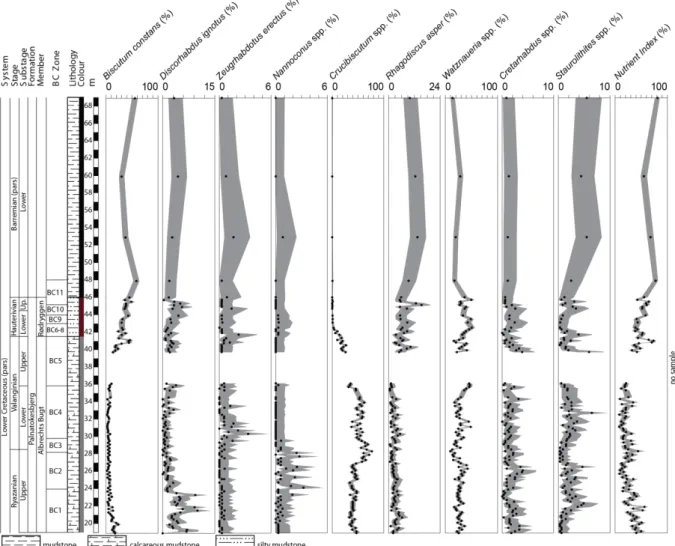
In order to highlight the benefits of CI computation, we have calculated the Clopper–Pearson 95% CI corresponding to Pauly et al.’s (2012) Rødryggen section dataset for nine coccolithophorid taxa of interest as well as for their Nutrient Index (Supplementary Material 4). These calculations are for illustrative purposes; we do not intend to discuss here Pauly et al.’s (2012) paleoenvironmental or paleoecological conclusions. Pauly et al. (2012) applied a common counting procedure by counting at least 300 specimens per sample. Figure 3 displays a plot similar to Pauly et al. (2012: fig. 3), but where the 95% CIs are added for each taxon as a gray interval, allowing for the direct observation of the statistical uncertainty related to each empirical relative abundance. For some taxa (e.g., Crucibiscutum spp.), there are indeed significant variations and long-term trends in relative abundance (i.e., percentage changes beyond the 95% CI of sample values). However, most of the variations recorded for less abundant taxa (e.g., Nannoconus spp. and Cretarhabdus spp.) fall within the 95% CI of the empirical percentages and therefore cannot be distinguished from random sampling noise of neither paleoenvironmental nor paleoecological significance. The 95% CI related to the Nutrient Index (NI; Pauly et al., 2012; Supplementary Material 3) also illustrates two contrasted situations (Fig. 3): in the Ryazanian to Lower Valanginian, a two-sample test between a single sample in the Ryazanian and a single sample in the Valanginian may
remain within the range of the 95% CI estimates; on the contrary, the increase between the Lower Valanginian and the Hauterivian–Barremian falls beyond the 95% CI, and therefore appears statistically consistent.
By illustrating examples of statistically significant and non-significant changes, this case study highlights the usefulness of calculating confidence intervals and integrating them into graphs representing variations of taxonomic relative abundances or abundance-based ratios. There is not, and there cannot be, any rule-of-thumb to avoid these calculations because the statistical significance of the difference between two samples is not only a matter of absolute difference between them, but also directly depends on the compared values as well as on the sample sizes. On one hand, with n = 300, a 10% absolute difference between 10% (95% CI: [6.85%; 14.0%]) and 20% (95% CI: [15.6%; 25.0%]) is significant, whereas another between 40% (95% CI: [34.4%; 45.8%]) and 50% (95% CI: [44.2%; 55.8%]) is not; on the other hand, a 15% absolute difference between 35% and 50% is significant for n = 200 (95% CI: [28.4%; 42.1%] vs. [42.9%; 57.1%]) whereas it is not for n = 100 (95% CI: [25.7%; 45.2%] vs. [39.8%; 60.2%]). Therefore CIs should always be made available by authors as they are the only actual way for both authors and readers to critically assess the statistical reliability of the analyzed data and results, as well as the proposed interpretations.
Figure 3: Pauly et al.’s (2012) fig. 3 with the 95% CIs for nine coccolithophorid taxa of interest and for the Nutrient Index (gray envelopes).
5. Conclusions
This study highlights the importance of calculating and graphically representing statistical confidence intervals related to taxonomic relative abundances and abundance-based ratios as customarily studied by micropaleontologists since several decades. For this purpose, easy-to-use computational solutions now exist, including the free and user-friendly PAST software which offers a module for calculating relative abundance CIs for one or more samples. In addition, we provide here an excel sheet and added in PAST two taxonomic abundance-based ratio CI calculation solutions. Since a statistical uncertainty necessarily results from any sampling procedure, a confidence interval should always be associated with any empirical proportion or ratio estimate to allow authors and readers to objectively describe, compare, interpret and discuss the meaning and implications of the sample data at hand. We hope that the scientific benefits combined with the easy access to practical and user-friendly computational solutions such as PAST will help and encourage micropaleontologists, reviewers and publishers to produce, require and ultimately publish statistical confidence intervals in future studies.
Acknowledgments
BSM thanks Fabienne Giraud and Emanuela Mattioli for support and discussions about the importance of confidence interval in micropaleontology; Luc Beaufort for discussions and references on the topic, Pierre Henry for his help, and Martin Tetard for comments on a previous version of the manuscript. This manuscript is a contribution to the team ‘Climat’ at
CEREGE (BSM).
Supplementary Materials
Suppl. Fig. 1 to 3: How to calculate binomial confidence intervals using PAST v. 3.06 and higher.
Suppl. Material 1: PAST input data example (.txt). Suppl. Material 2: PAST output data example (.txt).
Suppl. Material 3: Examples of Temperature and Fertility/Nutrient/Productivity indices published over the last two decades and their corresponding taxonomic abundance-based ratio type (.pdf).
Suppl. Material 4: Binomial Clopper–Pearson CIs calculated for the Rødryggen section dataset published by Pauly et al. (2012) (.csv).
Suppl. Material 5: Excel sheet for the calculation of confidence intervals (90%, 95% and 99% CIs) related to any taxonomic abundance-based ratio using Monte Carlo (.xlsx).
Suppl. Material 6: Comparison of Monte Carlo and bootstrapped confidence intervals for r, with a=b=c (r = 1) and for increasing sample sizes T = 3a (.csv).
References
Aguado, R., de Gea, G.A., Castro, J.M., O'Dogherty, L., Quijano, M.L., Naafs, B.D.A., Pancost, R.D., 2014. Late Barremian-early Aptian dark facies of the Subbetic (Betic Cordillera, southern Spain): Calcareous nannofossil quantitative analyses, chemostratigraphy and palaeoceanographic reconstructions. Palaeogeography, Palaeoclimatology, Palaeoecology 395, 198-221.
Aizawa, C., Oba, T., Okada, H., 2004. Late Quaternary paleoceanography deduced from coccolith assemblages in a piston core recovered off the central Japan coast. Marine Micropaleontology 52, 277-297.
Armstrong, H., Brasier, M.D., 2005. Microfossils, Second Edition. Blackwell Publishing, Oxford, UK, 296 pp.
Barlow, R., 2004. Asymmetric Statistical Errors. arXiv:physics/0406120.
Beaudouin, C., Jouet, G., Suc, J.-P., Berné, S., Escarguel, G., 2007. Vegetation dynamics in southern France during the last 30 ky BP in the light of marine palynology. Quaternary Science Reviews 26(7-8), 1037-1054.
Beaufort, L., van der Kaars, S., Moron, V., 2010. Past dynamics of the Australian monsoon: precession, phase and links to the global monsoon concept. Climate of the Past 6, 695-706.
Bornemann, A., Pross, J., Reichelt, K., Herrle, J.O., Hemleben, C., Mutterlose, J., 2005. Reconstruction of short-term palaeoceanographic changes during the formation of the Late Albian 'Niveau Breistroffer' black shales (Oceanic Anoxic Event 1d, SE France). Journal of the Geological Society 162, 623-639.
Brown, L.D., Cai, T.T., DasGupta, A., 2001. Interval estimation for a binomial proportion. Statistical Science 16, 101-117.
Clopper, C.J., Pearson, E.S., 1934. The use of confidence or fiducial limits illustrated in the case of the binomial. Biometrika 26, 404-413.
Davison, A.C., Hinkley, D.V., 1997. Bootstrap methods and their application. Cambridge University Press, 582 pp.
Dorai-Raj, S., 2014. Binomial confidence intervals for several parameterizations. R package 'binom'. 21 pp. http://cran.r-project.org/web/packages/binom/binom.pdf.
Fatela, F., Taborda, R., 2002. Confidence limits of species proportions in microfossil assemblages. Marine Micropaleontology 45(2), 169-174.
Flores, J.A., Bárcena, M.A., Sierro, F.J., 2000. Ocean-surface and wind dynamics in the Atlantic Ocean off Northwest Africa during the last 140 000 years. Palaeogeography, Palaeoclimatology, Palaeoecology 161, 459-478.
Gale, A.S., Smith, A.B., Monks, N.E.A., Young, J.A., Howard, A., Wray, D.S., Huggett, J.M., 2000. Marine biodiversity through the Late Cenomanian-Early Turonian: palaeoceanographic controls and sequence stratigraphic biases. Journal of the Geological Society 157, 745-757.
Gardin, S., Krystyn, L., Richoz, S., Bartolini, A., Galbrun, B., 2012. Where and when the earliest coccolithophores?. Lethaia 45(4), 507-523.
Haidar, A., Al-Hakim, A., Zhang, Z., 2018. Sample size for concurrent species detection in a species-rich assemblage. arXiv:1804.11226.
Hammer, Ø., Harper, D.A.T., Ryan, P.D., 2001. PAST: paleontological statistics software package for education and data analysis. Palaeontologia Electronica 4, 1-9.
Herrle, J.O., 2003. Reconstructing nutricline dynamics of mid-Cretaceous oceans: evidence from calcareous nannofossils from the Niveau Paquier black shale (SE France). Marine Micropaleontology 47, 307-321.
Herrle, J.O., Pross, J., Friedrich, O., Kössler, P., Hemleben, C., 2003. Forcing mechanisms for mid-Cretaceous black shale formation: evidence from the Upper Aptian and Lower Albian of the Vocontian Basin (SE France). Palaeogeography, Palaeoclimatology, Palaeoecology 190, 399-426.
Heslop, D., De Schepper, S., Proske, U., 2011. Diagnosing the uncertainty of taxa relative abundances derived from count data. Marine Micropaleontology 79(3-4), 114-120. Linnert, C., Mutterlose, J., Mortimore, R., 2011. Calcareous nannofossils from Eastbourne
(Southeastern England) and the paleoceanography of the Cenomanian-Turonian boundary interval. Palaios 26, 298-313.
Maher Jr, L.J., 1981. Statistics for microfossil concentration measurements employing samples spiked with marker grains. Review of Palaeobotany and Palynology 32(2-3), 153-191.
Marino, M., Maiorano, P., Lirer, F., Pelosi, N., 2009. Response of calcareous nannofossil assemblages to paleoenvironmental changes through the mid-Pleistocene revolution at Site 1090 (Southern Ocean). Palaeogeography, Palaeoclimatology, Palaeoecology 280, 333-349.
McIntyre, A., 1967. Coccoliths as paleoclimatic indicators of Pleistocene glaciation. Science 158, 1314-1317.
Mosimann, J.E., 1965. Statistical methods for the pollen analyst: multinomial and negative multinomial techniques. In: Kummel, B., Raup, D. (Eds.), Handbook of paleontological techniques. W.H. Freeman and Company, San Francisco, pp. 636-673.
Mutterlose, J., Bottini, C., Schouten, S., Sinninghe Damsté, J.S., 2014. High sea-surface temperatures during the early Aptian Oceanic Anoxic Event 1a in the Boreal Realm. Geology 42, 439-442.
Pauly, S., Mutterlose, J., Alsen, P., 2012. Early Cretaceous palaeoceanography of the Greenland-Norwegian Seaway evidenced by calcareous nannofossils. Marine Micropaleontology 90-91, 72-85.
Saraswati, P.K., Srinivasan, M.S., 2016. Micropaleontology. Springer, Heidelberg, 224 pp. Sokal, R.R., Rohlf, F.J., 2011. Biometry (4th Edition). W.H. Freeman & Co., New-York, 937
pp.
Strömberg, C.A.E., 2009. Methodological concerns for analysis of phytolith assemblages: Does count size matter? Quaternary International 193(1-2), 124-140.
Strömberg, C.A.E., McInerney, F.A., 2011. The Neogene transition from C3 to C4 grasslands in North America: assemblage analysis of fossil phytoliths. Paleobiology 37(1), 50-71. Suchéras-Marx, B., Giraud, F., Mattioli, E., Escarguel, G., 2015. Paleoenvironmental and
paleobiological origins of coccolithophorid genus Watznaueria emergence during the Late Aalenian-Early Bajocian. Paleobiology. DOI: 10.1017/pab.2015.8.
Tiraboschi, D., Erba, E., Jenkyns, H.C., 2009. Origin of rhythmic Albian black shales (Piobbico core, central Italy): Calcareous nannofossil quantitative and statistical analyses and paleoceanographic reconstructions. Paleoceanography 24, PA2222. Tremolada, F., Erba, E., Bralower, T.J., 2006. Late Barremian to early Aptian calcareous
nannofossil paleoceanography and paleoecology from the Ocean Drilling Program Hole 641C (Galicia Margin). Cretaceous Research 27, 887-897.
Villa, G., Fioroni, C., Pea, L., Bohaty, S., Persico, D., 2008. Middle Eocene-late Oligocene climate variability: Calcareous nannofossil response at Kerguelen Plateau, Site 748. Marine Micropaleontology 69, 173-192.
Watkins, D.K., Self-Trail, J.M., 2005. Calcareous nannofossil evidence for the existence of the Gulf Stream during the late Maastrichtian. Paleoceanography 20, PA3006.
Supplementary figures
Supplementary Fig. 1: PAST 3.06 sheet. To calculate the binomial (Clopper–Pearson) 95% CIs related to different samples (rows), the user has to select two columns: the taxon of interest and the total number of specimens counted. Then the user has to select ‘Multiple proportion CIs’ in the ‘Univariate’ menu.
Supplementary Fig. 2: PAST 3.06 sheet. Graphical output (‘Plot’ tab) of the ‘Multiple proportion CIs’ computation from the ‘Univariate’ menu. The default plot shows the empirical proportions (circles) and their associated binomial (Clopper–Pearson) 95% CIs (whiskers), with samples arranged horizontally from left to right.
Supplementary Fig. 3: PAST 3.06 sheet. Numerical output (‘Numbers’ tab) of the ‘Multiple proportion CIs’ computation from the ‘Univariate’ menu.