Adaptive observations : idealized sampling strategies for improving numerical weather prediction

(1)

Adaptive observations:

Idealized sampling strategies for improving numerical

weather prediction

by

Rebecca Elisabeth Morss

A.B., The University of Chicago

(1993)

Submitted to the Department of Earth, Atmospheric, and Planetary Sciences in partial fulfillment of the requirements for the degree of

Doctor of Philosophy at the

MASSACHUSETTS INSTITUTE OF TECHNOLOGY December 1998

@ Massachusetts Institute

of

Technology 1998.

All

rights reserved.

Signature of Author .... ...

Ipartment of E h, Atmospheric, and Planetary Sciences

11 December, 1998 Certified by... Kerry A. Emanuel Professor of Meteorology Thesis Supervisor A ccepted by ... Ronald G. Prinn Chairman, Department of Earth, Atmospheric, and Planetary Sciences

MASSACHUSETTS IN I

(2)

(3)

Adaptive observations:

Idealized sampling strategies for improving numerical weather

prediction

by

Rebecca Elisabeth Morss

A.B., The University of Chicago (1993)

Submitted to the Department of Earth, Atmospheric, and Planetary Sciences on 11 December, 1998, in partial fulfillment of the

requirements for the degree of Doctor of Philosophy

Abstract

The purpose of adaptive observations is to use information about individual atmo-spheric situations to identify regions where additional observations are likely to improve weather forecasts of interest. The observation network could be adapted for a wide range of forecasting goals, and it could be adapted either by allocating existing ob-servations differently or by adding obob-servations from programmable platforms to the existing network. In this study, we explore observation strategies in a simulated ide-alized system with a three-dimensional quasi-geostrophic model and a realistic data assimilation scheme. Several issues are addressed, including whether adapting observa-tions has potential to improve forecasts, how observational resources can be optimally allocated in space and time, how effectively ensemble forecasts can estimate errors in initial conditions, and how much the data assimilation system affects the influence of the observations.

Using simple error norms, we compare idealized non-adaptive observations with adap-tive observations for a variety of observation densities. The adapadap-tive strategies imple-mented incorporate information only about errors in the initial conditions. We test both an idealized adaptive strategy, which selects observation locations based on perfect knowledge of the true atmospheric state, and a more realizable adaptive strategy, which uses an ensemble to estimate errors in the initial conditions.

We find that the influence of the observations, both adaptive and non-adaptive, depends strongly on the observation density. In this simulated system, observations on synoptic scales dominate the average error reduction; above a certain observation density, adding any observations, adaptive or non-adaptive, has a much smaller effect. Results presented show that for non-dense observation networks, the adaptive strategies

(4)

tested can, on average in this simulated system, reduce analysis and forecast errors by a given amount using fewer observational resources than the non-adaptive strategies. In contrast, however, our results suggest that it is much more difficult to benefit from modifying the observation network for dense observation networks, for adaptive obser-vations taken infrequently, or for additional obserobser-vations taken to improve forecasts in individual cases.

The interactions between the observations, the data assimilation system, the errors in the initial conditions, and the forecast model are complex and depend on the specific forecast situation. This leads to a non-negligible risk that forecasts will be degraded when observations are adapted in an individual situation. Further study is needed both to understand these interactions better and to learn to what extent the results from this idealized study apply to more complex, more realistic systems.

Thesis Supervisor: Kerry A. Emanuel Title: Professor of Meteorology

(5)

Acknowledgments

First, I would like to thank my advisor, Kerry Emanuel, for supporting me while encouraging me to work independently and for providing many opportunities, including the opportunity to work on a project more fascinating than I had ever imagined. I am grateful to Chris Snyder for setting a wonderful example and for his patience during countless hours spent discussing quasi-geostrophic models, adjoints, and data assimila-tion. I am also indebted to the other members of my thesis committee: Edward Lorenz and Edmund Chang for their advice during the past few years, and John Marshall for his enthusiasm and for joining my committee at nearly the last minute.

I would like to thank those I have met at conferences, at workshops, and during my stays at MMM at NCAR and at EMC at NCEP, for insightful conversations both on science and on life in general. Special thanks to: Zoltan Toth and Istvan Szun-yogh for teaching me nearly everything I know about operational forecasting and dodgy plots; David Parrish for helpful discussions on data assimilation; and Rich Rotunno for offering during my practice talks several suggestions that I still use. Thanks also to Michael Morgan, Stan Trier, and Lodovica Illari for their weather knowledge and their encouragement.

I am grateful to the MIT and CMPO/PAOC staff for their administrative and tech-nical assistance, in particular to Joel Sloman for his poetic breaks to otherwise dull days, Jane McNabb for having a friendly answer to nearly every question, and Linda Meinke for solving countless FORTRAN-90 and operating system problems. Thanks also to Stacey Frangos and Beverly Kozol-Tattlebaum for helping schedule and organize events, and Dan Burns for his kind listening ear.

There are many others to whom I am indebted for helping make the good moments of my graduate career enjoyable and the not-so-good moments survivable; unfortunately, I only have room to mention some of them. I am grateful to those who have kept me entertained during my stints on location, including: Dave Rodenbaugh (the e-mail prince), Scott Alan Mittan (see, I still remember!), and friends in Boulder, CO; Joe Moss, Gabe Paal, Chris Gabel, and Marty and Lucy Schlenker in Washington, DC; and the Lear jet FASTEX crew and the Hurricane Hunters in St. John's, NF. In addition, I thank the other friends from afar who kept me going with phone calls, e-mails, meals, visits, and trips, and who provided a much-needed perspective on life outside MIT, including: Angie Mihm, Yoshiki Hakutani, Tania Snyder, Jeff Achter, Chris Velden, Bob Petersen, Ian Renfrew, Rachel Scott, Colleen Webb, and Mark Webb.

I thank my classmates, officemates, and departmentmates at MIT, for providing some useful advice, a crash course in assertiveness training, and even an occasional bit of fun. In particular, thanks to: Albert Fischer and Stephanie Harrington for helping me endure several problem set sessions; Constantine Giannitsis for a reminder that friendships can appear in unexpected places; the lunch clique, including Clint Conrad, Gary Kleiman, Bonnie Souter, Katy Quinn, and Natalie Mahowald, for debates on BLTs with cheese versus cheese sandwiches with bacon; Richard Wardle for keeping me entertained without ever serving me lobster; Christophe Herbaut for occasionally pretending that my French

(6)

was as good as his English; and Nili Harnik for her wonderfully original cast art and her infectious smile.

Thanks also to: Mort Webster and Dave Reiner for keeping me up-to-date on climate policy while proving there is such a thing as a free lunch; Mary Agner for her WISEness and for thinking it ridiculous that my ideas were radical; the women's rugby football club for some entertaining song lyrics and the patience learned with two broken limbs; Jody Lyons and Dave Glass for distracting me at a few crucial times; and the Muddy Charles for hours of entertaining procrastination and relaxing thesis editing.

I am grateful to the Tang circuit, the residents of Willow Ave. and W. Newton, and associated parties, for many hours of fun during the past 4+ years. I especially thank: Matthew Dyer for combining taste for bad jokes with a beautiful soul; Karen Willcox for on occasion letting me, no, insisting that I borrow her clothes, and for the upcoming road trip to NYC; and Vanessa Chan for the cheap rates on her carhotel and for not making me lift more than her. I am indebted to Diane Klein Judem, for letting me say what I knew all along and for helping me create another chance. And I thank my roommates during my time at MIT for listening to (and enduring) my occasional griping sessions, particularly: Suzie Wetzel and Nina Shapley for late night conversations about life, love, and the pursuit of happiness; and "Electric Blue" Dave Grundy for his subtle (and not-so-subtle) sense of humor, for cooking me breakfast this morning, and for appreciating the B.J. in me.

There are two people without whom I never would have survived my first two years at MIT. Thanks to: Didier Reiss, for sending a ray of California sunshine my way to carry me through the times when I could not create my own; and Derek Surka, for his good, strong heart and his thoughtfulness about things both large and small.

In addition to those mentioned above, there are several people to whom I am es-pecially grateful for helping make the last few years truly enjoyable. Special thanks to: Marianne Bitler for her friendship, her belief in decompartmentalization, and her encouragement to drink the coffee; Mark "y Mark" van der Helm for being Blotto and a nice guy at the same time (despite his best attempts otherwise) and for cooking me breakfast yesterday morning; and Gerard Roe, for his near-infinite patience, and for hav-ing the graciousness to admit when I am right (at least some of the time), the courage to tell me when I am wrong, and most importantly, the wisdom to know the difference. Finally, thanks to my family for their love, support, and encouragement over the years. I thank my siblings, Sydney, Benjamin, and Alisa (and honorary siblings Norman and Alex), for making me at least half of who I am and for occasionally moving to interesting places for me to visit. And I dedicate this thesis to my parents, Lester and Sue Morss, for buying me more than a few weather books and calendars during my childhood, for listening even when they didn't understand, and for raising me to believe that I could accomplish anything. I love you and thank you, since without that knowledge I would not be writing this.

(7)

List of Figures

2.1 Meridional cross-section through the QG model zonal mean reference state. 27 2.2 Sample QG model state at the standard resolution. . . . . 30 2.3 Sample QG model state at double resolution . . . . 32 3.1 Horizontal background error variances used in the standard resolution

3DVAR. ... ... 47 3.2 Horizontal background error variances used in the double resolution 3DVAR. 49 3.3 Vertical correlations between background errors at different spatial scales. 51 3.4 3DVAR analysis increments for one zonal wind observation at the middle

model level, shown at the observation level . . . . 53 3.5 3DVAR analysis increments for one zonal wind observation at the middle

model level, shown at the lower boundary. . . . . 55 3.6 Sample 3DVAR analysis for observations at all gridpoints, shown for

streamfunction at the lower boundary. . . . . 60 3.7 As in Figure 3.6, for streamfunction at the middle model level. . . . . 61 3.8 As in Figure 3.6, for streamfunction at the upper boundary. . . . . 62 3.9 As in Figure 3.6, for potential temperature at the lower boundary. . . . . 63 3.10 As in Figure 3.6, for potential vorticity at the lowest interior level. . . . . 64 3.11 As in Figure 3.6, for potential vorticity at the middle model level. . . . . 65 3.12 As in Figure 3.6, for potential vorticity at the upper interior level. . . . . 66 3.13 As in Figure 3.6, for potential temperature at the upper boundary . . . . 67 4.1 Sample distributions of 32 fixed observation locations. . . . . 75 4.2 Sample distributions of 32 random observation locations. . . . . 77 4.3 Sample distributions of 32 adaptive observation locations . . . . 78 5.1 Average analysis error vs. observation density for fixed observations and

(10)

5.2 As in Figure 5.1, for analysis error with a potential vorticity norm. . . . . 86 5.3 As in Figure 5.1, for 5 day forecast error with a streamfunction norm. . . 87 5.4 Average analysis error vs. observation density for perfect and imperfect

fixed observations. . . . . 90 5.5 Average analysis error vs. observation density for imperfect fixed

obser-vations with the 3DVAR convergence criterion varied. . . . . 92 5.6 As in Figure 5.5, for perfect observations. . . . . 93 5.7 As in Figure 5.1, with B scaled by different constants in the data

assimi-lation system . . . . 95 5.8 As in Figure 5.1, with B multiplied by a function of the wavenumber. . . 98 5.9 Analysis increments for one zonal wind observation at the middle model

level with B x (wavenumber2_/100). _{. . . .} ₉₉

5.10 Analysis increments for one zonal wind observation at the middle model level with B x (100/wavenumber2_). _{. . . .} ₁₀₀

5.11 Average analysis error vs. spatial observation density for fixed observa-tions at different data assimilation intervals. . . . 103

5.12 As in Figure 5.11, but vs. spatial and temporal observation density. . . . 105

6.1 Average analysis error vs. observation density for fixed, random, and ide-alized adaptive observations at a 12 hour data assimilation interval. . . 108 6.2 As in Figure 6.1, for analysis error with a potential vorticity norm. .... 110 6.3 As in Figure 6.1, for 5 day forecast error with a streamfunction norm. . . 111 6.4 Cluster 3 and cluster 13 patterns used for clustered observations . . . 114 6.5 As in Figure 6.1, for a 3 hour data assimilation interval . . . 116 6.6 As in Figure 5.12 (average analysis error vs. spatial and temporal

ob-servation density), for random obob-servations at different data assimilation intervals. . . . 118 6.7 As in Figure 6.6, for ideal AER adaptive observations at different data

assim ilation intervals. . . . 119 6.8 Average analysis error vs. spatial observation density, for adaptive

obser-vation locations selected every other obserobser-vation time. . . . 120 6.9 Sample sequence of ideal AER adaptive observation locations selected. . 122 6.10 As in Figure 6.1, for the QG model at double resolution. . . . 126 6.11 As in Figure 6.10, for a 6 hour data assimilation interval. . . . 127

(11)

7.1 Average analysis error vs. observation density for random, ideal AER adaptive, and estimated AER adaptive cluster 3 observations at a 12 hour data assimilation interval. . . . 131 7.2 QG model truth state at the observation time shown in Figures 7.4, 7.5,

7.9, and 7.10. . . . 133 7.3 Fixed observation locations for the results in Figures 7.4, 7.5, 7.9, and 7.10.134 7.4 Comparison between the background error and the 7 member ensemble

spread at a sample observation time, generated with a 12 hour lead time. 135 7.5 Error in the 7 member ensemble mean forecast, for the same control

forecast as in Figure 7.4. . . . 136 7.6 Average analysis error vs. ensemble size for 12 estimated adaptive single

observations . . . 139 7.7 As in Figure 7.6, for 4 estimated adaptive cluster 3 observations. . . . 140 7.8 As in Figure 7.6, for 2 estimated adaptive cluster 13 observations. . . . . 141 7.9 As in Figure 7.4b, but for different ensemble sizes. . . . 143 7.10 As in Figure 7.4, but generated with a 48 hour lead time. . . . 146 7.11 Average analysis error vs. targeting lead time for cluster 3 ideal and

esti-mated adaptive observations at 4 targeted locations . . . 147 8.1 Average analysis error vs. number of additional observations for single

fixed, random, ideal adaptive, and estimated adaptive observations added to 16 fixed observations. . . . 150 8.2 Average analysis error vs. number of additional observations for single

fixed and cluster 3 random, ideal adaptive, and estimated adaptive ob-servations added to 16 fixed obob-servations. . . . 152 8.3 Results for ideal adaptive observations added to 16 fixed observations

compared to results for global observation strategies. . . . 153 8.4 Time series of 3 day forecast errors for different fixed observation densities. 157 8.5 Time series of 3 day forecast errors for 1 observation added to 16 fixed

observations according to various strategies. . . . 159 8.6 Time series of analysis errors for 1 observation added to 16 fixed

obser-vations according to various strategies. . . . 160 8.7 As in Figure 8.5, for 2 observations added to 16 fixed observations. . . . 162 8.8 As in Figure 8.5, for 1 cluster 3 of observations added to 16 fixed

(12)

8.9 As in Figure 8.7, for 2 single observations added to 64 fixed observations.

The estimated AER strategy results are not plotted for clarity. . . . 165

9.1 Evolution of the QG model truth state for streamfunction at the lower boundary, for the results shown in Figures 9.3-9.6 and 9.9-9.11. . . . 176

9.2 As in Figure 9.1, for streamfunction at the upper boundary. . . . 178

9.3 Background error at day 2.5, and change in the global average analysis and forecast errors produced by an extra cluster 13 of observations tested at each location at day 2.5, for fixed observation distribution 1. . . . 180

9.4 As in Figure 9.3, for fixed observation distribution 5. . . . 182

9.7 Histogram of the likelihood that an extra cluster 13 of observations, added anywhere in the domain to 16 fixed observations, changes the global anal-ysis and forecast errors by the indicated fraction. . . . 195

9.8 As in Figure 9.7, but with the y-axis on a logarithmic scale. . . . 196

9.9 As in Figure 9.3, for an extra single observation tested at each location. . 198 9.10 As in Figure 9.3, for an extra cluster 3 of observations tested around each location. . . . 199

9.11 As in Figure 9.3, for an extra cluster 81 of observations tested at each location. . . . 200

9.12 As in Figure 9.7, for extra single observations. . . . 202

9.13 As in Figure 9.12, for extra cluster 3 observations. . . . 203

(13)

List of Tables

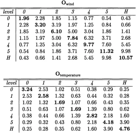
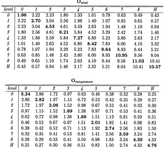
3.1 Observation error covariance matrices for simulated rawinsondes in the 3DVAR data assimilation at the standard resolution. . . . . 42 3.2 Observation error covariance matrices for simulated rawinsondes in the

3DVAR at double resolution . . . . 43 3.3 Vertical background error correlations in the standard resolution 3DVAR. 48 3.4 Vertical background error correlations in the double resolution 3DVAR. 50 4.1 Matrices used to generate simulated rawinsonde observation errors at the

standard resolution. . . . . 71 4.2 Matrices used to generate simulated rawinsonde observation errors at

dou-ble resolution. . . . . 72 8.1 Means and standard deviations of domain-averaged analysis and 3 day

forecast errors for different fixed observation networks during a 360 day tim e series. _{. . . 156} 8.2 As in Table 8.1, for 1 or 2 single observations added to 16 fixed observations. 158 8.3 As in Table 8.2, for 1 cluster 3 observations added to 16 fixed observations. 164 8.4 As in Table 8.2, for 2 single observations added to 64 fixed observations. 166 9.1 Maximum improvements and degradations in analyses and forecasts

pro-duced by adding a cluster 13 of observations to 16 fixed observations at day 2.5. . . . 188 9.2 Maximum improvements and degradations in analyses and forecasts

pro-duced by adding single or clustered observations to fixed observation dis-tribution 1 at day 2.5. . . . 201

(14)

(15)

Chapter 1 Introduction

1.1 Motivation and background

For several decades, it has been known that numerical weather forecasts are sen-sitive to small changes in initial conditions. This means that even if we could model the atmosphere perfectly, errors in the initial conditions would amplify rapidly, leading to forecast errors and forecast failures. The initial conditions for operational numeri-cal weather prediction (NWP) models, numeri-called analyses, are based on a combination of short range numerical forecasts with observations. The observations, where available, constrain the atmospheric state in the forecast model to be as close as possible to the true atmospheric state. The current observation network is made up of three types of observation platforms. Fixed platforms, such as rawinsonde stations, take observations at pre-selected times and locations, generally near population centers and thus over land. In the data gaps left by the fixed network, there are observations taken from platforms of opportunity, such as planes and ships, and from remote sensing platforms. At any given time, however, these latter two types of platforms are usually at locations which were selected for reasons other than weather prediction. In many cases, they also have limited vertical coverage or resolution.

Because the observation network is inhomogeneous, in any forecast situation there will be regions where information about the initial conditions is important but where there are insufficient observations. If we could use our knowledge about a specific atmo-spheric situation to identify these regions, it might be possible to deploy programmable observation platforms to take data in them and improve the initial conditions. These adaptive (also called targeted) observations could both reduce global analysis errors and

(16)

help predict important weather phenomena on various temporal and spatial scales. Forecasts will probably benefit little from observations in regions where the initial conditions are already quite accurate or where errors will have only a small effect on forecasts which interest us. Thus, effective adaptive observation strategies are likely to incorporate information both about probable analysis errors and about rapidly amplify-ing forecast errors. Various strategies have been proposed to include these criteria, each assuming that somewhat different analysis and forecast errors are the most important to identify and correct first. Subjective methods, such as identifying tropopause or other features which may be pre-cursors of rapidly developing atmospheric systems in data sparse areas, have been suggested (e.g. Snyder 1996). However, because it is not always possible to subjectively identify important features for a certain forecast (for example, when there is downstream energy propagation), several objective techniques have been proposed for adapting observations.

Each individual implementation of each adaptive observing strategy is different, and so we do not discuss the specific proposed strategies in detail. As an overview, however, the objective strategies which are currently being developed and tested include three ba-sic types. First, there are techniques based primarily on estimates of errors in the initial conditions, such as the methods using ensemble spread tested in Lorenz and Emanuel (1998). Second, strategies have been developed directly from adjoint techniques, cal-culating optimal perturbations (singular vectors) or sensitivities of forecasts to small changes in the initial conditions (e.g. Bergot et al. 1999, Gelaro et al. 1999, Palmer et al. 1998). Adjoint-based targeting strategies emphasize the errors which, if they exist in the initial conditions, will grow most rapidly. Although error statistics can be incorporated, the current implementations of adjoint-based strategies include little or no information about the probability of analysis and forecast errors. Finally, there are strategies which explicitly combine the error probability and error growth criteria. The ensemble trans-form technique, for example, uses an ensemble of perturbed forecasts to estimate both uncertainty in analyses and forecasts and the time evolution of the uncertainty (e.g. Bishop and Toth 1996, Bishop and Toth 1999).

Intuitively we believe that the best strategies will combine the two criteria in some manner. Unfortunately, adapting observations successfully has turned out to be a much more complex exercise than simply evaluating one or both of the criteria in the the-oretically optimal way. How much the different strategies improve forecasts in any atmospheric situation depends on many factors, including the selected "forecast of in-terest," the limitations of the observing platforms, and the data assimilation procedure

(17)

which incorporates the observations into the model state to create the initial conditions for forecasting. This means that the best strategies are likely to vary from situation to situation, and that they are likely to change as forecast models, available observing platforms, and data assimilation schemes evolve. At this time, it is not clear which (if any) of the currently proposed adaptive strategies will be most beneficial in any situation and implementation.

Current work on adaptive observations includes several different approaches, ranging from field experiments in which observations are taken to improve weather forecasts in real time, to idealized studies with simple models. In the real atmosphere, targeted observations are being implemented for tropical cyclone forecasts (Burpee et al. 1996, Aberson 1997; S. Aberson, personal communication), as well as being tested for mid-latitude weather forecasts during the Fronts and Atlantic Storm Track Experiment (FAS-TEX, in Jan.-Feb. 1997) and the North Pacific Experiment (NORPEX-98, in Jan.-Feb. 1998; NORPEX-99, to occur in Jan.-Feb. 1999). Several types of additional observing platforms have been tested, including dropwindsondes released from aircraft and high-resolution winds derived from satellite water vapor data (Velden et al. 1997), with data potentially gathered from unmanned aircraft in the future (Langford and Emanuel 1993). Unfortunately, because observing platforms and forecast verifications are often highly constrained in the real world, it is difficult to obtain enough good cases to allow one to draw firm conclusions. In addition, operational forecasting systems are complex, data assimilation systems and forecast models vary between numerical weather prediction centers, and the range of possible forecasting goals is large. This combination of factors make the results from real world adaptive observations difficult to interpret. The results are preliminary, and we do not discuss them in detail. In general, however, it is clear that so far the real adaptive observations have had a mixed influence. The assimilated extra observations have improved some forecasts, but in other cases they have had little impact or have even degraded forecasts (see Emanuel and Langland 1998, Gelaro et al. 1999, Langland et al. 1999a, and Szunyogh et al. 1999 for sample FASTEX results; see Langland et al. 1998b and Toth et al. 1999 for initial NORPEX results).

To eliminate many of the practical constraints, observing system simulation experi-ments (OSSE's) use a forecast model and a data assimilation system to simulate obser-vations and an analysis and forecast cycle. Because simplifying the forecast model both reduces the computational cost dramatically and makes the understanding the results easier, several of these idealized studies have been performed with low-order models. Lorenz and Emanuel (1998), for example, used a one-dimensional model, which predicts

(18)

one quantity at 40 locations on a latitude circle, to investigate several adaptive obser-vation strategies. Berliner et al. (1999) proposed a statistical framework and used it with the same one-dimensional model to explore several aspects of observing networks. These and similar experiments have suggested that adapting observations may be ben-eficial and have raised some important issues to consider when adapting observations. However, because of the one-dimensional dynamics of the model and the associated lack of requirement for a complex data assimilation system, these results may only apply to real atmospheric forecasts in a limited sense.

Both the idealized simple model and the real world approaches have left unanswered several important questions about adaptive observations. Although these questions are much too broad and complex to answer completely within the scope of this study, we begin to address them with the hope that our results will further our theoretical and practical understanding of how we can use observations to improve weather forecasts. This both can help us interpret results from other adaptive observations studies and can suggest which issues are the most important to explore first in future studies. The questions we address are:

" Can adaptive observations improve analyses and forecasts on a statistically sig-nificant basis, in a fully three-dimensional dynamical system with a realistic data assimilation system? If adapting observations can improve analyses and forecasts, what kinds of improvements can we expect under different circumstances?

* Which types of strategies are likely to be the most effective in different circum-stances? How can the strategies best be implemented, in terms of allocation of observational resources in space and time? How effectively can we estimate errors in initial conditions for use in adaptive observation strategies?

" How important are the limitations of the data assimilation system for adapting observations? How would we like to change the data assimilation procedure to improve the influence of observations on forecasts?

" How important is the risk of degradations when taking extra observations? How can we minimize the risk? With this risk in mind, what is the best way to define our goals when trying to optimally allocate observations?

* Given that we have limited observational resources, as discussed in Emanuel et al. (1997), what is the "optimal" mix of observing systems? In other words, what

(19)

role would we like all different types of observations, adaptive and non-adaptive, to play in the future?

The adaptive observing framework for addressing these issues is fairly new. Some of the more basic underlying questions, however, have been addressed previously from somewhat different perspectives. For example, it has recently come to our attention that during the late 1960's and early 1970's, several studies were performed with OSSE's to investigate which types of observations are the most useful for NWP and how these observations can best be assimilated, questions reminiscent of several of those above. More precisely, as satellite data first became available and as optimal interpolation data assimilation schemes became more accepted, several researchers began to explore how asynoptic data (primarily satellite but also including aircraft and other in situ data) might compare to and fill in gaps left by more traditional land-based radiosonde observations. Some of the studies focussed on comparing forecasts from initial conditions generated with observations distributed differently in space and time (Bengtsson and Gustavsson 1971, Bengtsson and Gustavsson 1972, Charney et al. 1969, and Morel et al. 1970). Other studies focussed on prioritizing data types, considering different observing platforms which could observe different meteorological variables with different accuracies (Charney et al. 1969, Jastrow and Halem 1970, Smagorinsky et al. 1970). These early studies were limited by the lack of computational resources; the forecast models are simple and their resolutions coarse by current standards, and only a few experiments could be run. Although the specific issues addressed in these studies are different, some of the general goals and methods are similar to those we use.

1.2 Approach

We use an approach which bridges the gap between the full numerical weather predic-tion system and the idealized simple model experiments described above: an idealized OSSE setup with a fully three-dimensional, yet simplified, quasi-geostrophic forecast model and a realistic data assimilation system. The basic framework for the experi-ments follows that used by Lorenz and Emanuel (1998) and previous observing system simulation studies (e.g. Jastrow and Halem 1970). We have selected an OSSE setup to avoid many of the logistics which make improving real-time forecasts difficult. With repeatable experiments, simulated observations, and perfect knowledge, we are limited neither by the number of possible cases nor by our ability to sample those cases well.

(20)

Later, if we wish, some of the idealizations can be relaxed and the importance of the real-world constraints evaluated.

To address some of the issues raised by both the one-dimensional model and the real world studies, we decided to test different observing networks in a three-dimensional system, but one with as few competing processes as possible. For both our forecast model and for our "real" atmosphere, we chose an idealized multi-level quasi-geostrophic model. Because it has simplified forcing and geometry, the quasi-geostrophic model does not simulate some aspects of real mid-latitude synoptic behavior, such as storm tracks. In other respects, however, the model represents large-scale dynamics realistically, and its relative simplicity both makes a larger number of experiments computationally feasible and simplifies interpreting the results. Since the model dynamics have limited accuracy at synoptic scales, to the extent possible we do not interpret our results for sub-synoptic scale applications.

The forecast model cannot use the data without first incorporating it into a three-dimensional best estimate of the atmospheric state. Consequently, a data assimilation system is a necessary complicating factor. We developed a three-dimensional variational data assimilation system similar to those used in operational NWP so that we can begin to explore how any, necessarily imperfect, data assimilation system interacts with observations and with a forecast model. We describe the data assimilation system in detail, explicitly addressing the strengths and weaknesses of how it incorporates data. This helps us understand both how our choice of data assimilation systems might affect our results and how data assimilation techniques can be improved so that they use observations more effectively.

Originally we designed this study with the goal of determining the "optimal" adaptive strategy. As the study developed, however, it became apparent that this goal was not only impossible to achieve, but was also not the best goal to work towards, for several reasons. First, since the most effective strategy is likely to change from situation to situation and from forecasting system to forecasting system, it is not clear if there is such a thing as an optimal strategy. In addition, the proposed strategies are in early stages of development, both theoretically and practically, and thus did not seem ready for rigorous comparison. Finally, we realized that we understand very little about how any extra observations, adaptive or non-adaptive, interact with data assimilation systems, with forecast errors, and with forecast models. It therefore seemed unwise to compare strategies without understanding more fundamentally what happens to the observational data once they are taken.

(21)

As we moved towards understanding more fundamentally how observations are used by a forecast system, we also decided not to attempt explicitly to simulate real observing networks and real observing platforms. Thus, we did not implement a complex "stan-dard" background observation network, varying in time and with different observation densities in different pre-specified regions. Instead, we chose to test only idealized non-adaptive observation strategies. Rather than implementing one or more of the specific proposed adaptive observation strategies described above, we also decided to test only very simple adaptive strategies. The idealized observation strategies allow us to pro-duce results more general than a comparison of how specific strategies added to a given background network of observations can improve specific forecasts in specific forecasting systems.

The primary stated goal of adaptive observations is to improve important forecasts. However, to help us identify the key considerations for adapting observations in general, in this study we also test only idealized error norms. Most of the results presented are aggregated over a large number of cases, in terms of domain- and time-averaged analysis error. These results are still relevant for reducing forecast errors on average because, as we discuss in Section 5.2, in this simulated system average analysis improvement and average forecast improvement are linked. Improving forecasts in individual cases is a more complex issue, one which we only begin to address specifically towards the end of the study.

Adapting observations combines several different areas of numerical weather pre-diction, including data assimilation techniques, forecast error evolution, ensemble fore-casting, and adjoint techniques (including singular vectors). Although these topics are important background material for understanding adaptive observations, each is a broad and complex field on its own. Therefore, in the interest of space, we only discuss them briefly where relevant, directing the reader to some sample appropriate references for further information. To tie our results to real world forecasting, it is also important to have a basic understanding of several other issues, such as the currently proposed adaptive observation techniques and the influence of the adaptive observations tested in field experiments. Because these fields are new and evolving rapidly, and because many of the results are preliminary, again we do not discuss them in detail. When possible, we provide references for the adaptive observations results, although many of them are not yet published (as of late 1998). Often, however, our understanding of the important issues for adapting observations is not based on a single identifiable research study or researcher. Much of our interpretations of how our results might be applied to

(22)

real forecasting have developed from our experiences taking data and verifying forecasts during FASTEX (Joly et al. 1997, special issue of Quart. J. Roy. Meteor. Soc. to ap-pear) and NORPEX-98 (Langland et al. 1999b) and from presentations and discussions from several workshops on targeted observations. These workshops include those which took place: in Camp Springs, MD on 10-11 Apr. 1997; in Monterey, CA on 8 Dec. 1997 (summarized in Emanuel and Langland 1998); in Toulouse, France on 27-30 Apr. 1998; and in Monterey, CA on 4-5 Nov. 1998 (summary in preparation by R. Langland).

The results from the quasi-geostrophic model, the idealized experimental setup, and the simplified strategies cannot be applied directly to real forecasting. They are im-portant, however, because they can help us understand fundamental aspects of how any atmospheric or related forecasting system might respond to different types of ob-servational information. The basic principles learned from the experiments with the simplified model can then be tested with a more complex, more realistic model and eventually explored with real atmospheric data.

1.3 Outline

In Chapters 2 and 3, the quasi-geostrophic model and three-dimensional variational data assimilation system are described. Chapter 4 explains the OSSE setup and how the observation strategies were chosen and implemented. Chapter 5 presents results from networks with different densities of fixed observations, including a summary of the sensitivity of the results to the error norm and to the data assimilation procedure. From these results, we develop a framework for studying further changes in observation networks. We then begin to address the issues discussed above, building on the low-order model results and investigating some unresolved difficulties with adapting observations from the field experiments.

In Chapter 6, we compare global idealized adaptive observations to non-adaptive global observation strategies at different observation densities. We then explore how a limited amount of observational resources might be optimally allocated in space and time. Chapter 7 tests using different-sized ensembles to estimate background error for adaptive observations. We also briefly discuss how the results may be affected if obser-vation locations must be selected well in advance of the obserobser-vation time. In Chapter 8, observation strategies are tested when the observations are added to a pre-existing net-work of fixed observations. The influence of the extra observations is illustrated both

(23)

with time-averaged results and with results from a time series of individual situations. Finally, in Chapter 9, we present examples and statistics of how individual extra obser-vations affect analyses and forecasts in specific cases. These results demonstrate some of the specific ways in which observations can interact with errors in the initial conditions, with the data assimilation system, and with the forecast model.

Throughout the study, we discuss the extent to which we believe the results from the simplified model and the simplified experimental setup may or may not apply to more complex systems and to more general situations. We also explore the importance of the data assimilation system for the results, and we address what next steps are required before our results can be applied to real world observing networks.

(24)

(25)

Chapter 2 Quasi-geostrophic

model

The quasi-geostrophic (QG) model used is a gridpoint channel model on a beta plane, periodic in longitude, developed at the National Center for Atmospheric Research (NCAR) and described in Rotunno and Bao (1996, hereafter referred to as RB96). We have selected this multi-level QG model because it exhibits three-dimensional dynamical behavior that is, to first order, similar to that of the real atmosphere, while it remains simple enough to make a large number of runs computationally feasible. The QG model is forced by relaxation to a specified zonal mean state (described below); it has no orogra-phy or seasonal cycle. Dissipation includes fourth-order horizontal diffusion and, at the lower boundary, Ekman pumping. The version for this study has constant stratification and a tropopause with fixed height (but varying temperature) at the upper boundary

z = H. With the simplified geometry and forcing, this QG model does not simulate

some features of real mid-latitude synoptic behavior, such as storm tracks and other stationary wave patterns. Even so, the model exhibits a wide range of chaotic behavior. We have chosen an idealized QG model to help us to gain a basic understanding of how observation networks behave, an understanding which we can later apply to adapting observations in a more complex, more realistic atmosphere.

The QG model variables are potential vorticity (q) in the interior and potential temperature (0) at the upper and lower boundaries. With the geopotential V) (referred to as streamfunction once non-dimensionalized) and the geostrophic wind vg given by

0 = , (2.1)

g az'

and

(26)

we define the pseudo-potential vorticity as

1

f

a20

q + #y. (2.3)

f N2 oz2

The equation governing the interior potential vorticity, including the diffusion and re-laxation, is then

a

1 (-

+ Vg - V) q = -vV 4q - (q - gre). (2.4)

at Trelax

With Ekman pumping at the lower surface, the equation for the potential temperature at the upper and lower boundaries is

SvNV)O=

v 4o2 ( at z = 0

(-+vg-V6=- V0- (O -GrefV{ - 9 (2.5)

jt _Trelax ₀

at z = H, where the vertical component of the geostrophic vorticity is defined as

av

_ u_

C= g_

aUg

(2.6)

and Av is the vertical eddy diffusion.

The zonal mean reference state (qref, Oref) is a Hoskins-West jet (Hoskins and West

1979), with a zonal wind (u) maximum at the tropopause, u = 0 at the channel walls, and a corresponding sinusoidally varying meridional temperature gradient. The jet is specified according to Equation (17) in Hoskins and West (1979); for further details on the mathematical formulation, see Hoskins and West (1979) and RB96. In the results below, the maximum zonal wind speed U of the reference state jet is scaled to 60 ms- 1_,

and the model state is relaxed to the reference state over a time scale Trelax = 20 days.

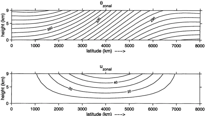
Figure 2.1 depicts meridional cross-sections through the reference state for the potential temperature and zonal wind profiles.

The diffusion coefficient v is set to 9.84 x 1015 m4s-1 for the standard resolution runs. Defining the damping time scale for a wavenumber k as

1 Tdiff = 0V

the damping time scale for the shortest wave at the standard resolution (wavelength

= 2Ax = 500 km) is approximately 1 hour.

(27)

0zonal --C --- ---0 0 1000 2000 3000 4000 5000 6000 7000 8000 latitude (km) ---- > t zonal -I I I _ 40 -C 0 1000 2000 3000 4000 5000 6000 7000 8000 latitude (kin) --- >

Figure 2.1: Meridional cross-section through the zonal mean reference state for (a) potential temperature (K) and (b) zonal wind (ms-1_{) in the QG model.}

formula for the surface stress, as in RB96. Following Valdes and Hoskins (1988), the viscous boundary layer can be made equivalent to an explicit Ekman layer with a no-slip lower boundary condition. The vertical eddy diffusion coefficient Av is related to the surface drag coefficient cD by

cD IUsurf = 2

where Iusa I is the average total horizontal surface velocity. We set Av = 5 m2s-1, which is equivalent to cD P 1.5 x 10-3 and IUsurf

I

10ms- 1. Av is also related to the traditional Ekman number Ev according to

E, = 2 Av

f H2

The equations are non-dimensionalized as in RB96, and at each time step, the bound-ary potential temperature is incorporated into the interior potential vorticity and Equa-tion (2.3) is inverted to solve for

4.

Through Equation (2.1), the boundary potential temperature determines the upper and lower boundary conditions for the inversion. Par-titioning the streamfunction into

4

(the time-varying zonal mean component) and 0'

(28)

(the deviation from

4),

the boundary conditions at the channel walls are

0 (2.7)

at ay'

0, (2.8)

and no diffusion, i.e.

v =0. (2.9)

After the streamfunction is diagnosed, Equations (2.4) and (2.5) are integrated forward in time using leapfrog time differencing, except just after a new analysis is created, when a forward Euler scheme is used. The time step is approximately 30 minutes for the standard resolution runs, and the integration is time filtered to remove the computational mode (Robert 1966).

The dimensional domain for all results shown has a circumference of 16000 km and a channel width of 8000 km (approximately 700 latitude, large enough so that there is less interaction between the synoptic systems and the channel walls). The depth H is 9 km. The Rossby radius of deformation is defined as

Rd NH (2.10)

f

With the Brunt-ViiissIl frequency N = .011293 and

f

= 1 x 10-4, Rd r 1000 km. The Rossby number is defined as

Ro U U (2.11)

fL NH'

and since U = 60 ms-1, R. ~ .59. The advection time scale

L 1

tadv = - =f~ (2.12)

U

f

Ro is then approximately 5 hours.

The standard resolution runs have 250 km horizontal resolution and 5 vertical levels. At this resolution, we have estimated from the growth rate of small differences in the QG model state that the error doubling time is approximately 2.5-4 days (for example, compare for dense observations the average magnitude of the initial condition errors in Figure 5.1 with that of the 5 day forecast errors in Figure 5.3). The specific error growth rate depends on the situation, but this value may be on average slow compared to the

(29)

real atmosphere. If the resolution is roughly doubled to 125km horizontal resolution and 8 vertical levels, changing to a 7.5 minute time step and a diffusion coefficient v = 2.46 x 1015 m4s-1, the corresponding error doubling time is 1-2 days. To evaluate how sensitive the results are to the model resolution and to the error growth time scale, Section 6.4 presents a few of the results at double resolution. Since it was not computationally feasible to run all of the experiments at higher than the standard resolution, however, we have also compensated for the somewhat slow error growth rate by changing the rate at which observational data are input into the model in Sections 5.4 and 6.3

Figure 2.2 shows the streamfunction and the potential temperature at the upper and lower boundaries for an arbitrarily selected sample QG model state at the standard resolution. Figure 2.3 shows the same fields for an arbitrarily selected state at double resolution. The QG model at higher resolution not only has faster error growth, but comparing Figures 2.2 and 2.3, we see that it also better resolves strong temperature gradients and thus has a more focused jet stream.

(30)

sb: tr DAY

CONTOUR FROM -0.60000 TO 0.50000 CONTOUR INTERVAL OF 0.500OOE-01 PT(3.3)= 0.15151

st: tr DAY 0.00

CONTOUR FROM -1.6000 TO 1.8000 CONTOUR INTERVAL OF 0.20000 PT(3.3)= 1.8049

Figure 2.2: Sample vertical cross-sections through the standard resolution QG model state at an arbitrary time, for non-dimensionalized: (a) lower boundary streamfunction, (b) upper boundary streamfunction, (c) lower boundary potential temperature, and (d) upper boundary potential temperature. Longitude (periodic) is plotted on the x-axis and latitude is plotted on the y-axis, each with resolution 250 km.

(31)

tb2:

tr

DAY

0.00

CONTOUR FROM -1.2000 TO 1.4000 CONTOUR INTERVAL OF 0.20000 PT(3.31= 1.4193

tt2: tr DAY

0.00

CONTOUR FROM -1.B000 TO 1.8000 CONTOUR INTERVAL OF 0.20000 PT(3,3)= 1.9827

(32)

sb:

tr

DAY

0.00

CONTOUR FROM -0.80000 TO 0.55000 CONTOUR INTERVAL OF 0.50000E-01 PT(3.3)= 0.14986

st: tr DAY

0.00

CONTOUR FROM -1.8000 TO 1.4000 CONTOUR INTERVAL OF 0.20000 PT(3,3)= 1.3671

Figure 2.3: Sample vertical cross-sections through the double resolution QG model state at an arbitrary time, for non-dimensionalized: (a) lower boundary streamfunction, (b) upper boundary streamfunction, (c) lower boundary potential temperature, and (d) upper boundary potential temperature. Longitude (periodic) is plotted on the x-axis and latitude is plotted on the y-axis, each with resolution 125 km.

(33)

tb2:

tr

DAY

0.00

CONTOUR FROM -1.2000 TO 1.0000 CONTOUR INTERVAL OF 0.20000 PT(3.3)= 1.0625

tt2: tr DAY

0.00

CONTOUR FROM -1.8000 TO 1.8000 CONTOUR INTERVAL OF 0.20000 PT(3.3)= 1.7402

(34)

(35)

Chapter 3 Data assimilation

The data assimilation system controls how observations are incorporated into the forecast model, and therefore it is a key aspect of any data impact study using a rela-tively complex model. For the initial evaluation of observation strategies, we have im-plemented a three-dimensional variational (3DVAR) data assimilation scheme, based on the Spectral Statistical-Interpolation (SSI) analysis system currently operational at the National Centers for Environmental Prediction in the U.S. (Parrish and Derber 1992), and similar to those operational at many other weather prediction centers. Although more sophisticated data assimilation systems are currently being developed and imple-mented, we have selected 3DVAR as the baseline data assimilation system because it has been well-tested, it is similar to operational schemes, it is computationally less intensive than more complex schemes, and it simplifies understanding how the data assimilation affects the observations. Further details on other possible data assimilation schemes and our choice of 3DVAR are discussed in Section 3.1. Sections 3.2, 3.3, and 3.4 present the 3DVAR algorithm and describe its implementation in this study. In Section 3.5, we show several examples of how the 3DVAR assimilates the observations.

3.1 Choice of data assimilation

In this section, we briefly outline several different atmospheric data assimilation techniques and explain why we chose to implement 3DVAR. Because data assimilation is a large and rapidly developing field, with each data assimilation implementation slightly different, we have discussed only a few basic atmospheric data assimilation formulations and have avoided going into much detail. For further information on the theory used

(36)

to develop variational data assimilation (e.g. Bayesian estimation) and statistical data assimilation in general, the reader is referred to Bengtsson et al. (1981), Daley (1991), and Lorenc (1986), and references therein. For more information on advanced data assimilation topics, the reader is referred to the references listed in Courtier et al. (1993). 3DVAR is described in greater detail in the remaining sections of this chapter, and for details on the other specific data assimilation algorithms discussed, a few sample references are given in the text.

Until several years ago, optimal interpolation (01) schemes were used to assimi-late data at most operational weather prediction centers (e.g. Lorenc 1981). In theory 3DVAR and 01 are quite similar. In practice, however, most 01 implementations solve several local assimilations, selecting a relevant subset of the observations for each region, while 3DVAR and related variational data assimilation schemes solve for the analysis globally, incorporating all available data at once. The different formulation of 01 creates analyses which can be easier to attribute to features in the background field and in the observations. Recently, however, operational centers have been moving away from 01 toward variational data assimilation (e.g. Parrish and Derber 1992), and we have chosen 3DVAR for similar reasons. First, 01 requires a data selection algorithm, which can be complex and difficult to implement, and which can produce analyses that are inconsis-tent between regions. In addition, since the 3DVAR analysis is global and is formulated in terms of the analysis variables instead of in terms of pre-defined observation variables, 3DVAR can more easily be adapted to incorporate a variety of data sources (Parrish and Derber 1992). The basic 3DVAR algorithm can also easily be modified to include additional constraints on the analysis, such as a balance condition or other dynamical constraint. Because of this flexibility, we can later adapt the 3DVAR framework to any data assimilation algorithm that can be posed variationally.

Atmospheric variational data assimilation uses predicted error statistics to weight a forecast model state or model trajectory (called the background field) and observa-tions. It then solves for the analysis which has the minimum difference from both the background field and the observations. Although the idealized formulation of variational data assimilation is theoretically appealing and is useful for small-order problems, it can-not currently be used to assimilate atmospheric data in realistic situations for two main reasons. First of all, in atmospheric 3DVAR the full algorithm contains O(N 2_{) error}

cor-relations, where N is equal to the number of analysis variables. In more sophisticated data assimilation formulations the algorithm can be even more complex, with operations on the O(N 2_{) values. Even in the simplified system studied here, N is O(104). Although}

(37)

we do not have to explicitly invert the equations, it is computationally very expensive to calculate or store all of the values, and it is at best infeasible to solve the full algorithm for a large number of experiments. In addition, because of the large number of error correlations and their detailed time-dependent structure, at each assimilation time very little is known about the error statistics which determine the weights for the inversion. Therefore, to implement a practical variational data assimilation for numerical weather prediction, we must generally simplify the basic algorithm.

Each type of data assimilation and each implementation makes different assumptions, and it is not yet clear which assumptions are the most valid or which work the best. For 3DVAR, we develop a feasible algorithm by simplifying the error statistics, particularly the structures of the background errors; the assumptions used in our version of 3DVAR are described in Section 3.4. Our 3DVAR behaves similarly to data assimilation systems at most operational weather centers. With only these simplified statistics, however, the 3DVAR has little knowledge of the atmospheric dynamics, and thus it is far from optimal. Several more complex data assimilation algorithms have been proposed to incorporate information about time- and space-dependent errors, and by doing so they can greatly improve how the data assimilation recreates the atmospheric state from the observations. To be feasible, these algorithms must be simplified even more than 3DVAR, but as computational resources increase, they will become possible for more implementations.

One possibility, the Kalman filter, has been applied in a variety of fields, and it may be useful for atmospheric data assimilation in a modified form (e.g. Ghil 1997 and refer-ences therein). The Kalman filter, instead of specifying the background error statistics externally (as in 3DVAR), uses the forecast model explicitly to update the statistics at each data assimilation time. A second example is four-dimensional variational data assimilation (4DVAR), which is similar to 3DVAR but minimizes in time as well as in space (e.g. Courtier and Talagrand 1987, Talagrand and Courtier 1987, and Thepaut et al. 1993). In 4DVAR the background field is a forecast model trajectory over a spec-ified time period instead of model state at a specific time. Both the Kalman filter and 4DVAR include adjoint models, and simplified forms of 4DVAR using an adjoint or a quasi-inverse model have also been proposed (e.g. Pu et al. 1997). Another possibility is the "ensemble Kalman filter," a 3DVAR-like algorithm which uses an ensemble of perturbed forecasts to estimate the correlations between errors in the background field in real time (Houtekamer and Mitchell 1998). Several other proposed data assimilation strategies, such as those which combine ensemble perturbations directly (K. Emanuel,

Adaptive observations : idealized sampling strategies for improving numerical weather prediction

Adaptive observations:

Idealized sampling strategies for improving numerical

weather prediction

Rebecca Elisabeth Morss

of

All

Adaptive observations:

Idealized sampling strategies for improving numerical weather

prediction

by

Rebecca Elisabeth Morss

Abstract

Acknowledgments

Contents

List of Figures

List of Tables

Chapter 1

Introduction

1.1

Motivation and background

1.2

Approach

1.3

Outline

Chapter 2

Quasi-geostrophic

model

g az'

f

a

1

(-

SvNV)O=

av

aUg

I

4.

4

4),

at ay'

f

f

tb2:

tr

DAY

0.00

0.00

sb:

DAY

0.00

0.00

tb2:

DAY

0.00

0.00

Chapter 3

Data assimilation

3.1

Choice of data assimilation