HAL Id: insu-01058954
https://hal-insu.archives-ouvertes.fr/insu-01058954
Submitted on 28 Aug 2014
HAL is a multi-disciplinary open access
archive for the deposit and dissemination of
sci-entific research documents, whether they are
pub-lished or not. The documents may come from
teaching and research institutions in France or
abroad, or from public or private research centers.
L’archive ouverte pluridisciplinaire HAL, est
destinée au dépôt et à la diffusion de documents
scientifiques de niveau recherche, publiés ou non,
émanant des établissements d’enseignement et de
recherche français ou étrangers, des laboratoires
publics ou privés.
Automatic recognition of T and teleseismic P waves by
statistical analysis of their spectra: An application to
continuous records of moored hydrophones
Alexey Sukhovich, Jean-Olivier Irisson, Julie Perrot, Guust Nolet
To cite this version:
Alexey Sukhovich, Jean-Olivier Irisson, Julie Perrot, Guust Nolet. Automatic recognition of T and
teleseismic P waves by statistical analysis of their spectra: An application to continuous records of
moored hydrophones. Journal of Geophysical Research, American Geophysical Union, 2014, 119 (8),
pp.6469-6485. �10.1002/2013JB010936�. �insu-01058954�
RESEARCH ARTICLE
10.1002/2013JB010936
Alexey Sukhovich and Jean-Olivier Irisson contributed equally.
Key Points:
• New automatic signal discrimination method is proposed
• The method uses Gradient Boosted Decision Trees
• Method can be useful in analysis of any large data sets
Correspondence to:
A. Sukhovich, sukhovich@univ-brest.fr
Citation:
Sukhovich, A., J.-O. Irisson, J. Perrot, and G. Nolet (2014), Automatic recognition ofTand teleseismicPwaves by statisti-cal analysis of their spectra: An applica-tion to continuous records of moored hydrophones, J. Geophys. Res. Solid
Earth, 119, doi:10.1002/2013JB010936.
Received 30 DEC 2013 Accepted 23 JUL 2014
Accepted article online 31 JUL 2014
Automatic recognition of T and teleseismic P waves
by statistical analysis of their spectra: An application
to continuous records of moored hydrophones
Alexey Sukhovich1, Jean-Olivier Irisson2,3, Julie Perrot1, and Guust Nolet4
1Domaines Océaniques, Université Européenne de Bretagne, Université de Bretagne Occidentale, CNRS, IUEM, Plouzané,
France,2Sorbonne Universités, UPMC, Université Paris 06, UMR 7093, LOV, Observatoire Océanologique,
Villefranche-sur-Mer, France,3CNRS, UMR 7093, LOV, Observatoire Océanologique, Villefranche-sur-Mer, France,4Géoazur,
Université de Nice, UMR 7329, Valbonne, France
Abstract
A network of moored hydrophones is an effective way of monitoring seismicity of oceanic ridges since it allows detection and localization of underwater events by recording generated T waves. The high cost of ship time necessitates long periods (normally a year) of autonomous functioning of the hydrophones, which results in very large data sets. The preliminary but indispensable part of the data analysis consists of identifying all T wave signals. This process is extremely time consuming if it is done by a human operator who visually examines the entire database. We propose a new method for automatic signal discrimination based on the Gradient Boosted Decision Trees technique that uses the distribution of signal spectral power among different frequency bands as the discriminating characteristic. We have applied this method to automatically identify the types of acoustic signals in data collected by two moored hydrophones in the North Atlantic. We show that the method is capable of efficiently resolving the signals of seismic origin with a small percentage of wrong identifications and missed events: 1.2% and 0.5% for T waves and 14.5% and 2.8% for teleseismic P waves, respectively. In addition, good identification rates for signals of other types (iceberg and ship generated) are obtained. Our results indicate that the method can be successfully applied to automate the analysis of other (not necessarily acoustic) databases provided that enough information is available to describe statistical properties of the signals to be identified.1. Introduction
The seismicity of the oceanic ridges and spreading centers is characterized by a large number of earth-quakes, most of which are not detected by land-based seismic stations due to their low magnitudes. To record these earthquakes, common approaches are the use of ocean bottom seismometers (OBSs) [Kong et
al., 1992; Wolfe et al., 1995; Bohnenstiehl et al., 2008]) or moored hydrophones [Dziak et al., 1995; Slack et al.,
1999; Fox et al., 2001; Smith et al., 2002; Simão et al., 2010]. In the second case, several (four and sometimes more) hydrophones form a network which surrounds the area of interest. Compared to the OBSs, which are deployed over areas of limited extent, a hydrophone network can allow the surveillance of sections of the mid-oceanic ridges several hundreds of kilometers long. The hydrophones are positioned near the axis of the SOund Ranging And Fixing (SOFAR) channel which acts as an acoustic waveguide [Munk et al., 1995]. Seismic events along the mid-oceanic ridges, while of low intensity, frequently produce acoustic waves of appreciable amplitude called T (short for tertiary) waves [Tolstoy and Ewing, 1950]. These waves enter the SOFAR channel and, thanks to its waveguiding properties, can propagate long distances with almost no attenuation [Okal, 2008] and be recorded by the hydrophones. When a T wave is detected by a network of hydrophones, the coordinates of the spot where conversion of seismic to acoustic waves has taken place can be found [Fox et al., 2001]. During the last decade, hydrophone networks have detected many more events produced along the mid-oceanic ridges as compared to the land-based stations [Bohnenstiehl et al., 2003; Goslin et al., 2012]. The usefulness of hydrophone data is not limited to studies of the oceanic seis-micity. For example, acoustic signals generated by teleseismic P waves were also observed in hydrophone records [Dziak et al., 2004]. The arrival times of these signals can be used in global seismic tomography whose progress is currently impeded by a lack of seismic data collected at sea [Montelli et al., 2004]. In all observational experiments with moored hydrophones, the monitoring of the acoustic pressure vari-ation is done continuously. Because of the high cost of ship time instrument deployment and recovery are
Journal of Geophysical Research: Solid Earth
10.1002/2013JB010936
separated by long time periods, normally a year or even longer in some cases, which results in very large data sets. The very first step in the analysis of the recovered data sets consists of finding all recorded T waves (or other signals of interest) which has to be done manually by a human observer. This preliminary part is extremely time consuming due to the large amount of the data. Automatic signal identification is there-fore highly desirable. Matsumoto et al. [2006] have proposed a simple algorithm to perform an automatic detection of T waves by autonomous underwater robots. Recently, Sukhovich et al. [2011] have developed a probabilistic method for use on similar floats dedicated to record acoustic signals generated by teleseis-mic P waves [Simons et al., 2009; Hello et al., 2011]. While showing promising results, these methods are not quite universal as they require separate tailoring of their parameters for the detection of signals of a given type. Once adjusted, these methods discriminate one signal type from the rest. In another approach, sev-eral authors used neural networks, which is a machine learning technique, for automatic picking of onset times of P and S waves [Dai and MacBeth, 1997; Zhao and Takano, 1999; Gentili and Michelini, 2006]. In this paper, we report on a new automatic method based on a different machine learning technique, Gradient Boosted Decision Trees [Breiman et al., 1984; Friedman, 2002], that is also adept at classifying multidimen-sional data. Compared to the neural networks, this technique is less opaque in the sense that one always has complete information on each decision tree. Combined for all trees, this information allows one to calculate, for example, the effect of a single discriminating variable or the joint effect of several variables. Similar to the method of Sukhovich et al. [2011], our method uses the information on the distribution of the signal spectral power among different frequency bands; in contrast to Sukhovich et al. [2011], the use of Gradient Boosted Decision Trees (GBDT) allows classification of several signal types simultaneously. We have applied the new method to the data recorded by two moored hydrophones of the Seismic Investigation by REcording of Acoustic Waves in the North Atlantic (SIRENA) network which operated during the years 2002 and 2003 [Goslin et al., 2012].
The paper is structured as follows. First, a brief description of the method is provided. Afterward, a presen-tation of the hydroacoustic experiment SIRENA and details on the data processing are given. The results are presented in the next section, followed by the conclusions.
2. Method Description
We discriminate between various signal types by exploiting differences in signal spectra. More specifi-cally, the spectrum of each signal is characterized by the distribution of the spectral power among a set of frequency bands. These power distributions are used as discriminatory variables in a supervised classifica-tion procedure. In supervised classificaclassifica-tions, one first uses signals of known types to construct a statistical model which describes the differences between the types. This statistical model is then used to predict the most likely types of new, unknown signals. The techniques used to extract the spectral power distribu-tions (wavelet analysis) and to perform the supervised classification (GBDT) are presented in secdistribu-tions 2.1 and 2.2, respectively. Only a general description of GBDT is provided since its complete treatment goes far beyond the scope of this paper. For more details, we refer the reader to Natekin and Knoll [2013], which is an excellent tutorial with several illustrative examples.
2.1. Signal Processing
The spectral power distribution as a function of a frequency band is estimated with the help of the dis-crete wavelet transform (DWT), similar to the procedure described by Sukhovich et al. [2011]. For the sake of completeness, we provide here a brief description. The wavelet transform is analogous to the Fourier Transform (FT) in the sense that a given signal is projected onto a space defined by a set of elementary functions called wavelets [Jensen and la Cour-Harbo, 2001]. As a result, a set of wavelet coefficients is pro-duced. It is important to note that contrary to sines and cosines which are elementary functions of the FT, wavelets are functions of two variables, frequency and time. Thanks to this fact, the DWT allows the obtain-ing of the information on the spectral content of the signal both in the time and frequency domain, similar to the Short-Time Fourier Transform (STFT, also known as spectrogram). The difference between the two is that the DWT is nonredundant: it produces exactly the same number of wavelet coefficients as the length of the signal to transform, while the STFT calculates FTs of overlapping (usually by 50%) time windows. The DWT thus requires significantly fewer calculations. Besides helping to speed up the analysis, this reduction in calculation time is of great importance when the analysis is done in situ on the platforms with limited amount of power available [Simons et al., 2009]. Another attractive feature of the DWT is the existence of
Figure 1. Representative acoustic signals of (left, top) teleseismic P wave and (right, top) T wave recorded by
hydrophone S5 of the SIRENA network. The signals are downsampled to 80 Hz. (middle and bottom) Signals’ scalogram and spectrogram. Scalogram pixels give positions of wavelet coefficients in a scale-time plane. Scale 1 corresponds to frequency range approximately between 20 and 40 Hz, scale 2 to frequencies between 10 and 20 Hz, and so on. Both absolute values of the wavelet coefficients and the spectral density are measured in the units of the standard deviation (from the mean).
simple and easy-to-program algorithms for its calculation. In particular, we are using the “lifting” algorithm [Sweldens, 1996].
Wavelet transforms use the notion of a“scale” rather than frequency. In some sense, the wavelet transforma-tion is also analogous to a filter bank analysis, with overlapping filters covering different frequency bands [Jensen and la Cour-Harbo, 2001]. During wavelet transformation, every iteration produces a set of wavelet coefficients for one scale, with each scale corresponding to a particular frequency band. As a rule of thumb, each subsequent scale has a passband centered around a frequency that is half of the center frequency of the previous scale. The first scale corresponds to the upper half of the total frequency band allowed by the sampling frequency Fs, approximately between frequencies Fs∕4 and Fs∕2. The second scale corresponds
to the lower frequency band lying approximately between frequencies Fs∕8 and Fs∕4 and so on for
subse-quent scales. Numerous wavelet bases exist, and the most suitable one is chosen for a particular problem at hand. We use a biorthogonal wavelet basis with two and four vanishing moments for the primal and dual wavelets, respectively, which is commonly abbreviated as CDF(2,4) [Cohen et al., 1992]. As was shown pre-viously [McGuire et al., 2008; Sukhovich et al., 2011], this wavelet construction provides a good compromise between computational effort and the filtering performance of the wavelets.
A convenient way to visualize the result of the wavelet transformation is a scalogram, which presents the absolute values of the wavelet coefficients in a time-scale plane. Figure 1 shows representative signals of teleseismic P and T waves along with their scalograms. The absolute value of a wavelet coefficient is propor-tional to the spectral power of the signal at the corresponding moment of time and scale. We use this fact to define an estimate skof the spectral power at the scale k as the average of absolute values of the wavelet coefficients at this scale:
sk= 1 Nk Nk ∑ i=1 |wk i| , (1) where wk
i is a wavelet coefficient, Nkis the number of the wavelet coefficients, and indices i and k number
Journal of Geophysical Research: Solid Earth
10.1002/2013JB010936
Figure 2. Representative acoustic signals produced by (left, top) a passing ship and (right, top) an iceberg recorded
by hydrophone S5 of the SIRENA network. The signals are downsampled to 80 Hz. (middle and bottom) Signals’ scalo-gram and spectroscalo-gram. Both absolute values of the wavelet coefficients and the spectral density are measured in the units of the standard deviation (from the mean). The signals emitted by ships during the investigated period were quasi-monochromatic with a frequency of 8.5 Hz. As expected, the largest wavelet coefficients are located at the scale 3 (frequency range between 5 and 10 Hz approximately). On the contrary, iceberg-generated signals are extremely long and composed of several harmonics whose frequencies vary with time.
The detection of an arriving signal is ensured by monitoring the value of the ratio of short-term to long-term moving averages (STA/LTA algorithm) [Allen, 1978]. Equation (1) is evaluated for wavelet coefficients within a time window starting when the value of the STA/LTA ratio exceeds 2 (trigger threshold). After the trig-ger, both moving averages continue to be updated so that the STA/LTA ratio is affected by the triggering signal. The signal’s end is declared when the STA/LTA ratio drops below 1 (detrigger threshold). These two values were found to work quite well in most cases: a lower trigger threshold would significantly increase the number of triggers due to ambient noise fluctuations while a higher detrigger threshold would not allow us to capture the entire length of the signal. However, these values are not universal, and some adjust-ments might be required if noise properties vary significantly from one site to another. The duration of time windows used for calculation of the short- and long-term moving averages were 10 and 100 s, respectively. From equation (1), a set (or a vector) of scale averages skis obtained. This set of values characterizes
the absolute spectral power distribution among the scales and thus varies from one signal to another (of the same type) according to the signal-to-noise ratio. A more uniform characteristic is a relative power distribution Skfound by normalizing the vector skby its L1norm:
Sk= sk L1 , where L1= K ∑ k=1 sk . (2)
In other words, normalization by L1norm gives the percentage of the total spectral power contained in each
scale. The values of the Skvector are the characteristics of the signals needed for the GBDT procedure. Note
that in the original implementation, Sukhovich et al. [2011] perform another normalization: each element Sk
is divided by the corresponding element of the similar scale average vector calculated for the ambient noise record immediately preceding the STA/LTA trigger. This second normalization by ambient noise means that a pure noise record with no signal should give elements Skwhose values are close to 1 for all scales. We have
T waves P waves Ship−generated Iceberg−generated 0.0 0.2 0.4 0.6 0.0 0.2 0.4 S2 S5 1 2 3 4 5 6 7 1 2 3 4 5 6 7 1 2 3 4 5 6 7 1 2 3 4 5 6 7 SCALE NUMBER SCALE A VERA GE S k
Figure 3. Dependence of the scale averageSkon the scale number for the signals of different types (indicated on top of each panel) detected by hydrophones (top row) S2 and (bottom row ) S5. For a given signal type, a panel shows scale averages of all detected signals with scale averages of the same signal connected by lines. The distribution of the scale averages within the same scale is represented by a violin plot. The extent of the violin plot gives the range ofSkvalues while its width at a givenSkvalue is proportional to the number of signals having similar value. The thickest part of the violin plot thus gives the position of the peak of the distribution.
can be seen in Figure 2, these signals are very long and their amplitude fluctuates significantly with time. As a result, it was common for the trigger to occur in the middle of the signal so that, instead of the ambient noise, the record preceding the trigger contained the part of the same signal. The second normalization thus tended to “wash out” the distinctive features of iceberg-generated signals.
We illustrate the method using data from two hydrophones deployed as part of the SIRENA experiment (section 3). Figure 3 shows the distribution of the scale averages Skof four signal types observed in the
records of these hydrophones. It can be seen that statistical properties of T and teleseismic P waves are very different: while for T waves the spectral power is mostly concentrated at scales 3 and 4, for teleseismic
P waves most of the signal power is located at scales 5 and 6. For the remaining two types of signals, namely,
those generated by ships and icebergs, the most powerful scales are scales 3 and 4, respectively.
As explained in section 2.2, the GBDT technique performs discrimination by comparing scale averages for different signal types at each scale. In this sense, Figure 4 represents the same information as Figure 3 but in the way the technique “sees” it. In each panel, the distributions of Skare compared for the signals of different
types. The smaller the overlap between distributions, the more discriminative and useful for classification is the scale. As expected from Figure 3, distributions of scale averages of P waves are well separated from the rest of the signals at virtually all scales. The strong overlap of the distributions for T waves, ship-generated
Figure 4. Probability density functions estimated for allSkdistributions (represented by violin plots in Figure 3) of the signals detected by hydrophones (top row) S2 and (bottom row) S5. In contrast to Figure 3, which displays in each panel the distributions of scale averages of a single signal type for all scales, this figure compares the distributions of scale averages of all signal types at a single scale (indicated on top of each panel). To facilitate the visual comparison, the logarithm ofSkis plotted along the horizontal axis and each probability density function is scaled to a maximum value of 1. The smaller the overlap between the distributions at a given scale, the higher is the discrimination power of this scale.
Journal of Geophysical Research: Solid Earth
10.1002/2013JB010936
Figure 5. The classification procedure of an unknown signal illustrated on a simple decision tree. The tree was
con-structed on the training data set containingn = 10signals of four different known types. An unknown signal is classified by passing it through the tree and distributing it along the branches according to the values of its characteristics (indi-cated in the right upper corner). The composition of the group into which the signal is distributed defines the likelihood for this signal to be of each of the four types. These probabilities are indicated in the lower right corner.
signals, and iceberg-generated signals at certain scales signifies that the discrimination of these signals will be more difficult than that of P waves. It can also be seen that the scales 3 and 4 are likely to be the most discriminating ones, since all four distributions overlap least at these scales.
2.2. Signal Discrimination
To automatically identify the types of detected signals, we use Gradient Boosted Decision Trees. Before describing the GBDT technique, it is worth considering in some detail the basics of a classic decision (or clas-sification) tree [Breiman et al., 1984]. A single decision tree similar to those used in this paper is presented in Figure 5. A decision tree is essentially a set of rules according to which successive binary splits are performed with each binary split taking into account the value of one of the data characteristics. In our case, each sig-nal is described by seven characteristics which are seven values of scale averages Sk. The classification of
any data set member (a signal in our case) is performed by passing it through the tree and distributing it along the branches according to the values of its characteristics. The tree itself is defined during the “train-ing” phase, which is performed on a training data set (i.e., a data set whose elements are already classified; in our case it is a set of signals of known types). For each split, a dedicated algorithm tests the values of all characteristics and retains the one which results in the highest “purity” of the two new nodes (i.e., each node containing as many signals of the same type as possible). A tree can be grown until every signal is isolated in its own node, or, alternatively, the number of splits can be fixed a priori. Therefore, a decision tree is a
supervised learning technique: the procedure first “learns” on a training set how to discriminate the data
and then uses this statistical model (i.e., the tree) to classify new unknown data. In the example presented in Figure 5, the training set consists of 10 signals of known type (four T waves, three P waves, two ship-generated signals, and one iceberg-ship-generated signal). The constructed tree has two levels of binary splits, which separate the signals according to the values of scale averages at scales 6, 3, and 7. Note that the succession of splits enables us to take into account interactions between variables. In this particular exam-ple, the value of scale average at scale 3 is considered only when the value of scale average at scale 6 is ⩽ 0.15. The composition of any final group defines the likelihood for a classified signal to be of each type. In Figure 5, there are five signals in the second group: four T waves and one ship-generated signal with no
P waves or iceberg-generated signals. Therefore, an unknown signal which ends up in this group has a
prob-ability of 4∕5 = 0.8 and 1∕5 = 0.2 to be a T wave and a ship-generated signal, respectively, and zero probability to be either a P wave or an iceberg-generated signal. In consequence, it is classified as a T wave. Simple decision trees similar to that presented in Figure 5 are straightforward and easily readable, but they often have suboptimal predictive power. To improve the prediction, stochastic boosting procedures have proved successful [Friedman, 2001, 2002]. The general principle of boosting is to combine many successive
small trees instead of using one large tree. The first tree is fit on the training data, divides it into few groups, and provides a first broad level of information (probabilities for each type in this case). The next tree is fit to the residuals of this first model and so on. For each signal, the residual is a function of the differences between the truth (the actual category of the signal) and the prediction of the model (the probability of being in each category). The truth is also expressed in terms of probabilities. For a T wave, for example, it has the value of 1 to be a T wave and 0 to be anything else. If the predicted probabilities for this T wave are
pT = 0.8, pP = 0.05, pship = 0.08, and pice = 0.07, its residual after classification is a function of 1 − 0.8, 0.05 − 0, 0.08 − 0, and 0.07 − 0. Each successive tree is fit in such a way as to minimize the residuals of all the signals. During this minimization process, the amount of information contributed by each individual tree is controlled by a constant called “learning rate.” Using a small learning rate (usually much smaller than one) improves the generality and predictive power of the model, since only patterns occurring in many trees will emerge from the ensemble. Stochasticity is introduced by randomly selecting a part of the data (50% in our case) to build each successive tree. Therefore, here, each signal was classified on average 2000 times because we used about 4000 trees (see below). The probabilities resulting from each successive classifications are then combined to produce final probabilities to be in each category.
The absolute number of trees has no importance since the computing time is short, typically about a minute on a regular personal computer for the 4000 trees used in this study. However, if too many successive trees are combined, unimportant peculiarities of the training set will be included in the model, which will hinder its generality and predictive power. Therefore, in the GBDT procedure one needs to decide when to stop growing each individual tree, how many trees to combine, and how much the model should learn from each tree. Maximum predictive power is achieved with (i) individual trees large enough to account for interac-tions between characteristics but not too large to avoid extracting too much information in one tree, (ii) as many trees as possible, (iii) a very small learning rate for each tree. With seven variables, four levels of splits in each individual tree proved to be efficient. The learning rate was set to 0.001 which was small enough that a few thousand trees were needed to model the training data set correctly. With this choice of parameters, the optimal number of trees was determined by fivefold cross validation. More precisely, the training data were randomly split into five equal pieces, a model was fit on four of them, and several predictions were made on the fifth part, each prediction with an increasing number of trees. The discrepancy between the probabilities for each signal of being of each type predicted by the model and the actual type was quanti-fied as the residual deviance. Initially, the residual deviance decreases sharply as more trees are added to the model, because each new tree helps to better classify the data. But at some point, additional trees only very marginally decrease the residual deviance and just waste computational resources. In our case, this point was reached between 3500 and 4500 trees.
All computations were carried out in the open-source software R (version 3.0.1)[ R Core Team, 2013] with packages gbm (version 2.1) for GBDT [Ridgeway, 2013], reshape2 and plyr for data manipulation and automation [Wickham, 2007, 2011], and ggplot2 for graphics [Wickham, 2009].
3. Data
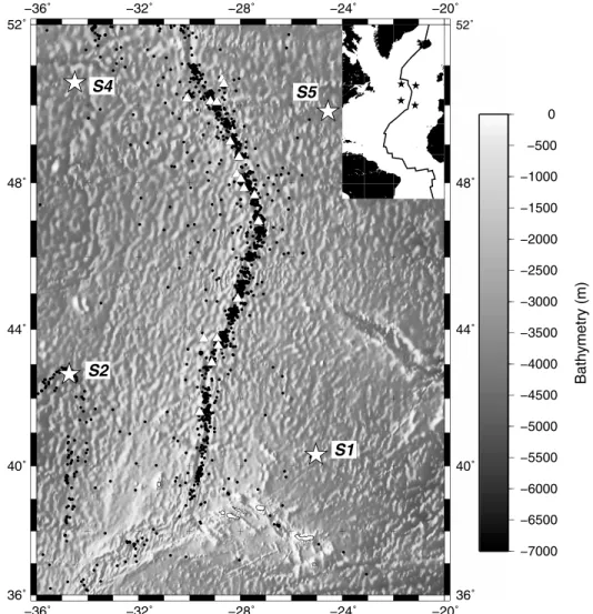
To test the method’s performance, we have used the data acquired during the hydroacoustic experi-ment SIRENA conducted in the North Atlantic from May 2002 to September 2003 [Goslin et al., 2004]. The hydrophone network comprised four instruments, which were installed on the western and eastern sides of an approximately 1000 km long section of the north Mid-Atlantic Ridge (Figure 6). This particular exper-iment was chosen for a verification of the method because its data were already fully analyzed using the conventional approach of visual inspection. As a result, a catalog listing all the seismic events localized from the observed T waves was available. The catalog helped to minimize the amount of time spent on the preparation of the training data set needed for the fitting of the statistical model (section 2.2).
The original sampling frequency of the SIRENA records was 250 Hz. To speed up the calculations, the records were filtered with an antialiasing low-pass filter with a corner frequency of about 40 Hz and then down-sampled to 80 Hz. The low-pass filtering of the original data does not lead to the loss of information since the frequency content of the T waves normally does not extend beyond 20 Hz. With this pretreatment, the first scale of the wavelet transform corresponds to the frequency band located approximately between 20 and 40 Hz (see section 2.1), while the last seventh scale corresponds to a frequency range between
Journal of Geophysical Research: Solid Earth
10.1002/2013JB010936
Figure 6. Bathymetric map of the Mid-Atlantic Ridge section surveyed during the SIRENA experiment. Stars indicate the
hydrophones whose records were used to locate the events denoted by dots. Hydrophones S2 and S5 are in the lower left and upper right corners of the network, respectively. White open triangles give the positions of the epicenters of large magnitude earthquakes listed in the National Earthquake Information Center (NEIC) catalog for the duration of the experiment. The inset gives a global view of the SIRENA network (with hydrophones again indicated by stars).
approximately 0.3 and 0.6 Hz. As can be seen in Figure 3, the seven-scale wavelet transform covers a sufficient number of frequency ranges to exploit the differences in the spectra of the detected signals. We have applied the method to the records of the hydrophones S2 and S5 located at (42.72◦N, 34.72◦W) and (49.86◦N, 24.57◦W), respectively (Figure 6). The analysis covered the time period from 1 June 2002 to 1 May 2003. First, we applied the STA/LTA algorithm, which resulted in a total of 1570 and 1329 signals detected for hydrophones S2 and S5, respectively. In the next step, the types of the detected signals were manually iden-tified in order to produce a training data set. By calculating the expected arrival times of T waves generated by the events listed in the catalog and matching them with the times of the STA/LTA triggers (10∼s long time window centered on the STA/LTA trigger was taken), the vast majority of the detected signals were found to be T waves. Similarly, teleseismic P waves were identified by matching the times of the triggers with the arrival times of the seismic phases predicted for the model IASP91 [Kennett and Engdahl, 1991] for the events listed in the NEIC catalog. Signals whose trigger times were not matched by the predicted arrival times were examined visually. Some of these signals were found to be generated by passing ships. They normally last between 20 and 50 s and were easily identifiable from their spectrograms as can be seen from Figure 2. The last important class of the detected signals contains sounds generated by icebergs [Talandier et al., 2002;
Dziak et al., 2010; Chapp et al., 2005; MacAyeal et al., 2008; Royer et al., 2009]. In general, iceberg-generated
Table 1. Summary of the Detections for Hydrophones S2 and S5
Signal Type Number of Occurrences in S2 Number of Occurrences in S5
P waves 17 22
T waves 1476 1224
Ship generated 14 12
Iceberg generated 63 71
Total 1570 1329
(sometimes weaker) harmonics. An additional unmistakable property of such signals helping in their iden-tification is the temporal variation of the emission frequencies (Figure 2). The rest of the detected signals were T waves whose origin events were not listed in the catalog (i.e., event localization was not possible since generated T waves were detected by fewer than three hydrophones) as well as several Pn waves. It was found that each of the Pn waves was followed by a high-amplitude T wave arriving on average 200 s later. This small time separation suggests that each pair of Pn and T wave signals was produced by the same nearby event. In all cases, the spectral content of Pn and T waves was very similar. This allowed us to con-sider Pn and T waves as signals of the same type for discrimination purposes. This does not impede the future localization of the events, since an identification of a Pn wave would signify a simultaneous identi-fication of a T wave signal following it closely. In the rest of the paper, the term “ensemble of the T waves” includes also Pn wave signals.
Both data sets contained numerous signals due to marine mammal vocalizations. However, these signals have a duration much shorter than the STA window length, such that the STA/LTA ratio never exceeds the trigger threshold. Thus, the data analyses in geophysical and biological domains are conveniently decoupled by the very nature of the corresponding signals.
Although very common in hydroacoustic data, there was only one short period during which air gun signals were observed in our records (of hydrophone S5). Again, because of the short signal duration, none of these few air gun-generated signals were detected by the STA/LTA algorithm.
It should be noted that our STA/LTA parameters were optimal primarily for the detection of seismic signals (T and P waves), for which we wish to develop the automatic identification procedure. Naturally, effective detection of other signal types would require the readjustment of these parameters.
Table 1 provides a summary of the signals detected by each hydrophone.
4. Results
4.1. Evaluation of Predictive Power: Self-Prediction
A usual first step in an automatic classification analysis is the evaluation of the ability of a cross-validated model (which should therefore hold some generality) to repredict the training data set. Being built on the training set, the model is likely to be better at predicting this particular data than any other data. Therefore, the self-prediction results serve as a benchmark of the best possible performance the model can produce when applied to future independent data sets. Using the detected signals presented in Table 1, two separate models were fit to each data set.
4.1.1. Hydrophone S2
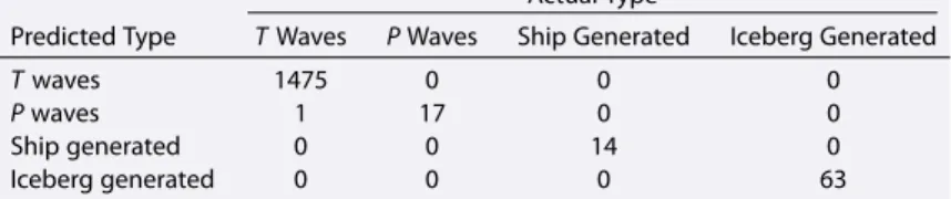
The most discriminating characteristics of the model were scale averages at scales 3, 2, and 4 (these scale averages were present in the binary splits of 30%, 30%, and 23% of trees, respectively). This could be expected from the distribution of scale averages shown in Figures 3 or 4: the signals of all types are well sep-arated at these scales but overlap more at scale 7, for example. A convenient way to present the results of the identification is a confusion matrix (Table 2) which for all signals compares in a single table the actual types (columns) with the predicted ones (rows). In other words, its entries list how many signals of a given type were predicted to be of the same, or of another type. For example, from Table 2 it can be seen that during the self-prediction test one T wave was predicted to be a P wave. When all the signals are identified correctly, only the diagonal elements of the confusion matrix are nonzero. As all but one of the nondiagonal elements in Table 2 equal zero, the results of the self-prediction test for hydrophone S2 are almost perfect. The performance of an identification method can also be described in terms of precision, recall, and F1 score. These quantities summarize the more detailed information provided by the confusion matrix. Precision of
Journal of Geophysical Research: Solid Earth
10.1002/2013JB010936
Table 2. Confusion Matrix of the Self-Prediction Test for the Hydrophone S2 Model
Actual Type
Predicted Type T Waves P Waves Ship Generated Iceberg Generated
T waves 1475 0 0 0
P waves 1 17 0 0
Ship generated 0 0 14 0
Iceberg generated 0 0 0 63
the classifier quantifies how “pure” each predicted category is. It is computed as the number of true pos-itives (i.e., correctly identified signals) divided by the total number of signals predicted in this category. Recall gives the fraction of signals of a given type that the model is able to correctly classify. It is defined as the ratio of the number of the true positives to the total number of signals of this type. In terms of the notation used in Table 3, precision and recall for a given signal type are expressed as TP∕(TP + FP) and TP∕(TP + FN), respectively.
A trade-off usually exists between precision and recall. Quite frequently, when a method correctly identifies all or most of the signals of a given type (very high recall) it also ascribes a substantial number of signals of other types to the same group, thus lowering the precision. Conversely, when the precision is very high, it is often because a method is too restrictive and thus many other signals of the same type are rejected (low recall). The F1 score combines both quantities into a single criterion; the higher the value of F1 score, the better is the performance of the method. The F1 score is defined as follows:
F1 = 2⋅ precision⋅ recall
precision + recall . (3) Table 3 provides a summary of the confusion statistics for the self-prediction test of hydrophone S2. For each identification, the model predicts the probability to be of each of the four types since each “leaf,” or final group, can contain signals of all four types (Figure 5). The signal is identified to be of the type which has highest probability in the group. To check how confident we can be in our classification, we compared the four probabilities for each signal: the higher the probability corresponding to the true type of the signal (as compared to the other three probabilities), the more robust is the identification. Figure 7 confirms that the identification of signals of seismic origin is very robust: the probabilities of being of the correct type are mostly close to one, and the possibility of confusion with other signals is very small (since the probabilities of being of another type are near zero). The same holds for ship- and iceberg-generated signals. Only one
T wave was identified as a P wave. For this signal the probabilities to be a T wave and a P wave are low and
very close, with that for a P wave being slightly higher. This misidentification lowers recall for T waves and precision for P waves. If the objective is to detect as many T waves as possible (i.e., high recall), a solution would be to focus only on the probability pTof being a T wave (discarding the other three probabilities),
set a threshold tT, and consider any signal with pT > tTas a T wave. However, such an increase of the recall
might come at the expense of the decrease of the precision since signals of other types, but with a high enough value of pT, would also be classified as T waves. In the case of hydrophone S2, the probabilities are
different enough that even a relatively low threshold of 0.25 would ensure capturing all T waves with very few false positives. If higher precision in the identification of P waves is important, the solution is to impose a more stringent criterion on the probability pPof being a P wave. In addition to the requirement for pPto be
Table 3. Confusion Statistics of the Self-Prediction Test for the Hydrophone
S2 Modela TP FP FN Precision Recall F1 T waves 1475 0 1 100% 99.9% 99.95% P waves 17 1 0 94.4% 100% 97.12% Ship generated 14 0 0 100% 100% 100% Iceberg generated 63 0 0 100% 100% 100%
aThe abbreviations used are TP = true positives, i.e., correct identifications;
FP = false positives, i.e., incorrect identifications; and FN = false negatives, i.e., false rejections.
Figure 7. Probabilities to be of all four possible types (vertical axis) predicted by the method during the self-prediction test on the training data set of hydrophone
S2. Signals are split in four panels according to their actual type. To facilitate readability, signals in each panel are arranged in such a way that the probability of being of the correct type decreases monotonically (these probabilities are joined by a line). The highest probability among the four possible types is high-lighted by a larger and darker symbol. Thus, a given signal is identified correctly if the symbol corresponding to the signal’s actual type is the largest. The better the method’s performance, the higher is the probability corresponding to the actual type and the lower are the probabilities corresponding to other types. This should hold for as many signals as possible. It can be seen that the method performs very well for the signals of all four types, with the exception of (top) one misidentification of a T wave as a P wave (indicated by a larger triangle and a smaller circle).
the highest of the four probabilities, a threshold tPcan be imposed such that any signal initially classified as a P wave but with pP< tPwould be discarded from the P wave group. Again, too high a threshold might also remove some other P waves. As can be seen from Figure 7, a rather high threshold of 0.75 would eliminate the false positive due to a T wave (indicated by a larger triangle in Figure 7 (top) but also one true P wave (indicated by a triangle with the lowest probability in Figure 7 (bottom left)). These examples illustrate the trade-off between precision and recall. This trade-off has to be determined by the user, depending on the relative importance of detecting absolutely all signals in a given group (high recall) versus avoiding false positives (high precision).
4.1.2. Hydrophone S5
In the case of hydrophone S5, the most discriminating characteristics were similar to hydrophone S2 but in a different order: binary splits based on the scale average values at scales 2, 3, and 4 are present in 37%, 36%, and 12% of the trees. This could also be expected from Figures 3 or 4: for example, signals are better separated at scale 2 for hydrophone S5 than for hydrophone S2. The confusion matrix for the self-prediction of the hydrophone S5 data is presented in Table 4. The self-prediction results are by a tiny margin worse than those for hydrophone S2: three T waves are misidentified as iceberg-generated signals and two ship-generated signals are predicted to be a T wave and a sound emitted by an iceberg. The summary of the confusion statistics of the self-prediction test for hydrophone S5 is presented in Table 5.
4.2. Operational Prediction: Prediction From a Subsample
The self-prediction tests provide a benchmark for the method’s performance. However, for the method to be useful, it should perform well with a statistical model created from a training set which is a small
subsample of the entire data set. The fewer signals are in the training set, the smaller is the amount of human
Table 4. Confusion Matrix of the Self-Prediction Test for the Hydrophone S5 Model
Actual Type
Predicted Type T Waves P Waves Ship Generated Iceberg Generated
T waves 1221 0 1 0
P waves 0 22 0 0
Ship generated 0 0 10 0
Journal of Geophysical Research: Solid Earth
10.1002/2013JB010936
Table 5. Confusion Statistics of the Self-Prediction Test for the Hydrophone
S5 Modela TP FP FN Precision Recall F1 T waves 1221 1 3 99.9% 99.8% 99.85% P waves 22 0 0 100% 100% 100% Ship generated 10 0 2 100% 83.3% 90.89% Iceberg generated 71 4 0 94.7% 100% 97.28%
aThe abbreviations used are TP = true positives, i.e., correct identifications;
FP = false positives, i.e., incorrect identifications; and FN = false negatives, i.e., false rejections.
effort required for their manual identification. Because we observed during the self-prediction test that the discriminating variables involved in the model are not exactly the same for hydrophones S2 and S5, we start by treating them separately before trying to use a single training set applicable to both hydrophones.
4.2.1. Selecting a Representative Data Subset
Our goal is to select a small subset of the signals to fit the model and then use it to predict the types of the remaining signals. The important question is how to choose the signals for the training set. The train-ing set needs to be representative of the entire data set for the model to have acceptable predicttrain-ing power. At the very least, it should contain signals of all types. However, because the vast majority of the signals detected by hydrophones are T waves (Table 1), picking a portion of the signals at random is likely to result in a training set comprising only T waves. Furthermore, even within T waves, considerable variability in the distribution of scale averages exists (see the spread of the distribution of scale averages at scale 4 in Figure 4, for example). Obviously, this variability should also be reflected by the training set. To overcome the lim-itations of the naïve, random choice approach, we have used an unsupervised classification technique to presort the signals in k groups based purely on their characteristics (distribution of scale averages in our case). The technique does not consider any a priori knowledge of their type; in other words, it does not require a training set to function. Its general purpose is to create groups such that signals within each group look similar while signals from different groups look different from each other. As an example, the results of such unsupervised classification of the signals detected by hydrophone S5 are shown in Figure 8. The num-ber of signals in each group is not constrained and therefore varies from one group to another. To build the training set, we randomly picked a fixed number n of signals from each group. This resulted in a training set of k × n signals representing the entire variability of the complete data set (picking the same percentage of signals in each group instead of a fixed number is, in fact, equivalent to randomly drawing the training set which thus will not be representative).
As the types of all signals in our data sets were known, we were able to check whether the preclassifi-cation indeed helps to separate T waves from the much rarer signals (P waves, ship-generated sound, and iceberg-generated sound) and T waves themselves according to their varying properties. The out-come of the unsupervised classification was found not to be very sensitive to the number of groups k. With as few as three groups, most P waves are separated from other signals. With four groups, most of the iceberg-generated signals are separated from T waves. Increasing the number of groups provides further discrimination within T waves. However, creating too many groups might make some of them very small, and extracting n signals from each group would no longer be possible. A good trade-off between discrim-ination and subsetting was found for k = 10 (Figure 8). With the exception of ship-generated signals, whose similarity with T waves prevents the unsupervised classification from separating these two types (see group 4 in Figure 8), iceberg-generated signals and P waves are well separated from T waves (groups 9 and 10, respectively) while remaining groups capture the differences within T waves.
The unsupervised classification algorithm we used was hierarchical clustering with Ward’s aggregation crite-rion [Everitt et al., 2009]. The metric was the Euclidean distance between signals, computed from the “scaled” data set: for each characteristic of the signal the mean is subtracted and the remainder is divided by the variance. Such scaling ensures that we give the same weight to all signal characteristics. Using Ward’s aggre-gation criterion allows focusing on the most marked differences between groups. Using other algorithms such as partition around medoids (k medoids) or partition around means (k means) gave very similar results.
Figure 8. Unsupervised partition of signals detected by hydrophone S5 based on the scale averages through hierarchical clustering. This classification contributes
to separating rare signals from more common T waves, as the vast majority of iceberg-generated signals and P waves are concentrated in groups 9 and 10, respec-tively. It also separates T waves according to the intensity and distribution of scale averages: group 7 could be described as powerful signals with maximum energy in scales 3 and 4, while group 2 would be less powerful signals with maximum of the energy at scales 2 and 3. Similar results were observed for the data set of hydrophone S2. Picking 10 signals in each panel results in a collection of 100 signals more representative of the total variability of the entire data set than picking 100 signals at random.
Finally, one needs to determine what fraction of the entire data set the training should use. A large frac-tion would result in a better predicfrac-tion, because the training set would be more extensive. At the same time, a larger training set would also require more human effort on signal identification. A systematic test of fractions between 6% and 40% showed that a fraction of 10% was already sufficient to provide good iden-tification rates of the seismic signals and that making the training set larger did not significantly improve the predictive power. Proportions smaller than 6% are not acceptable because the corresponding training sets did not comprise all observed signal types, even with the subsampling procedure described above, and were too small to fit enough trees.
4.2.2. Hydrophone S2
Since the signals for the training set are drawn randomly from the full data set (divided beforehand into 10 groups using unsupervised classification as explained in the previous section), the resulting identifications depend on the actual subsample drawn. To assess the effect of randomness, we have computed prediction statistics for 100 independently drawn subsamples. A summary of the results is presented in Table 6. The identification of T and P waves and iceberg-generated signals is quite good, while ship-generated signals are always misclassified. Even with such a small training set, P waves are almost always correctly identi-fied (recall is virtually 100%). Almost all T waves are identiidenti-fied correctly (only five false negatives). Although signals of other types are also identified as T waves (about 1% of all signals identified as T waves are false positives), this result is quite acceptable, at least from the point of view of an operator who will use the pre-dicted T waves to compose a catalog of seismic events. The composition of such a catalog favors rather higher values of recall (i.e., very few missed events) at the expense of precision. False positives will be ruled
Table 6. Confusion Statistics in Case of the Identification of the Signals Detected by
Hydrophone S2a TP FP FN Precision Recall F1 T waves 1471 19 5 98.7% ± 0.2 99.7% ± 0.1 99.2% ± 0.1 P waves 17 2 0 89.2% ± 4.2 99.9% ± 0.8 94.2% ± 2.4 Ship generated 0 0 14 – – – Iceberg generated 58 3 5 95.2% ± 2.8 92.1% ± 4.0 93.5% ± 1.8 aConfusion statistics is obtained from 100 subsamples randomly drawn from 10
groups formed by unsupervised classification procedure. As each signal type is charac-terized by ensembles of true positives (TP), false positives (FP), and false negatives (FN), we report for each ensemble the value of its median as well as the mean and standard deviation of the usual confusion statistics.
Journal of Geophysical Research: Solid Earth
10.1002/2013JB010936
Table 7. Confusion Statistics in Case of the Identification of the Signals Detected by
Hydrophone S5a TP FP FN Precision Recall F1 T waves 1219 10 5 99.0% ± 0.2 99.6% ± 0.2 99.3% ± 0.1 P waves 22 6.5 0 77.0% ± 10.4 99.7% ± 1.4 86.5% ± 6.5 Ship generated 0 0 12 – – – Iceberg generated 67 3 4 94.9% ± 1.8 92.8% ± 5.0 93.7% ± 2.4 aConfusion statistics is obtained from 100 subsamples randomly drawn from 10 groups
formed by unsupervised classification procedure. As each signal type is characterized by ensembles of true positives (TP), false positives (FP), and false negatives (FN), we report for each ensemble the value of its median as well as the mean and standard deviation of the usual confusion statistics.
out during localization of the events and will not present a problem as long as they are not too numerous (which is obviously true in our case of only 19 false positives). As for ship-generated signals, being signif-icantly outnumbered by T waves (group 4 in Figure 8), random picking of these signals when composing the training set is very unlikely. The scarcity or even absence of ship-generated signals in the training sets explains their poor classification in the operational prediction.
4.2.3. Hydrophone S5
Results obtained for hydrophone S5 (Table 7) are very similar to the results for hydrophone S2. Precision of the P wave identification is slightly worse, but the recall is as good as for hydrophone S2. The confusion between T waves and other signals is also similar to that of hydrophone S2.
4.2.4. Hydrophones S2 and S5
When the data of hydrophones S2 and S5 are merged into a single data set, a subsample of 5% gives a very similar performance (Table 8). Only one false negative occurs for P waves. As for T waves, 12 false negatives were found, which nearly amounts to the sum of false negatives for T waves observed for each hydrophone separately. This means that even though the self-prediction tests on each hydrophone suggested a different order of importance of the discriminatory variables, the fact that the same variables were discriminatory is sufficient to enable the construction of a common model for both hydrophones. Note also that in case of the merged set, the human effort required for manual identification of the training set signals (5% of the total of 2899 signals or about 145 signals) represents half of that needed in case when the identification is per-formed separately for each hydrophone (10% for each data set or about 290 signals in total). In other words, the number of signals required to build an adequate training set for the merged data set is approximately the same as that needed for each of the constituting data sets. This suggests that the quality of the identifi-cation depends on how well the training set represents the diversity of shapes of scale average distributions, rather than what fraction of the total number of available signals it contains. This is not surprising: once a distribution of the scale averages of a given shape is present in the training set, adding more signals with the same distribution shape does not bring new information. In our case, it seems that about 145 signals selected after the unsupervised classification were enough to cover most usual distribution shapes shown in Figure 8. A general advice would therefore be to pool as much data as possible into a single data set before performing the classification. The larger total number of signals achieved by pooling data would also allow
Table 8. Confusion Statistics in Case of the Identification of the Signals Detected by
Hydrophones S2 and S5a TP FP FN Precision Recall F1 T waves 2688 31 12 98.8% ± 0.3 99.5% ± 0.2 99.2% ± 0.1 P waves 38 6 1 85.5% ± 8.9 97.2% ± 2.6 90.6% ± 4.8 Ship generated 0 0 26 – – – Iceberg generated 126 9 8 92.8% ± 2.8 92.7% ± 5.3 92.6% ± 2.6 aConfusion statistics is obtained from 100 subsamples, each subsample making 5%
of a data set obtained by joining data sets of both hydrophones and randomly drawn from 10 groups formed by unsupervised classification procedure. As each signal type is characterized by ensembles of true positives (TP), false positives (FP), and false nega-tives (FN), we report for each ensemble the value of its median as well as the mean and standard deviation of the usual confusion statistics.
Table 9. Confusion Statistics in Case of the Identification of the Signals Detected by
Hydrophones S2 and S5 and Training Sets Simulating High Amount of Shipping Noisea
TP FP FN Precision Recall F1
T waves 2687 8.5 13 99.6% ± 0.2 99.5% ± 0.2 99.6% ± 0.1
P waves 38 5 1 85.4% ± 9.6 97.2% ± 2.7 90.5% ± 5.5
Ship generated 23 2 3 91.1% ± 7.3 86.5% ± 7.2 88.4% ± 5.6
Iceberg generated 125 9 9 93.1% ± 2.7 92.9% ± 4.2 92.9% ± 2.0 aConfusion statistics is obtained from 100 subsamples, each subsample making 5% of
a data set obtained by joining data sets of both hydrophones. As in the test presented in Table 8, signals in the subsamples were randomly drawn from 10 groups formed by the unsupervised classification procedure. Then, five randomly chosen signals were replaced by five randomly chosen ship-generated signals. As each signal type is characterized by ensembles of true positives (TP), false positives (FP), and false negatives (FN), we report for each ensemble the value of its median as well as the mean and standard deviation of the usual confusion statistics.
using a larger number of groups k in the unsupervised preclassification, hence refining the different signal categories and possibly isolating and representing particularities of each hydrophone.
In all tests presented so far, none of the ship-generated signals were correctly identified, since their small number and relative resemblance with T waves (Figure 8, group 4) prevented their random pick-ing for trainpick-ing sets. In fact, most of the ship-generated signals were classified as T waves. As long as the number of these few false positives is small, they will not add a significant amount of extra work for an analyst performing event localization from the list of signals identified by the method as T waves. Obvi-ously, data acquired in regions with intense shipping will contain many more ship-generated signals, and subsequently, some of them will be invariably present in the training sets. At the suggestion of the Asso-ciate Editor, we did an additional classification test, in which we forced the inclusion of five randomly drawn ship-generated signals in each training set, thus simulating a situation with heavy shipping. The results are presented in Table 9. Comparison with Table 8 shows that now 23 out of 26 ship-generated signals were cor-rectly identified; as expected, the number of false positives for T waves was significantly reduced (from 31 to 8.5). This last test proves that the GBDT technique is capable of efficiently discriminating ship-generated signals as soon as some information is available in the training set.
4.2.5. Source Level of Completeness
Another way to evaluate the method’s performance and usefulness is to estimate the source level of com-pleteness (SLc) of the event catalog which would be obtained from the T waves identified by the method.
This is possible because a one-to-one correspondence can be established between an identified T wave and an event in the complete catalog (see section 3). For each event, the catalog provides the value of event’s source level (SL) which is a quantity serving as an estimate of the magnitude of a hydroacoustic event, or in other words, the amount of energy released by the earthquake into the water column at the point of seismoacoustic conversion. It is measured in decibels (with respect to micropascal at 1 m) and calculated from the amplitude of a T wave by taking into account losses along the propagation path and instrument response [Dziak, 2001; Bohnenstiehl et al., 2002]. The SLcis the minimum value of the SL at which the
loga-rithm of the cumulative number of events departs from a linear relationship. The SLcis thus similar to the
magnitude of completeness Mccomputed for a seismic catalog by fitting the Gutenberg-Richter law. A lower
SLcvalue corresponds to a more complete catalog. The difference between the SLcobtained from the events
identified by our automatic method and the SLcderived from the complete catalog allows us to compare
the method’s performance with that of a human analyst.
From the complete catalog, the value of SLcwas estimated to be 209 dB [Goslin et al., 2012]. At this level, the
cumulative number of localized events differs from the one predicted from Gutenberg-Richter law by 7.4%. Then, for both hydrophones, the cumulative number of events as a function of the SL was calculated from
T waves identified by the method. The resulting dependencies (one for each of the 100 random realizations
of the training set) were found to be virtually identical within each hydrophone. This is an important result as it further underlines the small influence of the randomness in the choice of the training set on the com-pleteness of the seismic catalog. The performance of the method presented here is therefore representative of what would be observed in a real-world scenario, when only one training set would be drawn at random. This allowed us to obtain an overall cumulative number versus the SL relationship for each hydrophone by
Journal of Geophysical Research: Solid Earth
10.1002/2013JB010936
averaging the curves found for each subsample. Finally, the SLcvalues for each hydrophone were estimated from average curves by finding the SL value at which the difference between the cumulative number and the number predicted by fitting the Gutenberg-Richter law was equal to the percentage value found from the complete catalog, i.e., 7.4%. The SLcvalues thus estimated are 210.9 dB and 211.1 dB for hydrophones
S2 and S5, respectively. These values are extremely close and are different only by about 2 dB from the SLc
estimated from the complete catalog. Thus, the catalog derived from the T waves identified solely by our automatic method would be virtually identical to the one compiled manually.
5. Conclusions
A new method for automatic signal identification is presented. The method utilizes differences in the sta-tistical properties of the spectra of different signal types. Signal detection is performed with the classical STA/LTA algorithm. Information on the signal spectrum is obtained by calculating its wavelet transform, while the identification of detected signals is realized with the GBDT technique. In this technique, a sta-tistical model is first fit to a training set (a small subset of an entire data set) consisting of the signals whose types are known. The derived statistical model is then used to predict the types of the remaining unknown signals.
The method was applied to the 11 month long continuous records of two moored hydrophones which were part of a hydrophone network deployed during the hydroacoustic experiment SIRENA (North Atlantic). The STA/LTA algorithm was first run on data sets of both hydrophones, and the types of all detected signals were manually identified. Both data sets contained signals of four different types: T waves, teleseismic P waves, ship-generated sound, and iceberg-generated sound. The results of the self-prediction tests (identification of the same data used to construct the statistical model) served as a benchmark of the best possible method performance. Using all detected signals as training sets, the self-prediction showed virtually perfect identi-fication for both hydrophones. To simulate a more realistic case of an analysis of a new unknown data set, a small portion of the signals was considered as the training set and then used for the identification of the remaining signals. The difficulty of choosing signals for the training set (which must be representative of the entire data set) was overcome by using an unsupervised classification algorithm which allowed the splitting of the ensemble of the signals into groups based solely on the statistical properties of their spectra. A collec-tion of signals drawn at random from each group formed the desired representative training set. Choosing only 10% of the total number of the signals recorded by each hydrophone was sufficient to achieve high identification rates for the signals of seismic origin (teleseismic P and T waves) which are the signals of the most interest in hydroacoustic experiments. Furthermore, when the signals of both hydrophones were merged, the method provided similar performance with a training set making 5% of the combined data set (approximately the same number of signals used to build training sets for each of the constituting data sets). Additionally, the identification rate of ship- and iceberg-generated signals is comparable to that of seismic signals. In conclusion, our results demonstrate the high potential of the presented automatic signal identifi-cation method, whose appliidentifi-cation is in principle not limited to the analysis of hydrophone data. The method might thus prove useful for other geophysicists working with any large data sets and wishing to automate the preliminary (i.e., signal identification) part of the data analysis.
References
Allen, R. V. (1978), Automatic earthquake recognition and timing from single traces, Bull. Seismol. Soc. Am., 68(5), 1521–1532. Bohnenstiehl, D. R., M. Tolstoy, R. P. Dziak, C. G. Fox, and D. K. Smith (2002), Aftershock sequences in the mid-ocean ridge environment:
An analysis using hydroacoustic data, Tectonophysics, 354(1–2), 49–70, doi:10.1016/S0040-1951(02)00289-5.
Bohnenstiehl, D. R., M. Tolstoy, D. K. Smith, C. G. Fox, and R. P. Dziak (2003), Time-clustering behavior of spreading-center seismicity between 15 and 35◦N on the Mid-Atlantic Ridge: Observations from hydroacoustic monitoring, Phys. Earth Planet. Inter., 138(2), 147–161, doi:10.1016/S0031-9201(03)00113-4.
Bohnenstiehl, D. R., F. Waldhauser, and M. Tolstoy (2008), Frequency-magnitude distribution of microearthquakes beneath the 9◦50’N region of the East Pacific Rise, October 2003 through April 2004, Geochem. Geophys. Geosyst., 9, Q10T03, doi:10.1029/2008GC002128. Breiman, L., J. H. Friedman, R. A. Olshen, and C. J. Stone (1984), Classification and Regression Trees, vol. 1, Wadsworth, Belmont, Calif. Chapp, E., D. R. Bohnenstiehl, and M. Tolstoy (2005), Sound-channel observations of ice-generated tremor in the Indian Ocean, Geochem.
Geophys. Geosyst., 6, Q06003, doi:10.1029/2004GC000889.
Cohen, A., I. Daubechies, and J. Feauveau (1992), Biorthogonal bases of compactly supported wavelets, Commun. Pure Appl. Math., 45, 485–560.
Dai, H., and C. MacBeth (1997), The application of back-propagation neural network to automatic picking seismic arrivals from single-component recordings, J. Geophys. Res., 102(B7), 15,105–15,113, doi:10.1029/97JB00625.
Dziak, R. P. (2001), Empirical relationship of T-wave energy and fault parameters of northeast Pacific Ocean earthquakes, Geophys. Res.
Lett., 28(13), 2537–2540, doi:10.1029/2001GL012939.
Acknowledgments
Alexey Sukhovich received financial support from the CNRS Chair of Excel-lence award. Guust Nolet received financial support from the ERC (advanced grant 226837). The authors would like to thank Maya Tolstoy, Won Sang Lee, an anonymous reviewer, and the Associate Editor for reviewing the paper and providing a number of con-structive comments. The data used in this paper are available from the authors upon request.