HAL Id: hal-01074460
https://hal.archives-ouvertes.fr/hal-01074460
Submitted on 8 Jan 2015
HAL is a multi-disciplinary open access
archive for the deposit and dissemination of sci-entific research documents, whether they are pub-lished or not. The documents may come from teaching and research institutions in France or abroad, or from public or private research centers.
L’archive ouverte pluridisciplinaire HAL, est destinée au dépôt et à la diffusion de documents scientifiques de niveau recherche, publiés ou non, émanant des établissements d’enseignement et de recherche français ou étrangers, des laboratoires publics ou privés.
Distributed under a Creative Commons Attribution - NonCommercial - NoDerivatives| 4.0 International License
Classifier systems evolving multi-agent system with
distributed elitism
Gilles Enee, Cathy Escazut
To cite this version:
Gilles Enee, Cathy Escazut. Classifier systems evolving multi-agent system with distributed elitism. Congress On Evolutionary Computation 1999, Jul 1999, Washington D.C., United States. pp.1740 -1746, �10.1109/CEC.1999.785484�. �hal-01074460�
Classifier Systems
Evolving Multi-Agent System with Distributed Elitism
Gilles ENEE
Laboratoire I3S - Les Algorithmes Bˆatiment Euclide - 2000 Route des Lucioles
Sophia-Antipolis 06410 BIOT, France phone : +33 (0) 4-92-94-27-72
e-mail: [email protected]
Cathy ESCAZUT
Laboratoire I3S - Les Algorithmes Bˆatiment Euclide - 2000 Route des Lucioles
Sophia-Antipolis 06410 BIOT, France phone : +33 (0) 4-92-94-27-74
e-mail: [email protected]
Abstract-Classifier systems are rule-based control systems for the learning of more or less complex tasks. They evolve in an autonomous way through solution without any ex-ternal help. The knowledge base (the population) con-sists of rule sets (the individuals) randomly generated. The population evolves due to the use of a genetic algorithm. Solving complex problems with classifier systems involves problems to be split into simple ones. These simple prob-lems need to evolve through the main complex problem, ’co-evolving’ as agents in a multi-agent system. Two different conceptual approaches are used here. First is
Elitism that is inspired by Darwin, distinct agents evolving
always keeping alive their best members. Second is
Dis-tributed Elitism which is a logical enhancement of Elitism
where agents knowledge is distributed to make the whole evolve through solution. The two concepts have shown in-teresting experimental results but are still very different in use. Mixing them seems to be a fairly good solution.
Keyword list : Genetic Algorithm, Classifier System, Multi-Agent System, Genetics Based Machine Learning, Knowledge Sharing.
1 Introduction
Solving complex problems with classical algorithms has shown its limits. In our work, the solutions space of complex problems is explored thanks to genetic algorithm [Goldberg, 1989]. Genetic algorithms are not dedicated to machine learning. Then [Holland, 1992] has introduced
Clas-sifier Systems which are an extension of genetic algorithm as
it is described in the next sections. These systems are special-ized in learning. But even with these tools, we are obliged to split complex problems into simple ones [Bull, 1995]. These simple problems are considered as agents co-evolving in a multi-agent system. But we still encounter difficulties to an-swer to complex problems due to the actual lack of general conceptual approach. In this paper, we will first describe Pittsburgh-style classifier systems and multi-agent systems. Section 3 will present our experiments. In that section, we will first explain the traffic signal controller we used for the tests, second will be the Elitism experiment, third will be the
Distributed Elitism experiment, fourth will be the mixed one and last we show robustness of the chosen classifier system through three experiments. Finally, last section will attempt to show new conceptual openings.
2 Multi-Agent System
Before explaining what is a multi-agent system we must first describe what a genetic algorithm is.
2.1 Genetic Algorithm in Classifier Systems
Genetic algorithms are usually used for function optimiza-tion. The problem is encoded on a bit ’fragment’ called chromosome referring to DNA. They work on a population of chromosomes called individuals. Genetic algorithms use the implementation of DNA’s manipulators like crossover and mutation on this population. They implement natural selec-tion of good soluselec-tions based upon Darwin’s model. The ini-tial set of chromosomes is randomly iniini-tialized over a ternary alphabet 0, 1, #✁ where ’#’ is a wildcard matching for a 1 or
a 0. Crossover consists in randomly taking two chromosomes (parents) and crossing them at a random position exchanging part of their fragments giving two children. For example, let us describe a crossover between individuals 0011 and 1100. If we suppose that the crossover site is situated on the mid-dle of the chromosome, the two children 0000 and 1111 are obtained.
Mutation consists in changing a bit value into one of the two other possible values of the alphabet. Mutation and crossover are applied with a probability of occurring. Genetic algorithms are also used in machine learning system.
2.2 Pittsburgh-style Classifier Systems
Classifier systems are genetics based machine learning sys-tems. They only use genetic based operators to find problem solution. They are made of sets (individuals) of rules (chro-mosomes), the whole consists in a population. Classifier sys-tems exist in two forms : Michigan-style ones and Pittsburgh-style ones. In the first one, one individual is a single rule, in the second one, one individual is a set of rules. Let us detail Pittsburgh-style classifiers [Smith, 1980], since it is the ap-proach we have chosen. The basic cycle of such a classifier
system is the following one :
Initialize(Pop);
While(conditions not satisfied) {
Evaluate(Pop); GA(Pop); }
The population is a set of individuals, each individual be-ing a set of rules. Rules encode the problem as a production
rule i.e with a condition part and an action part. The final
population should contain many individuals representing the solution to execute the task to be learnt. The evaluation con-sists in steps during which each individual of the population will be evaluated many times to measure its performance to accomplish the asked task. The performance gives a reward to the individual in the form of strength. This strength will be used by the genetic algorithm and is essential to the se-lection. The more there are trials, the more the strength is relevant. Once the evaluation done, individuals need to be evolved. This is done by the genetic algorithm. The highly fit individuals (best strength) should ’reproduce’ each other because the random selection is made following a scheme that favors the more fit members. Then crossover and mu-tation mechanisms are applied to recombine individuals. A new population is thus created, containing a higher propor-tion of the characteristics possessed by the good members of the previous population. Each passing through the loop cor-responds to a generation.
2.3 Multi-agent Classifier System
Complex problems need to be split into simple ones [Bull and Fogarty, 1994], expecting these simple problems might be coordinated to answer the main one. This is what we do in a multi-agent system. An agent, in our work, is a classifier system that must solve a simple problem. Thus a multi-agent system is a system composed of agents (classifier systems) that solve together the complex problem.
3 Experiments
Let us now describe the application of our multi-agent classi-fier system.
3.1 Adaptation to a traffic signal
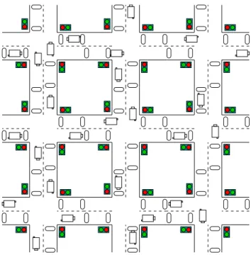
To implement our system, we have chosen the traffic signal controller which is a good example of homo-geneous environment [Bull, Carse and Fogarty, 1995], [Mikami and Kakazu, 1993] and [Mikami and Kakazu, 1994]. This problem has been widely treated in related areas [Escazut and Forgarty, 1997] and [Montana and Czerwinski, 1996]. Each agent manages one junction, the aim is to control a map of crossroads that implies cooperation between junctions.
The grid map we used is a 3✂ 3 one. A junction is made
with four roads at each cardinal point (North, East, South,
Figure 1: The Simulator.
West). Each road has a traffic light which colors are opposed vertically and horizontally. The traffic light is green or red. There is also two sensors giving informations on incoming cars. The nearest one of the traffic light is detecting if a car is waiting at the crossroad, the other one detects a car approach-ing (see figure 1). Cars have a constant speed or are waitapproach-ing for the signal to turn green (no speed), in other words, there is no acceleration. Each road has a traffic flow which is the probability that a car may appear on it. The number of cars by road is limited to 10. The controller shall decide whether the signal must change or not. A cycle is the time between each decision of the controller. Each cycle starts with the execution of the action dictated by the controller. Then, ve-hicles that can move forward, achieve a one-step move. A vehicle that crosses the junction can go straight or turn left or right using a turning probability of 10%. When a car turns, cutting the opposed road, there is no collision. Roads are ’double-sided’. Roads of junctions that are connected to an other junction only receive cars from that neighbour junction i.e. cars cannot be created on that road.
The main problem is to control a 3✂ 3 grid map of
junc-tions. Then according to our choices, we say that the multi-agent system is the map and that an multi-agent is attributed to a junction. Thus we have here nine agents. Now let us see how an agent will rule the junction in our particular case.
There are four input roads per junction and each road has two sensors returning true or false. Thus, the condition part of a rule has two bits by road representing the state of the two sensors on it and a bit to represent the traffic light on the north road that gives the color of other signals. So the condition part of a rule is made of nine bits. The action part consists in changing whether or not the traffic light which is represented
using one bit. For instance, the rule 11 00 11 00 1:1 says that when there is no cars on the East-West roads (xx 00 xx 00 x:x) and there is a North-South important flow (11 xx 11 xx x:x) and when the vertical traffic lights are red (xx xx xx xx 1:x) then the controller must change the state of the traffic lights (xx xx xx xx x:1). Figure 2 represents an individual where A is the Arriving sensor and J the Junction sensor of the indi-cated road. Rule n Rule 1 Rule i
A
J
A
J
A
J
A
J
North Red LightNorth East South West
Action
Figure 2: An Individual.
At each tic (i.e. time interval), a car should advance or wait. A cycle corresponds to 5 tics. Each cycle an individ-ual takes a decision, choosing randomly one rule among the matching rules. Each junction is ruled by an agent also called population. The evaluation of populations is made measuring the performance of all individuals filling it. Each individual✄
is evaluated regarding its performance on its junction. At the end of an evaluation,✄ is given a strength which is the
fluc-tuation between the average delay obtained at the end of the first generation by the whole of the individuals and the one obtained by✄ for the current generation. Strength is given
using this function :
☎✝✆✟✞✝✠☛✡ ☞✍✌✏✎✒✑✓✆✕✔✝✌✗✖✙✘✛✚✢✜✤✣✦✥★✧✪✩✬✫✤✭✮✙✯✱✰✳✲
✎✴✎✵✑✶✆✕✌ ✷✙✑✶✸✺✹✼✻ ✽✾✠☛✎✒✿❀✌ ❁❂✡✼✑✓✎✵✹✝✔✤✑ ✷✙✑✶✸✺✹✼✻❄❃
❅❇❆❉❈❋❊✼●✒❍ ■❑❏▼▲✵❊✝◆P❖✕▲ ◗✦▲✒❘❙◆❯❚
is the mean of the average de-lays the 900 individuals (i.e. 9 junctions of 100 indi-viduals) have obtained at the end of the first generation upon their junction.
❅❲❱❨❳✍❊❩❊❩▲✒❬❭❍ ◗❪▲❩❘❙◆P❚
is the average delay the evaluated in-dividual has obtained at the end of the current genera-tion upon its juncgenera-tion.
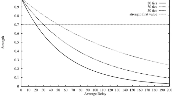
The❆❉❈❋❊✼●✒❍ ■❑❏▼▲✵❊✝◆P❖✕▲ ◗✦▲✒❘❙◆❯❚
is the reference performance for the next generations. Figures 3 shows how an individual will be rewarded when it is evaluated comparing its performance to the mean of the first average delays obtained by the 900 individuals. First generation mean values proposed here are 20, 30 or 50 tics. The starting mean strength is 0.7 for the 900 individuals. We use▲✒❫P❴
function as a delay minimization function. It allows an important enough slope to strengthen or to weaken an evaluated individual. Thus, the more delay decreases through generations, the more strength increases.
0 0.1 0.2 0.3 0.4 0.5 0.6 0.7 0.8 0.9 1 0 10 20 30 40 50 60 70 80 90 100 110 120 130 140 150 160 170 180 190 200 Strength Average Delay
Strength Function of Classifier Systems (Based upon the mean of the first average delays = 20, 30, 50 tics) 20 tics 30 tics 50 tics strength first value
Figure 3: Strength Function.
The parameters of our experiment for the genetic algo-rithm are : ❅ Mutation probability : 0.01 ❅ Crossover probability : 0.6 ❅
Crossover : single point
❅
Selection method : Roulette wheel
A population is composed of 20 individuals, each of them be-ing the concatenation of 15 randomly initialized rules. Indi-viduals performance is averaged after 100 evaluations. Three different flows for roads have been chosen. High flow repre-sents 9 cars per 60 tics, medium flow corresponds to 6 cars per 60 tics, low flow corresponds to 3 cars per 60 tics arriving on a road. The results we present here are averaged over 20 runs with different random seed values. In order to have a global vision of the performance of the whole multi-agent system, the curves we present in the next experiments gives each gen-eration the mean of the average delays for all the 9 agents. In the same way, we always give a reference curve which is the result of an experiment without any enhancement.
3.2 Elitism
Inspired by works made by [De Jong, 1975] on Genetic Al-gorithms, the aim of the Elitism is to keep the best individuals deleting the worst ones in order to strengthen reinforcement.
To implement Elitism, the❵ best individuals of the last
generation are to be placed in the new generation. They re-place the❵ worst individuals. The remaining individuals are
created as usually, i.e applying crossover and mutation oper-ators.
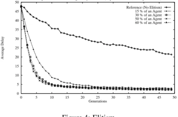
In this experiment, North flow is high, South flow is medium and East-West flows are low. Roads that are con-nected have an empty flow because cars come from the neighbor junctions. We have chosen different percentages of Elitism. So❵ is dependent of this percentage. We have
tested the multi-agent classifier system with different values for ❵ : 3 (15% of the size of an agent, i.e 15% of 20), 6
0 5 10 15 20 25 30 35 40 45 50 0 5 10 15 20 25 30 35 40 45 50 Average Delay Generations
Comparison between average delays : Elitism (Pop 20, Rules 15, 20 Exp, 3x3 Junc) Reference (No Elitism) 15 % of an Agent 30 % of an Agent 50 % of an Agent 60 % of an Agent
Figure 4: Elitism.
to the results obtained with the system without Elitism. Fig-ure 4 shows experiment results.
We can see that the simple evolution (reference) does not learn quickly the solution to the main problem. We notice the quick and relatively efficient convergence of Elitism. Toward generation 10, the 30%, 50% and 60% curves have converged to a stable average delay of about 4.2 tics and then decreased slowly to an average delay of about 1.9 tics at generation 50 for a car to wait before crossing junction. Differences be-tween 30%, 50% and 60% curves are slight. The 15% curve has more difficulties to converge. It seems that a 50% rate of Elitism on population is here the best rate to enhance classi-fier systems convergence. This curve shows a gain of almost 96% on the first average delay. The 60% rate is too high and its curve is higher than 50% one. Now that we have seen the already proved efficiency of Elitism, we should extend that method.
3.3 Distributed Elitism
Pittsburgh-style classifier systems can be enhanced like Michigan-style one with some features. Elitism is a good approach that we can apply to a multi-agent Pittsburgh-style system. In an homogeneous environment, where agents learn locally a similar problem, we should share knowledge. Dis-tributed Elitism consists in exchanging the best individuals between these identical agents, trying to reinforce the whole as quickly as possible, through a pool that will receive for transit those individuals. We conceive Distributed Elitism equally sharing individuals between agents. Distribution is made after the evaluation of whole population :
Initialize(Pop);
While(conditions not satisfied) {
Evaluate(Pop);
Distributed_Elitism(Pop); GA(Pop);
}
The distribution of the best individuals of each agent is made through a pool classifier. This pool is not a classifier system so it does not evolve. The pool is filled with the best
individuals of each agent. To have a better sharing of the pool, the global strength of each agent is used to know how many individuals an agent will pool. The more it has a high strength, the more it will place individuals in the pool :
❛❝❜ ❞✾❡✴❡✵✸❢✑✓✞❨✘❄❞✾❡✴❡✒✸ ☞❣✠✐❤❩✑ ✯✛❥ ☞❧❦☛❁❂✔✤✑✓✆✕✌♥♠ ❥ ☞❧❦☛❁✳✸❢✸❢♠ ❅❇♦q♣ r✙s✝s✝❘❙▲❩t
is the number of individuals pooled.
❅❇r✙s✝s✝❘ ✉★❈❋✈❯▲
is the size of the pool.
❅❇✇①✉
is a function that calculates the Global Strength of an agent or more.
❅❇■❑❖▼▲✒❬❭❍
is the considered agent.
❅❇■②❘✐❘
represents all the agents to get the whole strength of our multi-agent system.
Once the pool is filled with the best individuals of all agents, these individuals have to be distributed only once, replacing the worst individuals of each agent. The redistri-bution is ordered : the worst agents take the best individuals from the pool classifier and the best agents take the ’worst of the best’ individuals from the pool. To know how many indi-viduals will be taken by an agent, we use also an equal share method based upon the strength where the worst the strength is, the greatest the number of taken individuals is :
❛✱❜ ③❂✹✤④P✑✓✆✱✘ ❞✾❡✵❡✵✸ ☞⑤✠✐❤❩✑ ✯ ❦ ❥ ☞❧❦☛❁⑥✸❢✸⑦♠❣⑧ ❥ ☞❧❦☛❁❂✔✤✑✓✆✕✌♥♠✗♠ ❥ ☞❧❦☛❁✳✸✺✸⑦♠ ✯ ❦☛❛✱❜ ❁✬✔✤✑✶✆✕✌✗✿★⑧⑩⑨✶♠ ❅❇♦q♣ ❶②◆▼❷✟▲✵❬
is the number of individuals taken from the pool.
❅❇♦q♣ ■❑❖▼▲✒❬❭❍♥●
is the number of agents of our multi-agent system.
In this experiment, North flow is high, South flow is medium and East-West flows are low. Roads that are con-nected have an empty flow because cars come from the neigh-bor junctions. We compare an alone evolution (reference) and different percentages of the whole population using dis-tributed elitism. The different sizes of the pool, that reflect these percentages, are : 27 (15% the whole population, i.e 3✂ 3✂ 20), 54 (30%) and 90 (50%). Figure 5 shows the
av-erage delays that cars wait on the map to cross junctions. Distributed Elitism gives good results indicating that each junction is efficient and that the whole map is also very ef-ficient at the end of the learning. Toward generation 15, the 3 curves have converged to a stable average delay of about 3 tics and converge slowly to an average delay of 1.1 at gen-eration 50. The best curve is 30% of Distributed Elitism. In term of convergence, it is more efficient than simple Elitism. The gain is about 98% on the first average delay. But it needs 3 generations more to converge to less than 4.2 tics. So why should we not mix the both methods ?
0 5 10 15 20 25 30 35 40 45 50 0 5 10 15 20 25 30 35 40 45 50 Average Delay Generations
Comparison between average delays : Distributed Elitism (Pop 20, Rules 15, 20 Exp, 3x3 Junc) Reference (No Elitism nor Distributed Elitism)
15 % of Population 30 % of Population 50 % of Population
Figure 5: Distributed Elitism.
3.4 Mixed experiment
The efficiency of both methods in their domain have been shown (quick convergence for Elitism and better convergence for Distributed Elitism). We have made a last experiment to see if combining these two methods can more improve the results.
The implementation of the combined methods is simple because Elitism and Distributed Elitism are separated in the algorithm :
Initialize(Pop);
While(conditions not satisfied) {
Evaluate(Pop);
Distributed_Elitism(Pop); GA(Pop); /* Elitism */ }
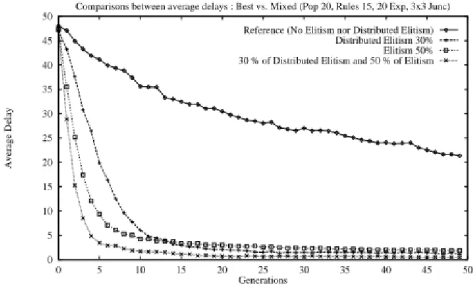
Thus in this experiment, Elitism is performed within each independent agent, and Distributed Elitism is applied be-tween all the agents of the system. So the mechanism favor-ing the best individual is applied at both levels of our multi-agent system. The reference curve used in this experiment is
0 5 10 15 20 25 30 35 40 45 50 0 5 10 15 20 25 30 35 40 45 50 Average Delay Generations
Comparisons between average delays : Best vs. Mixed (Pop 20, Rules 15, 20 Exp, 3x3 Junc) Reference (No Elitism nor Distributed Elitism)
Distributed Elitism 30% Elitism 50% 30 % of Distributed Elitism and 50 % of Elitism
Figure 6: Mixed experiment.
free of any form of elitism. Figure 6 also represents the best Elitism curve (50% of the population of an agent) and the best Distributed Elitism curve (30% of the whole population). The fourth curve displays the average delay vs. the generations for
the system using both Elitism at 50% and Distributed Elitism at a 30% rate.
Results are impressive because we should think that fur-ther gain was nearly impossible. On the fifth generation, av-erage delay is about 3.4 tics, better than the best Elitism. And as final result at generation 50, we have an average delay of 0.47 tic. It is a gain of more than 99% from the first aver-age delay. To figure out this results and to test robustness, we have made three more experiments. Traffic flows on each roads are changed at regular intervals to verify that there is no convergence toward a local optimum and that our mixed solution is a good one.
3.5 Changing flow : Robustness
To test the robustness of our multi-agent classifier systems us-ing the mixed solution, we have done two more experiments during which flows change every 10 generations. In the first test, we will show how the system reacts when faced to a low traffic progressively becoming a very high one. The second experiment is the opposite : the system has to learn how to manage with a very high traffic progressively becoming a low one. The notion of very high flow is represented by a proba-bility of 0.5 for a car to appear on a road at each tic. In other words, with this probability there is every expectation that 30 cars will arrive in 60 tics. On both experiments, flows are randomly set for the ten last generations, i.e. from generation 40 to 50.
The aim of the first experiment is to show that incremental difficulty is not too tough to handle. At the beginning, all incoming flows are low, then they increase to very high :
❅
from generation 0 to 9 flows are low ones
❅
from generation 10 to 19 flows are medium ones
❅
from generation 20 to 29 flows are high ones
❅
from generation 30 to 39 flows are very high ones. Figure 7 represents the reference curve with no Elitism nor Distributed Elitism, and the mixed solution one. The refer-ence experiment seems to have no problems with the chang-ing flows. But the global behavior of the system is not suit-able since at generation 50 the delay is about 20. Considering the mixed solution test, we can notice that at each change of flow the system has to recover from the new flow diffi-culty. But in all cases, it has the expected behavior since it converges quickly even with a sharp difficulty at generation 30 when flows become very high ones. Each 10 generations, production rules that are needed to handle a harder problem are available in the population and are quickly used to lower the average delay. Then, random flows present no difficulties at all to the system, since all cases have already been learnt. Thus, we can say the population keeps enough diversity in order to ensure the robustness of the system.
Let us now detail the second experiment. Here, the system has to learn how to manage with very high flows progres-sively becoming low ones. Figure 8 represents the reference
0 10 20 30 40 50 60 70 0 5 10 15 20 25 30 35 40 45 50 Average Delay Generations
Comparisons between average delays : Changing traffic flow => Easy to Jam (Pop 20, Rules 15, 20 Exp, 3x3 Junc) Reference (No Elitism nor Distributed Elitism) 30 % of Distributed Elitism and 50 % of Elitism
Figure 7: Changing flow from easy to very high.
plot with no Elitism nor Distributed Elitism, and the mixed solution one. We can notice that with this test, the reference system has more difficulties to manage the changing of flows that in the previous experiment. But globally, the average delay is the same (about 20). But, considering the mixed so-lution plot, it is very impressive to see that when the difficulty is higher, the system learns even faster to handle the map of junctions. With a difficulty lowering each 10 generations, it is able to handle at a very good rate the average delay. We can deduce from this experiment that rules needed to handle easier flow problems are contained in the population of the harder one. 5 10 15 20 25 30 35 40 45 50 55 60 0 5 10 15 20 25 30 35 40 45 50 Average Delay Generations
Comparisons between average delays : Changing traffic flow (Pop 20, Rules 15, 20 Exp, 3x3 Junc) Reference (No Elitism nor Distributed Elitism) 30 % of Distributed Elitism and 50 % of Elitism Jam
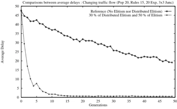
Figure 8: Changing flow from very high to easy. A third experiment has been done : during 50 genera-tions, flows are randomly set and change every 5 generations. Experiment is shown on figure 9. Reference curve uses no Elitism nor Distributed Elitism. It converges slowly as before toward an average delay of 20 encountering slight difficulties each 5 generations. Mixed solution curve learns quickly with a little stop on generation 5 at the first changing flow. This test , we noticed that our system is robust since the average delay is about 0.57 tics at the end of the experiment. After gener-ation 15, when the classifier system has learnt, the varigener-ation of the average delay is only of 0.2 tics each 5 generations while flows change. Those experiments have shown the good reactivity of the classifier system using a mixed Distributed
Elitism and Elitism solution : Robustness is shown.
0 5 10 15 20 25 30 35 40 45 50 0 5 10 15 20 25 30 35 40 45 50 Average Delay Generations
Comparisons between average delays : Changing traffic flow (Pop 20, Rules 15, 20 Exp, 3x3 Junc) Reference (No Elitism nor Distributed Elitism) 30 % of Distributed Elitism and 50 % of Elitism
Figure 9: Changing flow each five generations.
4 Conclusion and further works
This work on multi-agent classifier systems has shown that simplest solutions can be good ones. There is a lot of work to do after this, because generalization of classifiers is far away. We think that there is a way to explore in order to extend conceptual approaches of complex problems to solve them with classifier systems.
It seems that in an homogeneous environment, Distributed Elitism mixed with Elitism is both efficient and robust, now we shall integrate it to classifier systems for learning in such an environment. We shall use a classifier system to rule per-centages of Distributed Elitism and Elitism. That classifier will allow to set rates without knowledge of the best ones for the problem it will handle.
Heterogeneous systems are not as easy to generalize be-cause agents have different goals to achieve, but they are cor-related to solve a single complex problem. Sensors of agents are different and indicate different measures that pooled to-gether and evaluated, give an answer to the problem. These systems need to exchange information between agents intro-ducing the notion of communication and language. They can-not exchange individuals as in an homogeneous environment, disabling the Elitism solution as we present it. Evolution as Artificial-Life of such a communication is a big interest point. Pitssburgh-style classifier systems are interesting and efficient but they need ’evolutions’ as Michigan-style classi-fier systems did. Putting them in an heterogeneous situation and studying their comportment while communicating should be a good answer to rule more and more complex problems.
References
[Bull, 1995] Bull, L. (1995). Artificial Symbiology: Evolu-tion in cooperative multi-agent environments. Ph.D. The-sis , University of the West of England, Bristol.
[Bull, Carse and Fogarty, 1995] Bull, L. Carse, B. and Foga-rty, T.C. (1995).Evolving Multi-Agent Systems. In Genetic
Algorithms in Engineering and Computer Science, Periaux
J. and Winter G., editors.
[Bull and Fogarty, 1994] Bull, L. and Fogarty, T.C. (1994). Evolving cooperative communicating classifier systems. In Sebald, A. V. and Fogel, L. J., editors, Proceedings of
the Third Annual Conference on Evolutionnary Program-ming, pages 308-315.
[De Jong, 1975] De Jong, K.A. (1975). An analysis of the behavior of a class of genetic adaptive systems. (Doc-toral dissertation, University of Michigan). Dissertation
Abstracts International 36(10), 5140B. (University
Micro-films No. 76-9381).
[Escazut and Forgarty, 1997] Escazut, C. and Fogarty, T.C. (1997). Coevolving Classifier Systems to Control Traffic
Signals. In “late breaking papers book”. Genetic
Program-ming 1997 Conference, Koza, John R. (editor).
[Goldberg, 1989] Goldberg, D.E. (1989). Genetic
algo-rithms in search, optimization, and machine learning.
Reading, MA: Addison - Wesley.
[Holland, 1992] Holland, J.H. (1992). Adaptation in Natural
and Artificial Systems. The MIT Press, Cambridge,
Mas-sachusetts.
[Mikami and Kakazu, 1993] Mikami, S. and Kakazu, K. (1993). Self-organized control of traffic signals through genetic reinforcement learning. In Proceedings of the
IEEE Intelligent Vehicles Symposium, pages 113-118.
[Mikami and Kakazu, 1994] Mikami, S. and Kakazu, K. (1994). Genetic reinforcement learning for cooperative traffic signal control. In Proceedings of the IEEE World
Congress on Computational Intelligence, pages 223-229.
[Montana and Czerwinski, 1996] Montana, D. J. and Czer-winski, S. (1996). Evolving control laws for a network of traffic signals. In Koza, J. R., Goldberg, D. E., Fogel, D. B., and Riolo, R. L., editors, Genetic Programming 1996:
Proceedings of the First Annual Conference, pages
333-338. The MIT Press.
[Smith, 1980] Smith, S. (1980). A learning system based on