My teamis in contention? Nice, I go to the stadium! Competitive intensity in the French football Ligue 1

(1)

HAL Id: halshs-00874479

https://halshs.archives-ouvertes.fr/halshs-00874479

Submitted on 7 Apr 2020

HAL is a multi-disciplinary open access archive for the deposit and dissemination of sci-entific research documents, whether they are pub-lished or not. The documents may come from teaching and research institutions in France or abroad, or from public or private research centers.

L’archive ouverte pluridisciplinaire HAL, est destinée au dépôt et à la diffusion de documents scientifiques de niveau recherche, publiés ou non, émanant des établissements d’enseignement et de recherche français ou étrangers, des laboratoires publics ou privés.

Wladimir Andreff, Nicolas Scelles, Christophe Durand, Liliane Bonnal, Daniel

Goyeau

To cite this version:

Wladimir Andreff, Nicolas Scelles, Christophe Durand, Liliane Bonnal, Daniel Goyeau. My teamis in contention? Nice, I go to the stadium! Competitive intensity in the French football Ligue 1. Economics Bulletin, Economics Bulletin, 2013, 33 (3), pp.2365-2378. �halshs-00874479�

(2)

(3)

(4)

1. Introduction

In professional sports economics, the concept of competitive intensity was proposed by Kringstad and Gerrard (2004, 2005) and corresponds to uncertainty of outcome in connection with sporting stakes. In a recent paper, Scelles, Durand, Bonnal, Goyeau and Andreff (2013) investigated the determinants of attendance at French football Ligue 1 matches over the period 2008-2011 and incorporated competitive intensity measured by the points difference for the home team with the closer competitor with a different situation. More precisely, they searched to observe if, between competitive balance (points difference between the two teams before the match) and intensity, one of the two concepts is more relevant in explaining attendance. They found that the effect of competitive balance is not significant but that for competitive intensity is significantly positive.

The aim of this article is to extend this study by envisaging the optimal match temporal horizon for a change in the standing for the home team so that spectators keep their interest. The knowledge of such a match temporal horizon is of prime importance for sports leagues organizers since it gives indications about the optimal number of sporting stakes so that all the teams are in contention (the less important is the match temporal horizon, the more numerous must be the sporting stakes) and, consequently, about the optimal format of the contest.

In this paper, competitive intensity is not any more measured as in Scelles et al. (2013) by the points difference for the home team with the closer competitor with a different situation but by dummies that are function of the points difference for the home team before a match in relation to ranks with sporting stakes. We want to answer the following question: what is the most relevant match temporal horizon for which spectators consider there is uncertainty of outcome? Besides, in Ligue 1, the fifth and sixth ranks are potentially qualifying ranks for the Europa League and become definitely qualified or not qualified ranks according to progress in the two French cups, for which the outcomes are known in the last part of the season. It explains that competitive intensity is measured both with only sure ranks and with sure and potential ranks.

The article is structured as follows. In Section 2, we define the concept of competitive intensity. In Section 3, we describe the organizational and financial structure of Ligue 1, which has implications for competitive intensity measuring and econometric modelling. In Section 4, we outline the model specification for Ligue 1 attendance. In Section 5, empirical results obtained for the 2008-2011 period are reported (1135 observations1). In Section 6, we discuss these results, deal with their implications and envisage avenues. In Section 7, we conclude our study.

2. The concept of competitive intensity

Competitive intensity was proposed by Kringstad and Gerrard (2004, 2005). According to them, apart from the degree of equality between team playing strengths (concept of competitive balance which is currently well documented: Kesenne, 2000; Szymanski, 2001, 2003; Humphreys, 2002; Zimbalist, 2002; Fort and Maxcy, 2003; Groot, 2008; Andreff, 2009; Lee, 2010; Gayant and Le Pape, 2012), audiences are also interested in the prizes that may be distributed in the league (Kringstad and Gerrard, 2007). Consequently, competitive intensity relates to different stakes: qualification in European competitions, relegation in inferior divisions in European leagues or playoff selections in both American and European leagues. Kringstad and Gerrard (2007) select two different indicators depending on whether the leagues are North American (closed) or European (open). For the American leagues,

1_{There are 380 matches during each season. Five matches are excluded from the analysis because they have} been played in camera or in another stadium than the usual one.

(5)

Kringstad and Gerrard use the classic Herfindahl index to analyse the distribution between the participants in playoffs. For the five European football major leagues, Kringstad and Gerrard chose the relegation rate for the teams recently promoted. Consequently, Kringstad and Gerrard rely on original measures with regard to the pre-existent ones by privileging the access to key places: qualification for playoffs or relegation.

Nevertheless, there is a limit in that the analysis does not inform about championship progress, game week after game week. However, it is possible that, using the competitive intensity principle of Kringstad and Gerrard, measures can be proposed that integrate both uncertainty of outcome and sports stakes in a dynamic perspective during one season. In any case, we think that competitive balance represents equilibrium between teams whereas competitive intensity depends on uncertainty of outcome in relation to sporting stakes.

3. The organizational and financial structure of Ligue 1 3.1. Organizational structure

The French football Ligue 1 is recognized as one of the five major European leagues, along with the English Premier League, German Bundesliga 1, Italian Serie A and Spanish Liga 1. It is a championship organized by the French professional football league (Ligue de Football Professionnel, LFP). The competition involves 20 teams and starts in late July or early August to conclude in middle or late May. Each team plays every other team, both home and away, so that there are 38 game weeks and the first classified team is champion (no playoffs). Two characteristics condition sporting stakes and thus teams situations in the standing: the existence of continental competitions and relegations. In Europe, there are two continental competitions: the UEFA (Union of European Football Associations) Champions League, and the Europa League the former being the most prestigious and lucrative. In Ligue 1 as for other European national leagues, the qualification of a team in European competitions depends on its standing:

- the first two are qualified for the next Champions League without participating in the preliminary round;

- the third is qualified for the Champions League preliminary round with the risk of being eliminated in this round and replaced in the Europa League;

- the fourth is qualified in the Europa League.

The fifth and sixth can also be qualified in the Europa League according to results of the two French cups: “La Coupe de France” and “La Coupe de la Ligue”. “La Coupe de la Ligue” concerns only professional clubs whereas “La Coupe de France” involves both professional and amateur clubs. Their winners are qualified for the Europa League. If a winning cup is part of the four first ranks in Ligue 1, the fifth is qualified for the Europa League; if the two French cup winner(s) is(are) part of the four first ranks in Ligue 1, then both the fifth and sixth are qualified for the Europa League. Consequently, the fifth and sixth ranks are potentially qualifying ranks (rather than with sure qualifying ranks) and become definitely qualified or not qualified ranks according to progress in the two French cups, for which the outcomes are known in the last part of the season. This distinction between sure and potential qualifying ranks is of prime importance. We test our attendance equation both for uncertainty of outcome in relation to sure ranks and to sure AND potential ranks in the empirical analysis. For relegations, they concern the three last classified teams. Their existence creates sporting stakes at the bottom of the standing, contrary to American leagues.

(6)

3.2. Financial structure

In 2010-2011, the aggregate turnover without players transfer fees in Ligue 1 was M€1,040 (an average of M€52 by team), similar to amounts in the 2008-2009 and 2009-2010 seasons (see Table 1). Television rights constituted more than half the turnover without players transfer fees. Contrary to American leagues where there are both national and local television rights, Ligue 1 rights are only national for the teams which do not participate in European competitions, and are both national and continental for the others. National television rights are not shared in an egalitarian way (50% versus 30% on sports criteria and 20% on broadcasting criteria with an exponential scale on these criteria).

Table 1. Financial data in the French football Ligue 1 over the period 2008-2011 (amounts in K€)

2008-2009 2009-2010 2010-2011 Turnover without players transfer fees 1 047 833 1 071 603 1 040 480

TV rights 575 673 55% 606 724 57% 607 485 58% Sponsorship and advertising 188 266 18% 177 583 17% 178 716 17% Gate income 150 377 14% 138 157 13% 131 487 13% Other income (essentially merchandising) 133 517 13% 149 139 14% 122 792 12% Salaries expenses 721 581 69% 777 842 73% 776 706 75%

Sources: LFP-DNCG reports (DNCG is Direction Nationale du Contrôle de Gestion, the authority asked to check the clubs accounts)

4. Model specification

We specify and estimate a fairly standard demand equation distinguishing, among the explanatory factors that have an effect on attendance, the following groups of variables: socioeconomic variables, variables proxying the expected quality of the match, those capturing incentives for attending a match, the “season effect” (since there are three seasons) and variables measuring competitive balance and intensity.

We selected a log-linear specification for the demand in football that we write as follows: ATTijt = β0 + βXXi + βZZij + βWWit + βKKjt + βLLijt +εijt (1) where ATTijtis the log-attendance for the match between the home team i and the away team j during the season t, β0 an intercept term, βX the coefficients of explanatory variables Xiwhich depend only on the home team i, βZ the coefficient of the explanatory variable Zij which depends on the home team i and the away team j, βW the coefficients of explanatory variables Wit which depend on the home team i and the season t, βK the coefficients of explanatory variables Kjt which depend on the away team j and the season t, βL the coefficients of explanatory variables Lijt which depend on the match between the home team i and the away team j during the season t and ε a stochastic error term.

Among Xi, we have the home team log-population, the home team log-per capita income per hour, the home team young people percentage, a dummy that is 1 if there is (are) (a) rugby club(s) in the home team area and a dummy that is 1 if the home team waits for a new

stadium.

Zijcorresponds to a dummy that is 1 if the match is a geographical derby.

Among Wit, we have the log-budget for the home team, a dummy that is 1 if the home team has

hooliganism problems (it concerns Paris Saint-Germain) and a dummy that is 1 if the home team was in Ligue 2 during the previous season (promotion effect home).

Among Kjt, we have the log-budget for the away team anda dummy that is 1 if the away team was in Ligue 2 during the previous season (promotion effect away).

(7)

Among Lijt, we have the home team current-month unemployment rate, the standing for the

home team, the standing for the away team, the average number of goals scored by the home team at home, the game week, its square, a dummy that is 1 for matches played during the

week, a dummy that is 1 for matches played on Saturday at 7 pm, a dummy that is 1 for matches played on Saturday at 9 pm, a dummy that is 1 for matches played on Sunday at 5 pm (matches played on Sunday at 9 pm arethe reference and not integrated in the equation),

2009-2010 a dummy that is 1 if the match took place during the season 2009-2010, 2010-2011 a

dummy that is 1 if the match took place during the season 2010-2011 (the season 2008-2009 is the reference and not integrated in the equation), competitive balance measured by the points difference between the two teams in the standing and competitive intensity measured by dummies that are function of the points difference with the closer competitor with a different situation (uncertainty of outcome in relation to sporting stakes; 1 if points difference does not exceed a given value, 0 otherwise).

For competitive intensity, eight match temporal horizons are chosen: the points difference makes possible a change in the standing during the next match, the two next matches… until the eight next matches. Dummies are the same for the temporal horizon of the nine next matches than for the eight next matches. Besides, competitive intensity is measured both with sure ranks only and sure and potential ranks. From the five next matches, dummies are the same both with sure ranks only and sure and potential ranks. We expect a positive effect of competitive intensity dummies (the smaller the difference, the higher the uncertainty of outcome).

The basic data set comes from the French football league (LFP). The sources2 and the descriptive statistics of the variables are presented in Table 2.

Table 2. Descriptive statistics and sources

Mean SD Source

Attendance1 20 290.28 11 402.10 LFP (http://lfp.fr/)

Home team population1 1 184 588.33 2 473 448.27 SPLAF (http://splaf.free.fr/) Home team per capita income per hour1 12.75 1.34 INSEE

(http://insee.fr/fr/default.asp) Home team current-month unemployment rate 0.06 0.01

Gouvernemental Web Site (http://www.travail-emploi-sante.gouv.fr/)

Home team young people percentage 0.31 0.03 INSEE Budget for the home team1 51.92 34.72 France Football

(http://www.francefootball.fr/) Budget for the away team1 51.77 34.52

Standing for the home team 10.73 5.69

LFP Standing for the away team 10.32 5.67 Average number of goals for the home team at home 1.33 0.54

Game week 19.61 10.97

(Game week)² 504.88 441.74

The match played during the week 0.10 0.29 The match played on Saturday at 7 pm 0.54 0.50 The match played on Saturday at 9 pm 0.08 0.27 The math played Sunday at 5 pm 0.19 0.40 The match played Sunday at 9 pm 0.09 0.29

The match is a geographical derby 0.07 0.26 SPLAF There is a rugby club in the home team area 0.13 0.34

Wikipedia

(http://www.wikipedia.org/) The home team has hooliganism problems 0.02 0.13

The home team waits a new stadium 0.30 0.46 The home team was in Ligue 2 during the previous

season 0.15 0.36

LFP The away team was in Ligue 2 during the previous

season 0.15 0.36

2008-2009 0.33 0.47

2

(8)

2009-2010 0.33 0.47

2010-2011 0.33 0.47

Competitive balance 8.26 8.07 Competitive intensity for the next match with only sure

ranks 0.63 0.48

Competitive intensity for the next match with sure and

potential ranks 0.67 0.47 Competitive intensity for the two next matches with only

sure ranks 0.8 0.4

Competitive intensity for the two next matches with sure

and potential ranks 0.83 0.37 Competitive intensity for the three next matches with

only sure ranks 0.896 0.304 Competitive intensity for the three next matches with

sure and potential ranks 0.902 0.297 Competitive intensity for the four next matches with

only sure ranks 0.933 0.250 Competitive intensity for the four next matches with

sure and potential ranks 0.936 0.245 Competitive intensity for the five next matches 0.959 0.199 Competitive intensity for the six next matches 0.963 0.189 Competitive intensity for the seven next matches 0.964 0.187 Competitive intensity for the eight next matches 0.965 0.184

1

These variables are expressed in real terms and not in log terms.

5. Empirical results

We estimated several versions of our equation, using 1135 observations corresponding to 1135 matches that took place in the French football Ligue 1 during the 2008-2011 period (five excluded matches, see Footnote 1). We want to answer the two following questions:

- Does a more relevant temporal horizon exist to consider whether there is uncertainty of outcome in relation to sporting stakes?

- Should only sure or sure AND potential ranks be taken into account?

In a first time, we estimated twelve versions of our equation, eight for the four first temporal horizons – four for only sure ranks and four for sure and potential ranks – and four for the four last temporal horizons. The results are reported in Tables 3, 4 and 5. For all the models, we expected a positive impact of uncertainty of outcome measured through a horizon of matches. The results are based on ordinary least squares with White (1980) standard errors robust to heteroscedasticity.

We only concentrate on competitive intensity in our comments of results. Uncertainty of outcome is significant at the 1% level with all the temporal horizons from three next matches (and both with only sure ranks and with sure and potential ranks for three and four next matches). If we consider the models with only sure ranks, uncertainty of outcome is significant only at the 10% level for the horizons of one and two next matches. If we consider the models with sure and potential ranks, uncertainty of outcome is significant at the 5% level for the horizon of one match and at the 1% level for the horizon of the two next matches. Consequently, three next matches are the weakest temporal horizon for which uncertainty of outcome is significant at least at the 5% level both with only sure ranks and with sure and potential ranks. According to the previous elements, the three next matches could seem a better horizon than one or two next matches to consider whether there is uncertainty of outcome from the spectator point of view. Nevertheless, all the measures of outcome of uncertainty are significant at least at the 5% level with sure and potential ranks. Besides, is the temporal horizon of three matches (and not three next matches anymore, that is to say a reversal is possible in three matches and not before) more significant than one and two matches (and not two next matches anymore) if these three variables and the five others that have been envisaged (from four to eight matches) are simultaneously incorporated?

(9)

Table 3. Estimates of the attendance equation with only sure ranks for the four first temporal horizons

Model 1 Model 2 Model 3 Model 4

Coeff p-value Coeff p-value Coeff p-value Coeff p-value Home team log-population 0.2185 <0.0001 0.2191 <0.0001 0.2216 <0.0001 0.2233 <0.0001 Home team log-per capita

income per hour -2.0937 0.0030 -2.1062 <0.0001 -2.1006 <0.0001 -2.1057 <0.0001 Home team current-month

unemployment rate 3.1220 <0.0001 2.6797 0.0001 2.6808 0.0001 2.6411 0.0002 Home team young people

percentage 0.8451 <0.0001 0.8515 0.0028 0.8423 0.0030 0.8365 0.0033 Log-budget for the home

team 0.7472 <0.0001 0.7577 <0.0001 0.7545 <0.0001 0.7531 <0.0001 Log-budget for the away

team 0.1662 <0.0001 0.1716 <0.0001 0.1712 <0.0001 0.1691 <0.0001 Standing for the home team -0.0069 <0.0001 -0.0070 <0.0001 -0.0066 <0.0001 -0.0067 <0.0001 Standing for the away team -0.0023 0.0402 -0.0022 0.0467 -0.0022 0.0445 -0.0024 0.0339 Average number of goals

for the home team at home -0.0051 0.6858 -0.0045 0.7231 -0.0037 0.7713 -0.0047 0.7106 Game week -0.0107 <0.0001 -0.0115 <0.0001 -0.0124 <0.0001 -0.0130 <0.0001 (Game week)² 0.0003 <0.0001 0.0003 <0.0001 0.0004 <0.0001 0.0004 <0.0001 The match played during

the week -0.0309 0.2415 -0.0327 0.2181 -0.0349 0.1875 -0.0362 0.1687 The match played on

Saturday at 7 pm 0.0019 0.9363 0.0033 0.8915 0.0017 0.9422 -0.0007 0.9761 The match played on

Saturday at 9 pm 0.0048 0.8653 0.0064 0.8195 0.0046 0.8686 0.0047 0.8651 The match played Sunday at

5 pm -0.0259 0.3030 -0.0252 0.3174 -0.0280 0.2637 -0.0301 0.2272 The match played Sunday at

9 pm ref. ref. ref. ref.

The match is a

geographical derby 0.1217 <0.0001 0.1204 <0.0001 0.1195 <0.0001 0.1180 <0.0001 There is a rugby club in the

home team area -0.0081 0.7908 0.0018 0.9518 -0.0001 0.9999 -0.0001 0.9993 The home team has

hooliganism problems -0.1961 <0.0001 -0.2099 <0.0001 -0.2153 <0.0001 -0.2197 <0.0001 The home team waits a new

stadium -0.4374 <0.0001 -0.4393 <0.0001 -0.4401 <0.0001 -0.4416 <0.0001 The home team was in

Ligue 2 during the previous season

0.2274 <0.0001 0.2393 <0.0001 0.2405 <0.0001 0.2373 <0.0001 The away team was in

0.0481 0.0066 0.0652 0.0003 0.0659 0.0002 0.0645 0.0003

2008-2009 ref. ref. ref. ref.

2009-2010 -0.1835 <0.0001 -0.1797 <0.0001 -0.1736 <0.0001 -0.1726 <0.0001 2010-2011 -0.2309 <0.0001 -0.2250 <0.0001 -0.2222 <0.0001 -0.2204 <0.0001 Competitive balance -0.0009 0.3076 -0.0008 0.3116 -0.0007 0.4240 -0.0006 0.4464 Competitive intensity for the

next match 0.0253 0.0688

Competitive intensity for the

two next matches 0.0283 0.1073

three next matches 0.0648 0.0057

four next matches 0.0904 0.0007

Constant -4.1624 <0.0001 -4.2034 <0.0001 -4.2227 <0.0001 -4.1834 <0.0001

Observations 1135 1135 1135 1135

(10)

Table 4. Estimates of the attendance equation with sure and potential ranks for the four first temporal horizons

Coeff p-value Coeff p-value Coeff p-value Coeff p-value Home team log-population 0.2190 <0.0001 0.2200 <0.0001 0.2215 <0.0001 0.2235 <0.0001 Home team log-per capita

income per hour -2.0879 <0.0001 -2.0931 <0.0001 -2.0975 <0.0001 -2.1038 <0.0001 Home team current-month

unemployment rate 3.1279 <0.0001 2.7608 <0.0001 2.7228 <0.0001 2.6274 0.0002 Home team young people

percentage 0.8562 0.0026 0.8414 0.0030 0.8459 0.0029 0.8340 0.0032 Log-budget for the home

team 0.7454 <0.0001 0.7539 <0.0001 0.7547 <0.0001 0.7521 <0.0001 Log-budget for the away

team 0.1667 <0.0001 0.1713 <0.0001 0.1706 <0.0001 0.1687 <0.0001 Standing for the home team -0.0067 <0.0001 -0.0066 <0.0001 -0.0066 <0.0001 -0.0067 <0.0001 Standing for the away team -0.0024 0.0350 -0.0022 0.0457 -0.0023 0.0403 -0.0024 0.0341 Average number of goals

for the home team at home -0.0058 0.6464 -0.0053 0.6816 -0.0041 0.7507 -0.0048 0.7046 Game week -0.0107 <0.0001 -0.0117 <0.0001 -0.0125 <0.0001 -0.0132 <0.0001 (Game week)² 0.0003 <0.0001 0.0004 <0.0001 0.0023 <0.0001 0.0004 <0.0001 The match played during

the week -0.0308 0.2440 -0.0350 0.1869 -0.0350 0.1870 -0.0355 0.1749 The match played on

Saturday at 7 pm 0.0024 0.9196 0.0018 0.9407 0.0010 0.9673 0.0005 0.9847 The match played on

Saturday at 9 pm 0.0055 0.8457 0.0034 0.9045 0.0045 0.8724 0.0044 0.8749 The match played Sunday at

5 pm -0.0265 0.2918 -0.0282 0.2617 -0.0284 0.2563 -0.0298 0.2305 The match played Sunday at

9 pm ref. ref. ref. ref.

The match is a

geographical derby 0.1222 <0.0001 0.1203 <.0001 0.1197 <0.0001 0.1181 <0.0001 There is a rugby club in the

home team area -0.0122 0.6897 -0.0030 0.9194 -0.0001 0.9995 -0.0145 0.9604 The home team has

hooliganism problems -0.1919 <0.0001 -0.2084 <0.0001 -0.2151 <0.0001 -0.2190 <0.0001 The home team waits a new

stadium -0.4379 <0.0001 -0.4400 <0.0001 -0.4399 <0.0001 -0.4416 <0.0001 The home team was in

0.2269 <0.0001 0.1762 <0.0001 0.2410 <0.0001 0.2367 <0.0001 The away team was in

0.0489 0.0056 0.0656 0.0002 0.0655 0.0002 0.0644 0.0003

2008-2009 ref. ref. ref. ref.

2009-2010 -0.1819 <0.0001 -0.1762 <0.0001 -0.1394 <0.0001 -0.1723 <0.0001 2010-2011 -0.2327 <0.0001 -0.2283 <0.0001 -0.2231 <0.0001 -0.2199 <0.0001 Competitive balance -0.0008 0.3423 -0.0007 0.3780 -0.0006 0.4406 -0.0006 0.4748 Competitive intensity for the

next match 0.0346 0.0166

two next matches 0.0518 0.0072

three next matches 0.0660 0.0066

four next matches 0.0976 0.0003

Constant -4.1759 <0.0001 -4.1999 <0.0001 -4.2242 <0.0001 -4.1707 <0.0001

Observations 1135 1135 1135 1135

(11)

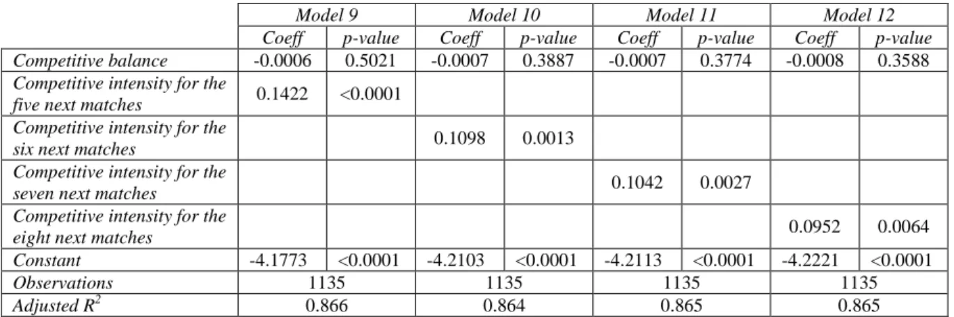
Table 5. Estimates of the attendance equation for competitive balance and competitive intensity for the four last temporal horizons3

Coeff p-value Coeff p-value Coeff p-value Coeff p-value Competitive balance -0.0006 0.5021 -0.0007 0.3887 -0.0007 0.3774 -0.0008 0.3588 Competitive intensity for the

five next matches 0.1422 <0.0001 Competitive intensity for the

six next matches 0.1098 0.0013

seven next matches 0.1042 0.0027

eight next matches 0.0952 0.0064

Constant -4.1773 <0.0001 -4.2103 <0.0001 -4.2113 <0.0001 -4.2221 <0.0001

Observations 1135 1135 1135 1135

Adjusted R2 0.866 0.864 0.865 0.865

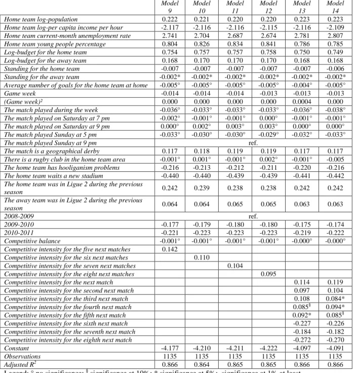
We tested two other models in incorporating the eight temporal horizons for which only a possibility of reversal during the larger number of matches and not before is taken into account. The results are reported in Table 6 with Model 13 for only sure ranks and Model 14 for sure and potential ranks.

Table 6. Estimates of the attendance equation for competitive balance and competitive intensity with the eight temporal horizons for which only a possibility of reversal during the larger number of matches and not before is taken into account4

Model 13 Model 14

Coeff p-value Coeff p-value

Competitive balance -0.0003 0.6770 -0.0003 0.6821

Competitive intensity for the next match 0.1135 0.0016 0.1192 0.0001 Competitive intensity for the second next

match 0.0970 0.0099 0.1037 0.0060

Competitive intensity for the third next

match 0.1077 0.0073 0.0839 0.0447

Competitive intensity for the fourth next

match 0.0847 0.0713 0.0942 0.0481

Competitive intensity for the fifth next

match 0.0922 0.0451 0.0849 0.0732

Competitive intensity for the sixth next

match -0.2273 0.0007 -0.2260 0.0007

Competitive intensity for the seventh

next match -0.1838 <0.0001 -0.1824 <0.0001

Competitive intensity for the eighth next

match -0.2719 <0.0001 -0.2700 <0.0001

Constant -4.0973 <0.0001 -4.0906 <0.0001

Observations 1135 1135

Adjusted R2 0.866 0.866

With only sure ranks, the horizons of one, two and three matches have a significantly positive impact at the 1% level, the horizon of four matches a significantly positive impact at the 10% level, the horizon of five matches a significantly positive impact at the 5% level and the horizons of six, seven and eight matches a significantly negative impact at the 1% level. The fact that the horizon of four matches is less significant than the one of five matches can seem surprising. With sure and potential ranks, the horizons of one and two matches have a significantly positive impact at the 1% level, the horizons of three and four matches a

3

Full estimates are available in Appendix.

4

(12)

significantly positive impact at the 5% level, the horizon of five matches a significantly positive impact at the 10% level and the horizons of six, seven and eight matches a significantly negative impact at the 1% level. These results are more consistent than the ones with only sure ranks. They could indicate that spectators are interested in both sure and potential ranks and not only in sure ranks. We envisage the implications of such a result in the following section.

6. Discussion, implications and avenues 6.1. Discussion

It is important to know on which match temporal horizon spectators consider there is uncertainty of outcome. Indeed, it gives indications about the optimal format of the contest. If the match temporal horizon is large, sporting stakes can be limited but if the match temporal horizon is small, it is necessary to have sufficient sporting stakes so as to optimize the number of teams in contention.

When we deal with temporal horizons until a given number of matches and not only in a given number of matches (that is to say until the three next matches and not only in three matches for example), the horizon of the three next matches could seem better than one or two next matches since it is the only one among these three horizons which is significantly at the 1% level both for only sure ranks and sure and potential ranks. However, we mention at the end of the previous section that results with sure and potential ranks are more consistent than with only sure ranks. With sure and potential ranks, the temporal horizon of the two next matches is significant at the 1% level as the one for the three next matches. Moreover, when we deal with temporal horizons only in (and not until) a given number of matches with sure and potential ranks, the temporal horizons of one and two matches have a significantly positive impact at the 1% level whereas the temporal horizon of three matches has a significantly positive impact only at the 5% level. Consequently, spectators are more sensitive to uncertainty of outcome when a change on ranks with sporting stakes can happen during the two next matches rather than in three matches. We can conclude that the two next matches are the good temporal horizon to consider there is uncertainty of outcome.

6.2. Implications

The risk of having teams not in contention is obviously stronger with the temporal horizon of the two next matches than with the horizons of the three next matches and above. In European football major leagues which are historically organized without playoffs, that risk confirms the necessity for the teams of a league to be balanced or more precisely that among the different groups of teams (in contention for champion title, qualification in Champions League, in Europa League, to avoid relegation), there are competitive balance and sporting stakes (Scelles, Desbordes and Durand, 2011). Two matches are a good horizon to consider, where the uncertainty of outcome is interesting because it allows the measurement of uncertainty during a championship on the basis of the team’s percentage for which a situation change can arise during the two next game weeks. Scelles et al. (2011) chose such a horizon of two matches to measure intra-championship outcome uncertainty.

Besides, we find that the significance for uncertainty measured through a horizon of one or two matches is better with sure and potential ranks than with only sure ranks. Scelles et al. (2013) obtained no significance difference between only sure ranks and sure and potential ranks with competitive intensity measured by the points difference for the home team with the closer competitor with a different situation. Nevertheless, our results indicate that spectators

(13)

are interested in both sure and potential ranks and not only in sure ranks. Scelles et al. (2011) took into account potential ranks to measure intra-championship outcome uncertainty. The fact that sporting stakes on potential ranks seem to attract spectators gives an argument to keep “La Coupe de la Ligue” for which some French football stakeholders (players, coaches, presidents and even spectators in spite of the previous result!) are not convinced that it is useful because it can delete a qualifying rank in the Europa League.

6.3. Avenues

In another contribution about determinants of attendance in Ligue 1, Scelles et al. (2013) showed that competitive intensity is of prime importance in comparison with competitive balance measured by points difference between the two teams before the match. In this article, we conclude that the two next matches are the good temporal horizon to consider there is uncertainty of outcome and it is necessary to take into account potential ranks (and not only sure ranks) to find consistent results. To pursue these two studies, an interesting work would be to observe if there is a hierarchy among sporting stakes. We expect this is the case and stakes related to champion title and qualification in Champions League are more attractive than those for qualification in Europa League which are more attractive than those to avoid relegation which are more attractive than no sporting stakes. It would be necessary to check this expectation.

In this article, empirical results suggest that Ligue 1 spectators are more sensitive to uncertainty of outcome until a temporal horizon of two matches. But would this finding be the same if the dependent variable is a television audience rating? This question is of prime importance since television rights are the first financial resources for clubs in Ligue 1. An explanation of television audience rating has received little attention in the literature due to the lack of available data. Forrest, Simmons and Buraimo (2005) found a significant positive relationship between outcome uncertainty and the size of television audiences in English Premier League football between 1993 and 2003. Buraimo (2008) estimates a joint attendance-television audience model for the second tier of English football (the Championship) and finds no significant impact of match outcome uncertainty on either gate attendance or television audience. Buraimo and Simmons (2009) find that television viewers prefer close contests to more predictable contests in Spanish football. Nevertheless, none of these studies incorporates our uncertainty of outcome measure. It would be interesting to follow up our work by observing the impact of our outcome uncertainty measure on television audiences. In particular, attention could be focused on match temporal horizon for which it is most relevant to consider whether there is an uncertainty of outcome. It is not certain that television viewers have the same sensitivity as spectators in relation to uncertainty of outcome.

7. Conclusion

In this article, we have estimated an attendance equation for the French football Ligue 1 using data from individual games played during the 2008-2011 period. We included all types of variables (socioeconomic, sectorial and incentives) proposed in the literature as explanatory factors and focused our attention on the impact of competitive intensity measured through dummies that are function of the points difference for the home team before a match in relation to ranks with sporting stakes. Empirical results show that the two next matches is a better horizon than the three next matches and above to consider whether there is uncertainty of outcome from the spectator point of view. This is the case only when we take into account

(14)

potential ranks for qualification in Europa League with which results are more consistent than those with only sure ranks.

In the future, it would be relevant to observe if there is a hierarchy among sporting stakes. A study about television audience ratings would be another interesting extension to the present article. Television rights are now the main financial resources for clubs in Ligue 1. In spite of a new interest in Ligue 1 by Qatari television channel Al Jazeera, it is uncertain whether television channels will continue to finance Ligue 1 at the same level in the future. From this perspective, results about the determinants of television audience ratings could help LFP and television channels to optimize the format of the contest and its income.

References

Andreff, W. (2009) “Équilibre compétitif et contrainte budgétaire dans une ligue de sport professionnel” Revue Economique 60, 591-633.

Buraimo, B. (2005) “Satellite broadcasting and stadium attendance revisited: evidence from the English premier league” Lancashire Business School, University of Central Lancashire, Preston PR1 2HE, UK.

Buraimo, B. and Simmons, R. (2009) “A tale of two audiences: spectators, television viewers and outcome uncertainty in Spanish football” Journal of Economics and Business 61, 326-338.

Forrest, D., Simmons, R. and Buraimo, B. (2005) “Outcome uncertainty and the couch potato audience” Scottish Journal of Political Economy 52, 641-661.

Fort, R. and Maxcy, J. (2003) “Comment: Competitive balance in sports leagues: An introduction” Journal of Sports Economics 4, 154-160.

Gayant, J.P. and Le Pape, N. (2012) “How to account for changes in the size of Sports Leagues? The Iso Competitive Balance Curve” Economics Bulletin 32, 1715-1723.

Groot, L. (2008) Economics, uncertainty and European football: Trends in competitive

balance, Edward Elgar: Cheltenham, UK / Northampton, MA.

Humphreys, B.R. (2002) “Alternatives measures of competitive balance in sports leagues”

Journal of Sports Economics 3, 133-148.

Kesenne, S. (2000) “Revenue sharing and competitive balance in professional team sports”

Journal of Sports Economics 1, 56-65.

Kringstad, M. and Gerrard, B. (2004) “The concepts of competitive balance and uncertainty of outcome” International Association of Sports Economists Conference Paper 0412.

Kringstad, M. and Gerrard, B. (2005) “Theory and evidence on competitive intensity in European soccer” International Association of Sports Economists Conference Paper 0508. Kringstad, M. and Gerrard, B. (2007) “Competitive balance in a modern league structure” Communication abstract to the North American Society for Sport Management Conference, May 30 – June 2, Ft. Lauderdale, Florida, 26-27.

(15)

Lee, T. (2010) “Competitive balance in the national football league after the 1993 collective bargaining agreement” Journal of Sports Economics 11, 77-88.

Scelles, N., Desbordes, M. and Durand, C. (2011) “Marketing in sport leagues: optimising the product design. Intra-championship competitive intensity in French football Ligue 1 and basketball Pro A” International Journal of Sport Management and Marketing 9, 13-28.

Scelles, N., Durand, C., Bonnal, L., Goyeau, D. and Andreff, W (2013) “Competitive balance versus competitive intensity before a match: is one of these two concepts more relevant in explaining attendance? The case of the French football Ligue 1 over the period 2008-2011”

Applied Economics 45, 4184-4192.

Szymanski, S. (2001) “Income inequality, competitive balance and the attractiveness of team sports: some evidence and a natural experiment from English soccer” The Economic Journal 111, F69-F84.

Szymanski, S. (2003) “The economic design of sporting contests” Journal of Economic

Literature 41, 1137-1187.

White, H. (1980) “A heteroskedasticity-consistent covariance matrix estimator and a direct test for heteroskedasticity” Econometrica 48, 817-838.

Zimbalist, A.S. (2002) “Competitive balance in sports leagues: an introduction” Journal of

(16)

Appendix

Table A1: Full estimates of the attendance equation for Models 9 to 14

Model 9 Model 10 Model 11 Model 12 Model 13 Model 14

Home team log-population 0.222 0.221 0.220 0.220 0.223 0.223

Home team log-per capita income per hour -2.117 -2.116 -2.116 -2.115 -2.116 -2.109 Home team current-month unemployment rate 2.741 2.704 2.687 2.674 2.781 2.807 Home team young people percentage 0.804 0.826 0.834 0.841 0.786 0.785

Log-budget for the home team 0.754 0.757 0.757 0.758 0.750 0.749

Log-budget for the away team 0.168 0.170 0.170 0.170 0.168 0.168

Standing for the home team -0.007 -0.007 -0.007 -0.007 -0.007 -0.006 Standing for the away team -0.002* -0.002* -0.002* -0.002* -0.002* -0.002* Average number of goals for the home team at home -0.005° -0.005° -0.005° -0.005° -0.004° -0.005°

Game week -0.014 -0.014 -0.014 -0.013 -0.013 -0.013

(Game week)² 0.000 0.000 0.000 0.000 0.0004 0.000

The match played during the week -0.036° -0.033° -0.033° -0.033° -0.036° -0.038° The match played on Saturday at 7 pm -0.002° -0.001° -0.001° 0.000° -0.001° -0.001° The match played on Saturday at 9 pm 0.000° 0.002° 0.003° 0.003° 0.000° 0.000° The match played Sunday at 5 pm -0.033° -0.030° -0.030° -0.029° -0.032° -0.033°

The match played Sunday at 9 pm ref.

The match is a geographical derby 0.117 0.118 0.119 0.119 0.117 0.117 There is a rugby club in the home team area -0.001° 0.001° -0.001° 0.002° -0.001° -0.005 The home team has hooliganism problems -0.216 -0.213 -0.212 -0.211 -0.220 -0.216 The home team waits a new stadium -0.440 -0.440 -0.439 -0.439 -0.441 -0.442 The home team was in Ligue 2 during the previous

season 0.242 0.239 0.238 0.238 0.242 0.242

The away team was in Ligue 2 during the previous

season 0.064 0.064 0.065 0.065 0.063 0.063

2008-2009 ref.

2009-2010 -0.177 -0.179 -0.180 -0.180 -0.175 -0.174

2010-2011 -0.221 -0.223 -0.223 -0.223 -0.219 -0.222

Competitive balance -0.001° -0.001° -0.001° -0.001° -0.000° -0.000° Competitive intensity for the five next matches 0.142

Competitive intensity for the six next matches 0.110

Competitive intensity for the seven next matches 0.104

Competitive intensity for the eight next matches 0.095

Competitive intensity for the next match 0.114 0.119

Competitive intensity for the second next match 0.097 0.104