HAL Id: inria-00390312
https://hal.inria.fr/inria-00390312
Submitted on 1 Jun 2009
HAL is a multi-disciplinary open access
archive for the deposit and dissemination of
sci-entific research documents, whether they are
pub-lished or not. The documents may come from
teaching and research institutions in France or
abroad, or from public or private research centers.
L’archive ouverte pluridisciplinaire HAL, est
destinée au dépôt et à la diffusion de documents
scientifiques de niveau recherche, publiés ou non,
émanant des établissements d’enseignement et de
recherche français ou étrangers, des laboratoires
publics ou privés.
Adaptive torsion-angle quasi-statics: a general
simulation method with applications to protein
structure analysis and design.
Romain Rossi, Mathieu Isorce, Sandy Morin, Julien Flocard, Karthik
Arumugam, Serge Crouzy, Michel Vivaudou, Stephane Redon
To cite this version:
Romain Rossi, Mathieu Isorce, Sandy Morin, Julien Flocard, Karthik Arumugam, et al..
Adap-tive torsion-angle quasi-statics: a general simulation method with applications to protein structure
analysis and design.. Bioinformatics, Oxford University Press (OUP), 2007, 23 (13), pp.i408-17.
�10.1093/bioinformatics/btm191�. �inria-00390312�
Adaptive Torsion-Angle Quasi-Statics: a General
Simulation Method with Applications to Protein Structure
Analysis and Design
Romain Rossi
1, Mathieu Isorce
2, Sandy Morin
1, Julien Flocard
2, Karthik
Arumugam
2, Serge Crouzy
2, Michel Vivaudou
3, Stephane Redon
1 ∗1i3D GRAVIR - INRIA Rhone-Alpes, 655 avenue de l’Europe, 38334 Saint Ismier Cedex, France, 2Laboratoire de Chimie et Biologie des M ´etaux, Institut de Recherches en Technologies et
Sciences pour le Vivant, Universit ´e Joseph Fourier UMR 5249, CEA Grenoble, 17, rue des martyrs, 38054 Grenoble Cedex 9, France3Institut de Biologie Structurale, UMR5075 CEA-CNRS-Univ. J.
Fourier 41, rue Jules Horowitz, 38027 Grenoble, France
ABSTRACT
Motivation: The cost of molecular quasi-statics or dynamics
simu-lations increases with the size of the simulated systems, which is a problem when studying biological phenomena that involve large mole-cules over long time scales. To address this problem, one has often to either increase the processing power (which might be expensive), or make arbitrary simplifications to the system (which might bias the study).
Results: We introduce adaptive torsion-angle quasi-statics, a
gene-ral simulation method able to rigorously and automatically predict the most mobile regions in a simulated system, under user-defined pre-cision or time constraints. By predicting and simulating only these most important regions, the adaptive method provides the user with complete control on the balance between precision and com-putational cost, without requiring him or her to perform a priori, arbitrary simplifications. We build on our previous research on adap-tive articulated-body simulation and show how, by taking advantage of the partial rigidification of a molecule, we are able to propose novel data structures and algorithms for adaptive update of molecu-lar forces and energies. This results in a globally adaptive molecumolecu-lar quasi-statics simulation method. We demonstrate our approach on several examples and show how adaptive quasi-statics allows a user to interactively design, modify and study potentially complex protein structures.
Contact: [email protected] 1 INTRODUCTION
Faced with the significant complexity of the structures and inter-actions that they want to simulate, computational biologists may typically resort to two possible strategies: they can either incre-ase the processing power (e.g. use costly parallel supercomputers), or use simplified representations of the geometry or of the dyna-mics of the involved molecules. Frequently, these simplification methods involve representations in reduced coordinates (e.g. mode-ling the molecule as an articulated body), where subsets of atoms
∗to whom correspondence should be addressed — [email protected]
are replaced by idealized structures (Head-Gordon and Brooks, 1991; Herzyk and Hubbard, 1993), or performing normal-mode or principal components analysis in order to determine the essen-tial dynamics of the system. Because they contain fewer degrees of freedom, these simplified representations allow the biologists to accelerate the computation of the molecular dynamics, and faci-litate the study of the molecular interactions by focusing on the regions of interest. They also make it possible to obtain minimal-energy structures that take experimental constraints into account more efficiently.
However, current geometry or dynamics simplification methods have a fundamental flaw: they are unable to automatically determine the level of detail which best describes a given molecular interac-tion. Thus, the biologist must have some prior structural knowledge about the interaction he wishes to model before choosing the best representation; he must choose the simplest representation of the molecules, i.e. the most efficient in terms of computational cost, which still allows precise simulations of the biological phenomenon under study. In other words, there is currently no method that auto-matically determines which parts of the molecule must be precisely simulated, and which parts can be simplified without affecting the study of the molecular interaction. Such an adaptive simplification method would greatly facilitate the study of biological phenomena for which there lacks sufficient structural information, and would help reduce the need for costly supercomputers currently required to simulate complex biological molecules.
In this paper, we introduce adaptive torsion-angle quasi-statics, a general technique to rigorously and automatically determine the most important regions in a simulation of molecules represented as articulated bodies. At each time step, the adaptive algorithm deter-mines the set of joints that should be simulated in order to best approximate the motion that would be obtained if all degrees of free-dom were simulated, based on the current state of the simulation and user-defined precision or time constraints. We build on our previous research on adaptive articulated-body simulation (Redon and Lin, 2006; Redon et al., 2005) and show how, by taking advantage of the partial rigidification of a molecule, we are able to propose novel data structures and algorithms for adaptive update of molecular
Redon et al.
forces and energies. This results in a globally adaptive molecu-lar quasi-statics simulation method. We demonstrate our approach on several examples and show how adaptive quasi-statics allows a user to interactively design, modify and study potentially complex protein structures1.
Organization: The paper is organized as follows. Section 2 descri-bes the prior research on which our algorithm is based. Section 3-6 introduce novel data structures and algorithms for adaptive update of molecular forces and energies. Section 7 describes several results obtained with our method, and Section 8 concludes and lists a few research directions we want to investigate.
2 ADAPTIVE QUASI-STATICS
We begin by providing an overview of our previous work on adap-tive quasi-statics (Redon and Lin, 2006) and dynamics of articulated bodies (Redon et al., 2005). Note that we do not provide the details of the equations, as these are not needed to understand this paper’s contribution, and would unnecessarily lengthen the exposition. The interested reader may refer to the aforementioned papers.
2.1 Forward quasi-statics of articulated bodies
The forward quasi-statics problem refers to the computation of the joint accelerations of an articulated body, based on its current state and the forces applied to it — assuming the joint velocities are zero at all time. In the case of an articulated-body representation of a molecule, this amounts to determine the accelerations of the torsion angles, under a zero temperature assumption (or infinite “friction”). Our adaptive quasi-statics algorithm relies on the divide-and-conquer algorithm(DCA, Featherstone, 1999a,b). In this algorithm, an articulated body is recursively defined by connecting two articu-lated bodies. The sequence of assembly operations is described in a binary assembly tree, in which the leaf nodes represent rigid bodies, and the root node corresponds to the complete articulated body (see Figure 1). Each non-leaf node represents both a sub-articulated body and the joint used to connect its two child nodes.
Similar to the Newton-Euler equations characterizing the dynamics of rigid bodies, Featherstone (1999a,b) shows that the dynamics of an articulated body can be described by the following articulated-body equation:
a = Φf + b, (1) where a is the composite acceleration of the articulated body (a vec-tor which concatenates the bodies accelerations), Φ is the composite inverse inertia of the articulated body, f is a composite kinematic constraint force (which holds the articulated body together), and b is a composite bias acceleration, due to external forces and torques (inertial effects are zero under the quasi-statics assumption). Featherstone’s DCA essentially consists in two passes over the com-plete assembly tree. The main pass is a bottom-up traversal, in which the DCA determines the inverse inertias and bias accelera-tions for each node in the assembly tree from those of its children.
1 Note that a few powerful tools already exist for structure modification
(e.g. Crivelli et al. (2004). To the best of our knowledge, however, these tools rely on arbitrary user-defined simplifications or external quasi-statics or dynamics solvers, which might be too costly when the system increases.
The main pass starts by computing the coefficients of the leaf nodes (the rigid bodies):
Φ = I−1 b = I−1fk, (2)
where I is the 6 × 6 spatial inertia of the rigid body, and fk is an
external (i.e. non-constraint) force applied to the rigid body. Then, assuming C denotes an articulated body formed by assembling two articulated bodies A and B:
ΦC= ΦC(ΦA, ΦB) bC= bC(bA, bB, QC), (3)
where QC is a torque applied to the joint connecting A and B. When the main pass is complete, the top-down back-substitution passrecursively computes the kinematic constraint forces fAand
fB(which enforce the kinematic constraint between A and B) and the acceleration ¨qCof the joint connecting A and B:
(fA, fB) = f (fC) ¨qC= ¨qC(ΦA, ΦB, fC). (4) For the root node, the kinematic constraint forces are zero2.
2.2 Adaptive quasi-statics of articulated bodies
2.2.1 Hybrid bodies. When the external forces are known, the complexity of the DCA is linear in the number of joints in the articulated body, since all nodes of the assembly tree have to be traversed. This is optimal (since the forward quasi-statics problem is to compute all joint accelerations), and cannot be improved on. Thus, in order to speed up the simulation, we approxima-tely solve the forward quasi-statics problem by computing joint accelerations in a limited sub-tree of the assembly tree (cf Figure 1), that we call the active region. The remaining joints are inac-tive (their accelerations being implicitly set to zero). We call an articulated body with at least one inactive joint a hybrid body.
Fig. 1. Assembly tree of an articu-lated body. Adaptive articuarticu-lated-body dynamics simulates only some of the joints in the articulated bodies, which form the active region.
The motion of a hybrid body is simulated by “rigidify-ing” the inactive joints. This results in hybrid inverse iner-tias and bias accelerations Φ and b, that can also be com-puted from the bottom up, according to a hybrid version of Eq. (3) (Redon and Lin, 2006).
Note that, because of the bottom-up dependency in Eq. (3), a force applied to a rigid body has an effect not only on the leaf node
repre-senting the rigid body but also on all its ascendent nodes. Similarly, a torque applied to a joint has repercussions on the node represen-ting the joint and on its ascendent nodes. We thus call force update regionthe set of nodes thus affected by forces and torques. Finally,
2 In the DCA, the articulated-body equations of each assembly node refers
to a limited number of locations in the articulated body, the handles, so that the root node of a floating articulated body (such as a molecule) has no kinematic constraint (cf Featherstone, 1999a,b).
we call update region the union of the active region and the force update region.
A key feature of our adaptive algorithm is the hierarchical kinema-tics representation used to store coefficients (Redon and Lin, 2006). In particular, each node has a principal reference frame, and caches coordinates transformations from its principal reference frame to the principal reference frame of its parent node (the world reference frame, for the root node). Using this hierarchical representation, inverse inertias only depend on joint positions, and are updated in the active region, while bias accelerations depend on joint positions and applied forces and torques, and are maintained in the update region. Overall, hybrid-body quasi-statics are simulated using the following algorithm:
1. Bias accelerations update: We compute the bias accelerations in the update region using hybrid equations.
2. Acceleration update: The accelerations of the active joints are computed.
3. Position update: The positions of the active joints are updated using their accelerations (using e.g. explicit Euler integration). 4. Inverse inertias update: The inverse inertias of the active
nodes are updated, using the new joint positions.
Redon and Lin (2006) show that the complexity of this algorithm is O(na+ nflog(n/nf)), where nais the number of active joints, n
is the total number of joints, and nfis the number of nodes where an
external force of a torque is updated, resulting in potentially signi-ficant performance speed-ups when the number of active joints and external forces updates are low.
2.2.2 Determining the active region. Now that we have a way to reduce the complexity of an articulated body motion, we can address the fundamental problem: how do we determine the joints that should be simulated, in order to best approximate the motion of the articulated body for a given error threshold?
In order to formalize the question, we introduce an acceleration metricin the form of a weighted sum of the joint accelerations in an articulated body3:
A(C) =X¨qTiAi¨qi. (5)
Redon and Lin (2006) shows that the acceleration metric value of an articulated body is a quadratic function of the kinematic constraint forces:
A(C) = (fC)TΨCfC+ (fC)TpC+ ηC, (6) where the acceleration metric coefficients ΨC, pC and ηC can be computed from the bottom up (similar to the articulated-body coefficients). Once the acceleration metric coefficients have been computed (during the main pass), the acceleration metric is used to
3 The rationale behind such a metric is best understood by seeing the
quasi-statics problem as the numerical problem of computing the joint accelerations. Because we are rigidifying some joints (thereby implicitly assuming that their acceleration is zero), the acceleration metric introduced above is a rigorous measure of the error caused by this approximation. Intui-tively, the acceleration metric value of an articulated body is large when one or more of its joints have large accelerations.
restrict the back-substitution pass to the most important sub-tree of the assembly tree. Indeed, the kinematic constraint forces fC can thus serve not only to compute the acceleration of one joint in C (Eq. (4)), but also the acceleration metric value of C, in constant time, before traversing all joint accelerations in C (Eq. 6). Thus, we descend in the assembly tree using a queue which prioritizes nodes based on their acceleration metric value, until a user-defined number of nodes have been processed, or until the remaining error is smaller than a user-defined threshold (Redon and Lin, 2006).
Similar to articulated-body coefficients, the hierarchical state repre-sentation allows for a limited update of the acceleration metric coefficients: in the active region for the position-dependent, quadra-tic coefficients (Ψ), and in the update region for the position- and force-dependent, linear ones (p and η). This allows us to derive the following active region update algorithm, executed periodically:
1. Conversion to the fully articulated state: The hybrid body is converted to its fully articulated state. This step switches back to articulated-body inertias and bias accelerations, and traverses the update region only.
2. Active region determination: We determine the new active region, i.e. the set of joints which are considered to be import-ant at this time step, according to the acceleration metric. This step only traverses the new active region.
3. Conversion to the new hybrid state: The articulated body is converted to the new hybrid state, corresponding to the new active region. Joint accelerations are computed, and the active joint positions are computed accordingly. This step traverses both the former update region and the new active region. Again, this algorithm traverses only a sub-tree of the assembly tree, which may result in significant performance gains. Most import-ant, the acceleration metric ensures that the hybrid motion is a high-quality approximation of the fully articulated motion. In this paper, we present applications of our adaptive framework to proteins. We represent (classically) a protein as an articulated body by simulating all torsion angles: backbone dihedral angles φ and ψ, and side-chain angles ξ. All amino acids are represented as one or more rigid bodies, which may be as small as a single atom, and form the leaves of the assembly tree (see also Section 7).
3 ADAPTIVE PROXIMITY QUERIES
As noted above, the complexity of our adaptive algorithm depends on the number of external forces that have to be updated at each time step. For molecules, forces are typically applied to each atom, and all forces have to be updated at each time step as the con-formation of the molecule evolves. In order to design an adaptive molecular quasi-statics algorithm, we thus need to be able to avoid recomputing all forces at each time step.
Bounding box hierarchy: Typically, distance cutoffs are used to avoid computing negligible forces between distant atoms, and the first stage of the force evaluation step consists in performing pro-ximity queries to detect pairs of interacting atoms, i.e. pairs of atoms that are sufficiently close to each other. Equivalently, in an articulated-body representation of a molecule, the goal is to determine interacting rigid bodies.
Redon et al.
In order to detect interacting rigid bodies, we maintain and use a data structure often used to perform proximity queries bet-ween rigid bodies or articulated bodies: a tree of oriented boun-ding boxes(OBBs, Gottschalk et al., 1996). Precisely, we asso-ciate one OBB to each node in the assembly tree, expressed in the principal reference frame. The OBB of a rigid body is pre-computed and remains constant throughout the simulation. It encloses all atoms composing the rigid body, and is pre-enlarged by a margin corresponding to the user-defined distance cutoff.
Fig. 2. A water cube. The algorithms presented in Sections 3-6 can be rea-dily extended to allow for adaptive update of interactions between groups of molecules (cf Section 7). Dashed lines represent hydrogen bonds.
The OBB of an internal node is computed during the simu-lation, from its two child-ren, in order to enclose them (and, as a result, the atoms within).
Because the OBBs only depend on the positions of the boun-ded atoms, and are expressed in principal reference fra-mes, they are constant in the inactive region. Thus, the bottom-up OBB update step is adaptive as well, and limi-ted to the active region. This adaptive OBB-tree update step is performed at the end of each time step, after the conformation of a molecule has been updated.
Interaction lists: We also maintain interaction lists, i.e. lists of interacting rigid body pairs, for each internal node in the assembly tree. Assume an internal node C is formed by assembling two nodes A and B. Let A1, ..., Aadenote the a rigid bodies in A, and let B1,
..., Bbdenote the b rigid bodies in B. Then, an interaction list of C
references all pairs (Ai, Bj) of interacting rigid bodies — one rigid
body in A, the other in B. Any interaction occurring between two rigid bodies is thus referenced once and only once in the assembly tree, in their deepest common parent.
A key observation is that the interaction state of two rigid bodies in a sub-assembly only depend on their relative positions and orienta-tions, and is thus constant in rigidified sub-assemblies. As a result, interaction lists are constant in the inactive region, and have to be updated in the active region only. In order to keep track of changes in interactions along time, we store two lists per internal node: a list Icof current interactions, and a list Ipof previous interactions.
Adaptive proximity queries: The interactions lists are adaptively updated during the simulation by traversing the OBB hierarchy. Assume a node C is inactive. Then, we know that we do not have to update its interaction list. Moreover, because all descendents of C are inactive as well, their interaction lists do not have to be updated either.
If C is active, however, its interaction list might have changed, so we clear it and rebuild it from scratch using the OBB hierarchy as fol-lows. We first examine whether the OBBs associated to C’s children A and B overlap. If they don’t, we know for sure that the interaction list of C is empty, since the OBBs conservatively enclose the atoms
Algorithm 1 Interaction list update C ← an active node of the assembly tree A ← left child of C
B ← right child of C Q ← queue of node pairs Ic← current interaction list of C
Ip← previous interaction list of C
Ip← Ic
Ic← ∅
Q ← push(A, B) while Q is not empty do
(N1, N2) ← pop(Q)
if OBB(N1) and OBB(N2) overlap then
if N1and N2are rigid bodies then
Ic← push(N1, N2)
else
refine the search by exploring the children of N1and N2
end if end if end while
in A and B, and we can stop the search. If the OBBs associated to A and B overlap, however, we recursively refine the search for interacting rigid bodies by checking for overlaps between the child-ren A.left and A.right of A and the childchild-ren B.left and B.right of B. When the OBBs of two rigid bodies Aiand Bioverlap, the pair
(Ai, Bi) is added to the interaction list of C. In practice, we use a
queue of node pairs to store the OBB pairs that have to be tested for overlap. When the recursion stops, the interaction list of C has been computed.
Algorithm 1 gives a pseudo-code summary of this computation. Note how the previous and current interaction lists are swapped at the beginning of the algorithm, so that current interactions are always stored in Ic. Algorithm 1 is performed in the active region
only. When the molecule has been completely rigidified, the inter-action lists do not have to be updated. Combining effective culling strategies (OBB hierarchies) and adaptive computations allows us to efficiently update the interaction lists of all active nodes, at each time step.
4 ADAPTIVE FORCE UPDATE
We now show that, because all interaction forces (e.g. van der Waals, electrostatic, etc.) only depend on the relative positions and orienta-tions of rigid bodies, we are able to design an adaptive force update algorithm, which takes advantage of the partial rigidification of the molecule to speed up the force computation.
Partial force tables: In order to avoid recomputing all interaction forces at each time step, we associate to each internal node a partial force tablewhich caches some reusable computations. Let C denote an internal node of the assembly tree, and let C1, ..., Csdenote its
s descendent rigid bodies. For any given rigid body Ci, 16 i 6 s,
the partial force fiCis the sum of the spatial forces applied by C1,
..., Ci−1, Ci+1, ..., Cson Ci. Rigid bodies do not have such tables,
since we are not interested in the force applied by rigid bodies onto themselves (they do not deform). The force table associated to the root node of the assembly tree contains, for each rigid body, the total force applied by all other rigid bodies. All partial forces are
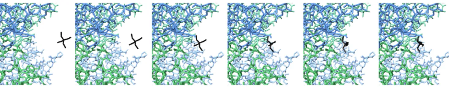
Fig. 3. Interactive structure editing. Quasi-statics simulation allows a user to easily modify structures, by leading the simulated system to the closest local energy minimum. In this example, the user unfolds a poly-alanin with alpha helix structure to form two beta strands. Hydrogen bonds form and help the user build the new structure.
expressed in the principal frame of the rigid body they refer to. This allows the adaptive quasi-static algorithm to avoid recomputing the associated simulation coefficients (cf Section 5). We denote by FC the partial force table of C.
Partial force tables have three important properties. First, they only depend on relative positions and orientations of rigid bodies, and are thus constant for inactive nodes. Like interaction lists and OBB hier-archies, we have to update them in the active region only. Second, the total memory requirement to store all partial force tables is O(n log n), where n is the number of rigid bodies (assuming the assembly tree is balanced). Finally, they can be updated recursively, from the bottom up.
Assume C is formed by assembling A and B, and assume the partial force tables of A and B and the current interaction list of C have been updated. Assume that the a + b rigid bodies in C are indexed as follows: C1 = A1, ..., Ca = Aa, Ca+1= B1, ..., Ca+b= Bb.
The partial force fiCis the sum of the forces applied on Ciby all
other rigid bodies in C.
Assume Cibelongs to A (i.e. Ci= Ai). Then the sum of the forces
applied by rigid bodies in A on Aihas already been computed, and
has been stored in fiA. To compute fiC, we only need to add to fiA
the forces applied by rigid bodies of B interacting with Ai:
fiC= f A i + X Bj,(Ai,Bj)∈ICc fAi←Bj. (7)
The case where Ci belongs to B (i.e. Ci = Ca+j = Bj) is
symmetric: fiC= f B j + X Ai,(Ai,Bj)∈ICc fBj←Ai. (8)
Because of this bottom-up dependency, a change in a partial force stored in a node induces a change in the corresponding partial force stored in the parent node. To easily propagate these changes, each internal node has an update set U , which stores the indices of modified partial forces at the current time step.
Adaptive force update: We can now describe how we use interac-tion lists, partial force tables, and update sets to adaptively update the forces in the simulation, by traversing the active region from the bottom up. The resulting algorithm is directly suggested by equations (7) and (8).
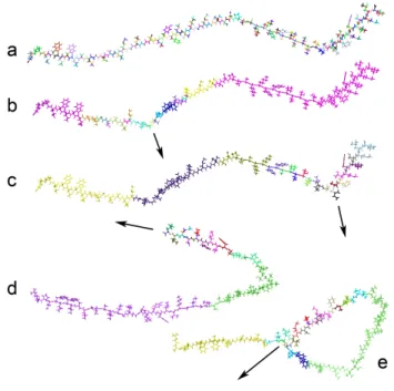
Fig. 4. Adaptive structure modification. The user edits a part of an unfol-ded bacteriorhodopsin (895 atoms and 256 torsion angles). a: the 257 rigid bodies (one color per rigid body). b: the user applies a force (arrow), while allowing only 20 active torsion angles, for better performance. Our adaptive quasi-statics algorithms automatically determine an appropriate, physically-based active region to best approximate the motion that would have been obtained if all degrees of freedom had been active. c: later on, the user app-lies a force at another location, and the algorithm automatically adapts the active region. d: the user pulls an end of the structure. e: when the end pul-led by the user comes close to a previously rigid part, the adaptive algorithm de-rigidifies it to better approximate the resulting interaction.
Let C denote an active internal node formed by assembling A and B. Assume that the partial force tables FA and FB , as well as the previous and current interaction lists IpCand IcC, are known for
the current time step. Our goal is to compute the partial force table FC
for the current time step, based on its values at the previous time step. As noted above, a change in FAor FB, referenced in the
update sets U (A) and U (B), may signal a change in FC. We thus traverse U (A) and U (B) and reset the corresponding entries of FC
to the values stored in FAor FB. For example, if U (A) signals a change in Ai= Ci, we set fiC= f
A i .
Besides changes in FA and FB, three other events — involving interactions between A and B — may cause a change in an entry of FC: (a) an interaction disappears (referenced by IpCbut not by
IcC); (b) an interaction appears (referenced by I C
c but not by I C p);
(c) an interaction is maintained but might be modified (referenced by both IpCand IcC). All three cases may cause a change in an entry
of FC. Therefore, we traverse both IpCand IcCand reset the entries
of FC for each rigid body involved in these interactions. Finally, we complete the update of FCby accounting for current
interacti-ons between rigid bodies of A and rigid bodies of B: we traverse IcC
and, for each interaction (Ai, Bj), we compute the forces fAi←Bj
and fBj←Ai and add them to the corresponding entries in F
C
, fol-lowing equations (7) and (8). Recall that we express fAi←Bj in the
Redon et al.
principal reference of Ai, and fBj←Ai in the principal reference
frame of Bj, similar to all partial forces4.
Algorithm 2 Adaptive force update C ← an active node of the assembly tree A ← left child of C
B ← right child of C
Ic(N ) ← current interaction list of node N
Ip(N ) ← previous interaction list of node N
U (N ) ← update set of node N U (C) ← ∅
for each rigid body R in U (A), U (B), Ip(C) and Ic(C) do
Reset the partial force associated to R in FC Add R to U (C)
end for
for each interaction (Ai, Bj) in Ic(C) do
Compute the interaction forces fAi←Bjand fBj ←Ai fC
i ← fiC+ fAi←Bj
fa+jC ← fC
a+j+ fBj ←Ai
end for
Note that a rigid body Ci not being referenced by any of the lists
U (A), U (B), IC
p and IcCdoes not mean that the partial force fiCis
zero, but only that it hasn’t changed since the previous time step. In summary, we apply algorithm 2 for each node in the active region, from the bottom up. Despite this partial update, we are guaranteed that forces in the simulation are up-to-date.
5 ADAPTIVE COEFFICIENT UPDATE
As noted in Section 2, the adaptive quasi-statics algorithm relies on the ability to cache articulated-body coefficients and acceleration metric coefficients in local reference frames. These coefficients have to be updated only when joint positions or applied forces change. Thanks to the algorithms introduced in Section 3 and 4, we are able to determine on which rigid bodies the applied forces change, and what these changes are. Thus, when algorithm 2 completes, we tra-verse the update set U (C) of the root node C and, for each rigid body Cireferenced in this list, we update the external force applied
to Ciwith the corresponding entry of FC. When all these required
force updates have been performed, we traverse the corresponding force update region(cf Section 2) and update the force-dependent coefficients b, b, p and η. Algorithm 3 summarizes these simple steps.
In summary, at each time step of the simulation, after the confi-guration of the molecule has been updated, we execute the adaptive algorithms 1, 2 and 3 to perform the necessary updates in interaction lists, partial force tables, and simulation coefficients. The simulation can then proceed to the next time step.
6 ADAPTIVE ENERGY UPDATE
In this section, we show how we can also take advantage of the partial rigidification to adaptively update the potential energy of
4 And thus, in general, f
Ai←Bj 6= −fBj←Ai.
Algorithm 3 Adaptive coefficient update C ← the root node of the assembly tree U (C) ← the update set of C for each rigid body Ciin U (C) do
Apply fiCto Ci
end for
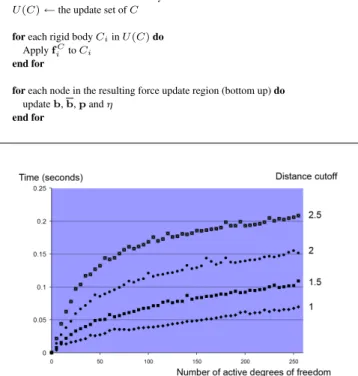
for each node in the resulting force update region (bottom up) do update b, b, p and η
end for
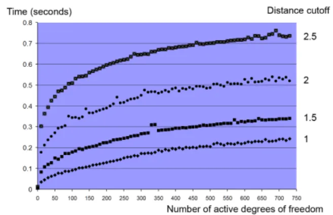
Fig. 5. Performance of the adaptive quasi-statics simulator on the par-tial bacteriorhodopsin model. The cost of one time step is highly correlated with the number of active degrees of freedom and the user-defined distance cutoff (cf Section 7.2.2).
the molecule. Because the algorithm is very similar to the adap-tive force update algorithm, we only briefly describe it. Note that this algorithm can be seen as a generalization of the algorithm intro-duced by Lotan et al. (2004). However, our algorithm only needs n log(n) storage instead of O(n2), which makes it more scalable. Most importantly, our algorithm is able to handle branches in the kinematic structure and can thus model side-chain flexibility (as well as groups of molecules, cf Section 7).
Partial energy tables: Let C be an internal node with c rigid bodies C1, ..., Cc. We call partial energy of Ci, denoted by EiC, the sum
of the potential energies involving Ciand all other rigid bodies in
C: EiC =
Pc
j=1,j6=iEij. Similar to the partial force tables, we
associate to each internal node C a partial energy table EC which
stores the partial energies of the rigid bodies in C. Rigid bodies do not have partial energy tables (equivalently, we set Eii = 0 since
the potential energy of a rigid body is constant). Note how, for any internal node C (including the root node, which describes the com-plete molecule), the sum of the entries in EC is equal to twice the potential energy of C.
Let A and B denote the children of C. As should now be clear after Section 4, the partial energy table EC can be computed from the partial energy tables EA and EB of A and B and the current interaction list IcCof C. Using identical notations, and assuming Ci
belongs to A: ECi = E A i + X Bj,(Ai,Bj)∈IC c E(Ai,Bj). (9) 6
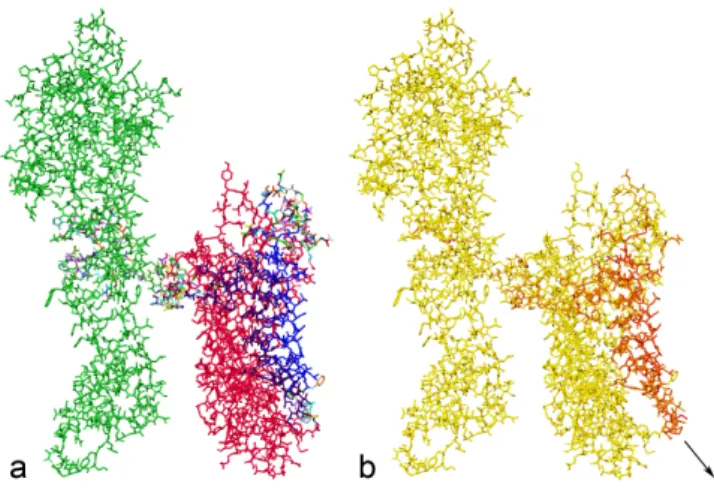
Fig. 6. Modeling signal transduction. a: the initial configuration of RC1. The colors correspond to the rigid bodies (311 rigid bodies containing 6238 atoms). b: the user applies a force to a helix in R0, and visualizes the effect on the linker (center of RC1). A red color indicates regions of high acceleration (cf Section 7.2.3).
If, instead, Cibelongs to B:
EiC= E B j + X Ai,(Ai,Bj)∈IcC E(Ai,Bj). (10)
We can thus update partial energy tables from the bottom-up, and we have to do this in the active region only (since potential energies of rigid bodies are constant). Moreover, we can use the same update sets as in the adaptive force update algorithm, since we use the same interaction lists.
Adaptive energy update: The resulting adaptive energy update algorithm is straightforwardly derived from the adaptive force update algorithm. Essentially, the second for loop is replaced by:
for each interaction (Ai, Bj) in Ic(C) do
Compute the potential energy EAi,Bj EC
i ← ECi + EAi,Bj
ECa+j← EC
a+j+ EAi,Bj
end for
When the configuration of the molecule has been updated at the end of the time step, applying the adaptive energy update algorithm from the bottom up, in the active region only, guarantees that all partial energies in the assembly tree are correct. Summing the partial ener-gies of the root node gives the total potential energy of the molecule.
7 RESULTS
We have implemented our approach in C++ and tested the simula-tor on a 1.7GHz laptop computer with 1GB RAM. In this section, we present a few applications of adaptive molecular quasi-statics to protein structure analysis and design.
7.1 Models
Our framework allows for any (acyclic) branched articulated-body representation of a molecule. Our current implementation handles two classical representations, adapted to torsion-angle simulation:
• the all-atom model, corresponding to the CHARMM22 repre-sentation (MacKerell et al., 1998).
• the extended-atom model, where hydrogen atoms attached to aliphatic carbon atoms are grouped into “extended carbon” atoms, following the CHARMM19 representation (Neria et al., 1996).
These geometric or topological models define the smallest elements in proteins which will be considered as rigid bodies in the simula-tion. They are defined in topology files parsed at the beginning of the simulation. As mentioned above, peptide bonds and cycles are pre-rigidified. We remove from the force fields and energy functi-ons the terms that are cfuncti-onstant in the torsion-angle representation (i.e. the terms relative to bond lengths and angles). Dihedral angles terms are easily expressed as functions of torsion angles.
An extremely useful characteristic of the algorithms presented in Sections 3 to 6 is that they can be extended to groups of mole-cules straightforwardly, by grouping all molemole-cules into a single binary assembly tree. Similar to the definition of an articulated-body in the DCA, we recursively define a molecular assembly as the union of two molecular assemblies. The “leaves” of the mole-cular assembly tree are the assembly trees of the molecules, and the root of the molecular assembly tree describes the complete mole-cular system. Then, instead of applying the algorithms introduced above to each molecule independently, we apply them once, to the molecular assembly tree. This allows us to adaptively update not only the forces and energies that are internal to the molecules, but also the ones which describe the interactions between the molecules, without any modification. Figure 2 shows an example of a simple “water cube” containing 268 water molecules5. The user can inter-act with the molecules and modify the hydrogen bonds network. In the following, we present other examples involving two or more molecules.
7.2 Interactive structure modification
7.2.1 Basic structure editing. The first example is a basic struc-ture edition. Using the quasi-statics simulator, the user turns a poly-alanin with alpha helix structure into a beta hairpin. The simu-lator helps the construction by continuously attempting to optimize the structure. Hydrogen bonds form, and help stabilize the beta hairpin (see Figure 3).
7.2.2 Adaptive structure design. We then demonstrate the adap-tivity of the simulator. The user edits a partial, unfolded model of a bacteriorhodopsin (PDB code 2BRD). The parametrization uses the all-atom model (895 atoms and 256 degrees of freedom). Figure 4 shows how our simulator automatically adapts the active region over time to provide detailed interaction, even though only 20 degrees of freedom are allowed simultaneously. We have measured how the cost of a single time step depends on the number of active degrees of freedom and the user-defined distance cutoff. Figure 5 shows the resulting timings.
7.2.3 Modeling signal transduction. The next example presents an application of adaptive quasi-statics to our current research on
5 The initial configuration of the molecules has been generated using
Redon et al.
Fig. 7. TEA blocking the potassium channel. Even though the initial position of TEA is relatively far away of the entrance of the potassium channel (left), the adaptive quasi-statics algorithm allows to determine the final, equilibrium position in the blocking state without any user intervention (right).
Fig. 8. TEA blocking the potassium channel. The final configuration of TEA, as determined by the adaptive quasi-statics algorithm (cf Section 7.3.1 and Figure 7).
biosensors. Using protein engineering, we are developing novel ultra-sensitive biosensors based on natural receptors fused to natural ion channels acting as electrical probes. In that system, binding of a single ligand to the receptor is transduced into opening or closing of the ion channel. Designing the biosensor requires an understanding of the dynamic interactions between modified membrane proteins to be able to optimize the protein engineering tasks. As the structu-res and mechanisms of membrane proteins are still not well-defined experimentally, interactive molecular modeling can prove useful to study the possible protein-protein interactions in real-time. As an example, we have built a model of a G-protein coupled receptor (R) fused to one monomer of an inwardly-rectifying K+ channel (C). The real biosensor design of R fused to the full tetrameric form of C have been realized and experimental measurements show that a signal is effectively passed from C to R upon binding of a ligand6. Since 3-dimensional structures of R and C were not available in the Protein Data Bank, we have built initial models R0 and C0 by homology with known structures with the program Modeller ( ˇSasli and Blundell, 1993). We have then linked the C-terminal part of R0 and the N-terminal part of C0 with the molecular mechanics pro-gramm CHARMM (Brooks et al., 1983) resulting in a first model for the fused system: RC0. The unstructured region formed by the last ten C-terminal residues of R and the first ten N-terminal resi-dues of C, the linker region, has been experimentally “optimized” by deleting some N-terminal residues of the native form of R to yield the best signal transduction from C to R. We then brought R0 and C0 close to each other and optimized the coordinates of the linker through minimization, using CHARMM. The structure correspon-ding to the minimum energy, called RC1, was retained for our test
6 Details of the assembly of proteins C and R cannot be given at this time
for confidentiality reasons and will be published elsewhere.
in the adaptive simulator. RC1 contains 6238 atoms but, because we were interested in the behavior of the linker region, we pre-rigidified C0 and the helices in R0, which produced an articulated body with 310 degrees of freedom. Figure 6.a shows the initial configuration of RC1, where each rigid body has a different color. Figure 6.b shows how the adaptive simulator was used to study the effect of a force applied by the user to a helix in R0 on the linker. A yellow color indicates regions of low acceleration, while a red color indicates regions with high accelerations. In this example, the motion of the helix is transmitted to the linker.
7.3 Docking
7.3.1 KcsA+TEA. This example demonstrates how quasi-statics simulation can be used to study the docking of small ligands or drugs on to proteins. Tetraethylamonium (TEA) is a classical blocker of potassium channels (e.g. KcsA (Doyle et al., 1998)). From muta-genesis studies, it has been shown that external blockade by TEA is strongly dependent upon the presence of aromatic residue (TYR, PHE, TRP) at a specific position located near the entrance to the pore (Heginbotham and MacKinnon, 1992). The data suggest that TEA interacts simultaneously with the aromatic residues of the four monomers. Our recent molecular dynamics simulations using stan-dard CHARMM force field confirm this idea showing that TEA acts as a real plug inserting in between the 4 TYR residues with its plane perpendicular to the membrane normal (Crouzy et al., 2001). In this experiment, we wanted to check that our algorithm could simulate the docking of TEA into KcsA. We have used our torsion-angle ver-sion of the extended-atom model. All molecules were rigidified, and a distance cutoff of 6 ˚A was used. We positioned the TEA mole-cule outside the channel, in an asymmetric position (see Figure 7-left), and launched the simulation. The quasi-statics algorithm was able to simulate the docking and obtain the final, perpendicular configuration (see Figures 7 and 8).
7.3.2 HPr+P-Ser-HPr. In this second example, we have applied the adaptive quasi-statics simulator to the HPr+P-Ser-HPr com-plex (Janin, 2005). We have selected one couple HPr / P-Ser-HPr in the Protein Data Bank (code 1KKM) and prepared the system using CHARMM. HPr was placed at the origin of the coordinate system and P-Ser-HPr was slightly translated. We then measured the time taken by the adaptive simulator to compute the motion of the mole-cules, per time step, depending on the number of active degrees of freedom and the distance cutoff. Figure 9 reports the resulting trends. As expected, the computational cost is clearly related to the number of degrees of freedom. Moreover, we observe that, for mole-cules in their native state, using larger distance cutoffs tends to result in much larger numbers of interacting atoms, soon producing costly
Fig. 9. Performance of the adaptive quasi-statics simulator in the HPr+P-Ser-HPr study. The cost of one time step is highly correlated with the number of active degrees of freedom and the user-defined distance cutoff (cf Section 7.3.2).
time steps when the number of active degrees of freedom increases. Fortunately, these active degrees of freedom are rigorously selected using the acceleration metric (cf Section 2), enabling the user to obtain meaningful information at interactive rates.
8 CONCLUSION
This paper has introduced the first algorithm for adaptive molecu-lar quasi-statics simulation, which provides the user with complete control on the balance between precision and computational cost, withoutrequiring the need for a priori, arbitrary simplifications. We now want to generalize our work in several directions. From an application point of view, our current implementation only handles proteins, but can be readily extended to other types of molecules. Extension to nucleotides which are also parameterized in classical molecular mechanics force fields will be straightforward. Sugars may be added too, provided that the approximation of rigid rings is valid. Following the strategy used in the water box example, lipid membranes could also be modeled as assemblies of rigid or quasi-rigid phospholipid molecules. Reduced representations could also be adapted (Head-Gordon and Brooks, 1991). When the possibility of introducing symmetries is implemented, viruses may also be inte-resting and challenging systems to study using adaptive simulation. Of course, it would be interesting to study applications of this work to non-biological systems.
From an algorithmic point of view, we want to extend this work to the dynamics case. This will raise the question of physical and biological validation: for example, we will want to compare our approach to classical, non adaptive molecular dynamics simulation. Also, we have noted that, even when few degrees of freedom are active, updating forces and energies might be costly when prote-ins are close to their native states, especially when large distance cutoffs are used. To address this problem, we will investigate exten-sions of classical methods to our adaptive case (e.g. fast multipole). Finally, we note that, similar to Lotan et al. (2004), our adaptive algorithm might be helpful in speeding up Monte Carlo simulati-ons of proteins. Especially, because our method is able to compute an approximation of the gradient of the energy function (equiva-lently, the acceleration of the system), we might be able to design an adaptive hybrid Monte Carlo/ molecular quasi-statics method. Other
topics of interest include various solvent representations, low-level optimizations, use of graphics hardware, parallelization, etc. We strongly believe that our framework could be of great help to biologists who want to easily design, modify and analyze potenti-ally complex protein structures. Our results suggest that adaptive simulation, with its ability to automatically and rigorously focus the processing resources on the most mobile regions of the molecular system, while providing chemically and physically sound configura-tions, may be an important step towards general-purpose, interactive computer-aided molecular analysis and design.
ACKNOWLEDGEMENT
This research was funded by the AMUSIBIO contract (project MDMS NV 2) with the French National Agency of Research in the “Masse de donn´ees” program.
REFERENCES
Brooks, B., Bruccoleri, R., Olafson, B., States, D., Swaminathan, S., and Karplus, M. (1983). Charmm: a program for macromolecular energy, minimization, and dynamics calculations. J. Comput. Chem., 4, 187–217.
Crivelli, S., Kreylos, O., Hamann, B., Max, N., and Bethel, W. (2004). Proteinshop: A tool for interactive protein manipulation and steering. Journal of Computer-Aided Molecular Design.
Crouzy, S., Bern`eche, S., and Roux, B. (2001). Extracellular blockade of k+channels
by tea: results from molecular dynamics simulations of the kcsa channel. J. Gen. Physiol., 118, 207–217.
Doyle, D., Cabral, J., Pfuetzner, R., Kuo, A., Gulbis, J., Cohen, S., Chait, B., and MacKinnon, R. (1998). The structure of the potassium channel: molecular basis of K+conduction and selectivity. Science, 280, 69–77.
Featherstone, R. (1999a). A divide-and-conquer articulated body algorithm for parallel o(log(n)) calculation of rigid body dynamics. part 1: Basic algorithm. International Journal of Robotics Research 18(9):867-875.
Featherstone, R. (1999b). A divide-and-conquer articulated body algorithm for parallel o(log(n)) calculation of rigid body dynamics. part 2: Trees, loops, and accuracy. International Journal of Robotics Research 18(9):876-892.
Gottschalk, S., Lin, M. C., and Manocha, D. (1996). Obbtree: a hierarchical structure for rapid interference detection. In ACM Transactions on Graphics (SIGGRAPH 1996).
Head-Gordon, T. and Brooks, C. (1991). Virtual rigid body dynamics. Biopolymers, 31(1), 77–100.
Heginbotham, L. and MacKinnon, R. (1992). The aromatic binding site for tetrae-thylammonium ion on potassium channels. Neuron, 8, 483–491.
Herzyk, P. and Hubbard, R. E. (1993). A reduced representation of proteins for use in restraint satisfaction calculations. Proteins, 17(3):310-324.
Janin, J. (2005). Assessing predictions of protein-protein interaction: the CAPRI experiment. Protein Sci., 14(2), 278–283.
Lotan, I., Schwarzer, F., Halperin, D., and Latombe, J. (2004). Algorithm and data structures for efficient energy maintenance during monte carlo simulation of proteins. J. Computational Biology, 11(5), 902–932.
MacKerell, A., Bashford, D., Bellott, M., Dunbrack, R., Evanseck, J., Field, M., Fischer, S., Gao, J., Guo, H., Ha, S., Joseph-McCarthy, D., Kuchnir, L., Kuc-zera, K., Lau, F., Mattos, C., Michnick, S., Ngo, T., Nguyen, D., Prodhom, B., III, W. R., Roux, B., Schlenkrich, M., Smith, J., Stote, R., Straub, J., Watanabe, M., Wiorkiewicz-Kuczera, J., Yin, D., and Karplus, M. (1998). All-atom empirical potential for molecular modeling and dynamics studies of proteins. J. Phys. Chem., B 102, 3586–3616.
Neria, E., Fischer, S., and Karplus, M. (1996). Simulation of activation free energies in molecular systems. J. Chem. Phys., 105, 19021921.
Redon, S. and Lin, M. C. (2006). An efficient, error-bounded approximation algorithm for simulating quasi-statics of complex linkages. In Computer-Aided Design, 38, pp. 300-314, Elsevier.
Redon, S., Gallopo, N., and Lin, M. C. (2005). Adaptive dynamics of articulated bodies. In ACM Transactions on Graphics (SIGGRAPH 2005), 24(3).
ˇSasli, A. and Blundell, T. (1993). Comparative protein modelling by satisfaction of spatial restraints. J. Mol. Biol., 234(3), 779–815.