Decision Analysis for Geothermal Energy
by
Keith A. Yost
B.S., Economics, Massachusetts Institute of Technology (2008)
B.S., Nuclear Engineering, Massachusetts Institute of Technology
(2009)
S.M., Nuclear Engineering, Massachusetts Institute of Technology
(2009)
Submitted to the Engineering Systems Division
in partial fulfillment of the requirements for the degree of
Master of Science in Technology Policy
at the
MASSACHUSETTS INSTITUTE OF TECHNOLOGY
ARCHIVES
MASSACHUSETTS INSTrlfTE OF TECHNOLOGYFEB 01
201
LIBRARIES
February 2012
©
Massachusetts Institute of Technology 2012. All rights reserved.
A u t h o r
...
I
...
. . . * ' ' * '
Engineering ystems Division
january 20th, 2012
Certified by...
Herbert Einstein
Professor of Civil Engineering
Th is Supervisor
Accepted by ...
Professor, Aeronautics and
L
Dava Newman
Astronautics and E gineering Systems,
rector, Technology and Policy Program
Decision Analysis for Geothermal Energy
by
Keith A. Yost
Submitted to the Engineering Systems Division on January 20th, 2012, in partial fulfillment of the
requirements for the degree of Master of Science in Technology Policy
Abstract
One of the key impediments to the development of enhanced geothermal systems is a deficiency in the tools available to project planners and developers. Weak tool sets make it difficult to accurately estimate the cost and schedule requirements of a proposed geothermal plant, and thus make it more difficult for those projects to survive an economic decision-making process.
This project, part of a larger effort led by the Department of Energy, seeks to develop a suite of decision analysis tools capable of accurately gauging the economic costs and benefits of geothermal projects with uncertain outcomes. In particular. this project seeks to adapt a set of existing tools, the Decision Aids for Tunnelling, to the context of well-drilling, and make them suitable for use as a core software set around which additional software models can be added.
We assess the usefulness of the Decision Aids for Tunnelling (DAT) by creating two realistic case studies to serve as proofs of concept. These case studies are then put through sensitity analyses designed to reflect project risks to which geothermal wells are vulnerable. We find that the DAT have sufficient flexibility to model geothermal projects accurately and provide cost and schedule distributions on potential outcomes of geothermal projects, and recommend methods of usage appropriate to well drilling scenarios.
Thesis Supervisor: Herbert Einstein Title: Professor of Civil Engineering
Acknowledgments
Above all. I would like to thank my thesis advisor, Prof. Herbert Einstein., for his patient support and guidance during the course of my research. I would also like to thank my friends and research colleagues, who have let me bounce ideas and equations off of them for the better part of two years. Finally, I would like to thank my family-they might not have provided much direct input into the thesis itself, but without them I could not be the person I am today.
Contents
1 Introduction 17
1.1 Problem Statem ent . . . . 17
1.2 Background on Geology and Geothermal Well Drilling . . . . 19
1.3 Structure of the Report . . . . 20
2 Using the Decision Aid for Tunneling for Well-Drilling Applications 23 2.1 A Brief Summary of the DAT and its Features . . . . 23
2.2 The DAT in Depth... . . . . . . . . . . . 29
2.2.1 Areas and Zones. ... . . . . . . .. 29
2.2.2 Ground Parameters and Ground Classes . . . . 31
2.2.3 The W ell Network . . . . 32
2.2.4 Methods, Geometry. and Method Selection . . . . 34
2.2.5 Activities and Time and Cost Equations. . . . .. 35
2.2.6 General and Method Variables . . . . 38
2.3 Using the DAT in a Well Drilling Context . . . . 40
2.3.1 Areas and Zones . . . . .. 40
2.3.2 Ground Parameter Sets and Ground Classes . . . . 42
2.3.3 The W ell Network . . . . 42
2.3.4 Methods. Geometry. and Method Selection . . . ... . . . . 43
2.3.5 Activities ... . . . . . . . . 44
2.3.6 General and Method Variables . . . . 44
2.3.7 Time and Cost Equations... . . . . . . . . . 46
3 Applying the DAT to Example Geothermal Wells 47
3.1 The Synthetic Case ... ... 47
3.1.1 Introduction... . . . . . . . .. 47
3.1.2 Description of the Synthetic Case.. . . . . . . . 51
3.1.3 Modeling the Synthetic Case with the DAT. . . . .. 53
3.1.4 Results and Discussion . . . . 62
3.2 The Sandia Case . . . . 66
3.2.1 The Sandia Well Specification . . . . 66
3.2.2 Modeling the Sandia Well with the DAT . . . . 69
3.2.3 Results and Discussion.. . . . . . . . 82
3.2.4 Sensitivity Analysis... . . . . . . . . . . . . 82
4 Results 137 5 Discussion 145 5.1 Interoperability of the DAT With Other Programs . . . . 145
5.2 DAT Input Flexibility... . . . . . . . . 147
5.3 The range of DAT modelling capabilities . . . . 148
5.4 Conclusions... . . . . . . .. 149
6 Bibliograhy 151 A Glossary 153 B Tester Report Estimation 209 B.1 MIT EGS Study Cost Breakdown Inputs . . . . 209
B.2 MIT EGS Study Cost Breakdown Example Snapshot. . . . .. 209
B.3 MIT EGS Study Cost Breakdown Results... . . . . . . . . 209
C ThermaSource Reports 217 C.1 Well Drilling Project Itinerary... . . . . . . . 217
List of Figures
2-1 The Ground Class Determination Window of the DAT . . . . 24
2-2 The Method Determination Window of the DAT . . . . 25
2-3 The Area-Zone Hierarchy of the DAT... . . . . . . . . 26
2-4 A Simple Tunnel Network . . . . 27
2-5 A Summary of the DAT Approach to Construction Modeling . . . . . 28
2-6 The Zone Generation Window of the DAT... . . . . . . .. 30
2-7 An Example Network . . . . 33
2-8 An Example of Non-Literal Well Network Arcs . . . . 34
2-9 Single and Multi-Cycle Modeling Approaches... . . . . .. 35
2-10 Activity Time and Cost Equations... . . . . . . . . 36
2-11 An Example Activity Network . . . . 37
2-12 The Uniform Distribution Function... . . . .. 38
2-13 The Triangular Distribution Function... . .. 39
2-14 The Bounded Triangular Distribution Function... . . . . . .. 40
2-15 The Lognormal Distribution Function.. . . . . . . . 41
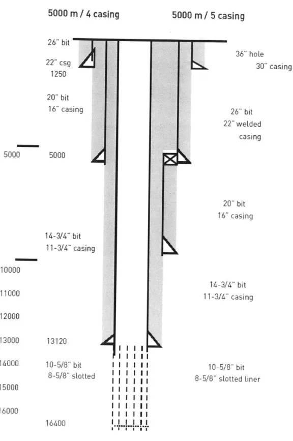
2-16 Activities Do Not Need to Directly Relate to Construction Processes 45 3-1 A Comparison of Two Base-Case Wells... . . . . . 49
3-2 A High-Level Breakdown of Well Project Costs . . . . 50
3-3 The Synthetic Case, the Areas Screen . . . . 54
3-4 The Synthetic Case, the Zones Screen . . . . 54
3-5 The Synthetic Case. the Ground Parameters Screen. . . . .. 55
3-7 The Synthetic Case, the Method Definition Screen . . . . 58
3-8 The Synthetic Case, the Activity Network Screen . . . . 59
3-9 The Synthetic Case, the Activities Screen . . . . 60
3-10 The Synthetic Case, the Method Variables Screen . . . . 61
3-11 The Synthetic Case, the General Variables Screen . . . . 61
3-12 The Synthetic Case, the Fixed Costs Screen . . . . 62
3-13 The Synthetic Case, the Activities Screen . . . . 63
3-14 The Synthetic Case, The Final Time vs. Cost Screen . . . . 64
3-15 The Proposed Well Diagram from Sandia National Laboratories . . 67
3-16 The Activity List of the "Surface Drilling" Construction Stage . . . . 70
3-17 The Sandia Well Network, as Entered into the DAT . . . . 72
3-18 The Method-Geometry Pairing... . . . . . . . .. 73
3-19 The Activity Network of the Surface Drilling Method
/
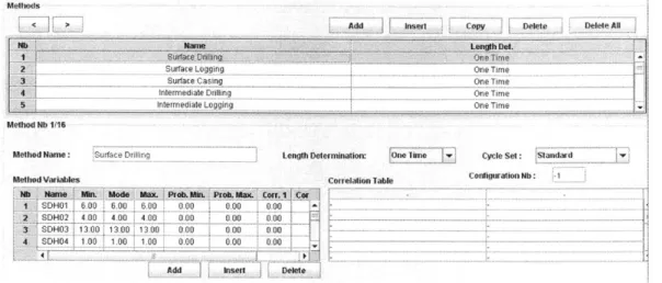
Construction Stage... . . . . . . . . . . . . .. 743-20 DAT Variable Naming Conventions Used in the Sandia Well Example 75 3-21 Time and Cost Equations of the "Surface Drilling" Method . . . . 76
3-22 Example of the Method Variables Depicting Activity Time Requirements 78 3-23 Screenshot From the DAT Providing a List of All General Variables Used in the Sandia Case . . . . 79
3-24 The Sandia Case, the Baseline Result . . . . 84
3-25 Normal Distribution Being Parametrized Into a Triangular Distribution 91 3-26 Lognormal Distribution Being Parametrized Into a Triangular Distri-b u tion . . . . 92
3-27 Screenshot of the DAT's General Variable Window, Employing a Tri-angular, Least-Squared Error Estimation of a Normal Uncertainty . 95 3-28 N=20 Simulations. Normal Uncertainty... . . . . . . . . 96
3-29 N=200 Simulations. Normal Uncertainty... . . . . . . .. 97
3-30 DAT Implementation of Bounded Triangular Distributions . . . . 98
3-31 Example of One Method of Normal Approximation Using a Bounded Triangular Distribution... . . . . . .. 99
3-32 Screenshot of the DAT's General Variable Window, Employing a
Tri-angular, Least-Squared Error Estimation of a Normal Uncertainty . . 100
3-33 N=20 Simulations, Normal Uncertainty (Adjusted).. . . . .. 102
3-34 N=200 Simulations, Normal Uncertainty (Adjusted).. . . . . ... 103
3-35 Screenshot of the DAT's General Variable Window, Employing a Tri-angular, Least-Squared Error Estimation of a Normal Uncertainty . . 107
3-36 N=20 Simulations, Lognormal Uncertainty... . . . . . . . . . 108
3-37 N=200 Simulations, Lognormal Uncertainty.... . . . . . . . 109
3-38 The Activity Network, Including Trouble Activities.. . . . ..111
3-39 Trouble Activity Equations . . . 113
3-40 The Trouble Event Distributions... . . . . . . . . 115
3-41 N=20 Simulations, Trouble Event Sensitivity.. . . . . . . 116
3-42 N=200 Simulations, Trouble Event Sensitivity... . . . . . . . 117
3-43 A Screenshot of the DAT Method Screen. Showing Method Duplication 120 3-44 Screenshot of the DAT's Method Variable Screen, Highlighting the Differences in Method Variable Values Between the Surface Drilling Method Used in Low Strength Geology vs. High Strength Geology . . 121
3-45 Screenshot of the Activity Network for the Intermediate Drilling (High Abrasion, Normal Strength) Stage . . . 123
3-46 Screenshot of the DAT's Method Selection Screen . . . 124
3-47 The Markov Assumptions Used in the DAT Model of Geological Sen-sitivity... . . . . . . . . . 125
3-48 An Illustration of Cycle Length... . . . . . . . . . . . .. 127
3-49 The Activity Equations of the Surface Drilling Stage. Revised for a M odified Cycle Length . . . . 128
3-50 The Results of the Geological Sensitivity Analysis . . . . 129
3-51 Screenshot of the DAT's Method Selection Screen . . . . 132
3-52 Screenshot of the DAT's General Variables Screen for the Holistic Sen-sitivity Analysis... . . . . . . . . 133
4-1 200 Simulated Results From the Synthetic Case . . . . 138
4-2 The Simulated Result from the Deterministic Sandia Case . . . . 139
4-3 200 Simulated Results from the Sandia Case Component Cost Sensi-tivity Analysis (Normal Uncertainty) . . . . 140 4-4 200 Simulated Results from the Sandia Case Component Cost
Sensi-tivity Analysis (Lognormal Uncertainty) . . . . 141 4-5 200 simulated Results from the Sandia Case Trouble Event Sensitivity
Analysis... . . . . . . . . 142
4-6 200 Simulated Results from the Sandia Case Geological Sensitivity
Analysis... . . . . . .. 143
4-7 2000 Simulated Results from the Sandia Case Holistic Sensitivity Analysis 144
5-1 Screenshot of the DAT's XML Save Screen
A-i Abnormal Pressure... A-2 Annular Blowout Preventer
A-3 Bottomhole Assembly . . . .
A-4 An Example Caliper Log . .
A-5 Casing . . . . A-6 Casing collar or Coupling. . A-7 Casing Hanger . . . . A-8 Casing String . . . . A-9 Differential Sticking . . . . . A-10 Directional Drilling... A-I1 Filter Cake . . . .
A-12 Fishing Tool . . . . . ..
A-13 Flange . . . .
A-14 Float Collar . . . .
A-15 Float Shoe . . . .
A-16 Hydraulic Packer. . . ..
A-17 Jar... . . . . . . .. 146 154 155 159 161 163 164 165 167 170 172 174 176 177 178 180 184 187
A-18 Kelly.. . . . . . . . 188
A-19 Overpressure... . . . . . . . . 194
A -20 Packer . . . . 196 A-21 Tool joint. The enlarged, threaded ends of drillpipe ensure strong
connections that withstand high pressures. This diagram shows the enlargement, known as upset, and the threads at the end of the joint. 202
A -22 Topdrive . . . . 203 A-23 W ellhead . . . . 207
List of Tables
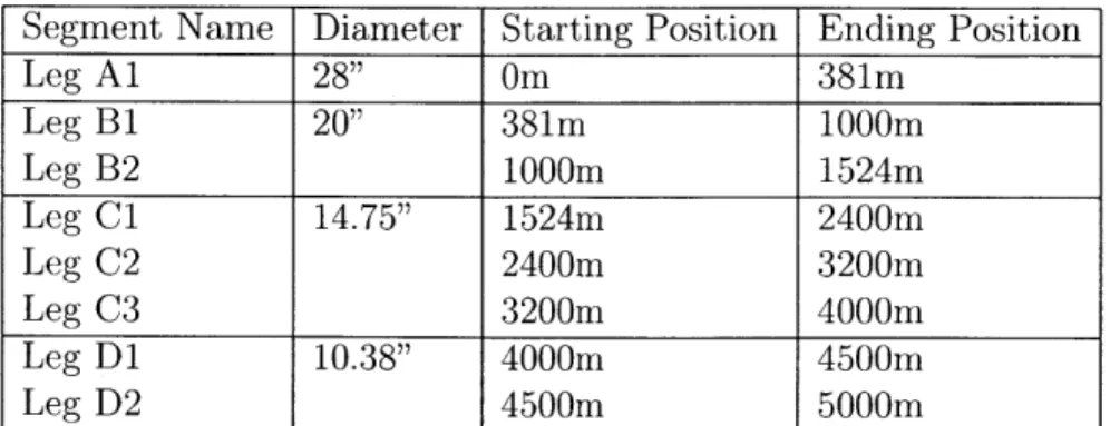
3.1 A Breakdown of the Well Dimensions Used in the Synthetic Example 51
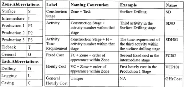
3.2 A List of Abbreviations Used to Designate Types of Well Construction
A ctivity . . . . 68 3.3 A Listing of How Many Activities Constitute Each Construction Stage.,
the Time They Take to Complete in Summary, and a Description of the Typical Constituent Activities... . . . . . . . ... 71
3.4 Individual Contribution of Each Cost Item to the General Hourly Cost 81 3.5 The Assignment of Cost Items Not Assigned to the General Hourly Cost 83
3.6 Mean and Standard Deviation of Geothermal Well Materials Costs. . 87
3.7 Matching of Sandia's Uncertainty Estimates to ThermaSource's Cost Categories... . . . . . . . . 88 3.8 Estimated Cost Uncertainty on the Cost Components used by
Ther-m aSource . . . . 90 3.9 Parameters for the Triangular Distribution on Each DAT Variable
(Normal Scenario)... . . . . . . . . 94
3.10 Parameters for the Triangular Distribution on Each DAT Variable
(Normal Scenario)... . . . . . . . ... 101 3.11 Parameters for the Triangular Distribution on Each DAT Variable
(Lognormal Scenario)... . . . . . . . ... 106 3.12 Parameters for the Triangular Distribution on Each Trouble Activity
Schedule Distribution. . . . . . . . . 114
3.13 Drill Bit Rate of Penetration and Summary Drilling Rate Assumptions
3.14 Drill Bit Rate of Penetration and Summary Drilling Rate Assumptions Made by Sandia and ThermaSource... . . . . ... 122
3.15 The Activity Additions and Subtractions of Each Method . . . . 123
3.16 The Nine Different Geological Conditions Simulated With the DAT . 124
3.17 The Assumed Probability of Encountering a Trouble Event for
Con-structing the Entire Sandia Well in Each of the Ground Classes . . . 130 3.18 The Full Set of Parameters for the Triangular Distribution on Each
Chapter 1
Introduction
1.1
Problem Statement
In developing decision analysis tools for geothermal energy, one of the most important areas of analysis is the cost and time associated with exploration, production, and injection well drilling. Intelligent management of the well drilling process is important for traditional geothermal power, where these activities represent 30% of the total capital cost, but is even more important for enhanced geothermal systems (EGS) where exploration and drilling account for 60% or more of the capital investment [Petty et al, 1992] [Pierce and Livesay, 1993] [Pierce and Livesay, 1994]. Correct and responsive decision making during the well drilling process could prove a critical factor in the economic viability of EGS.
Many efforts at EGS cost and time estimation (e.g. the MIT EGS model and
GETEM) have focused on the problem in aggregate, developing levelized cost
esti-mates that serve the purposes of long-term economic forecasting, but lack the gran-ularity and specificity necessary to aid in projcct management. We focus instead on cost and schedule prediction for the project manager, and aim to develop a tool that (an produce cost and time estimates that are both specific to the particular well being drilled, and detailed enough to aid in making design choices in project planning.
There are multiple sources of uncertainty that make it difficult to estimate the cost and time requirements of geothermal well drilling. These sources of uncertainty
range from traditional project risks, such as input cost fluctuations or failures during construction, to geology related issues, such as poor lithology or lower than expected temperature. As such, a tool that aids the project manager of EGS wells should be flexible enough to accommodate many aspects of design and uncertainty, including well parameters such as depth, production diameter, and drilling angle, site geology parameters such as rock strength, abrasiveness, porosity, and temperature, and po-tential adverse events such as drill string breaks, stuck casing, and detrimental effects due to overpressure or underpressure.
The tools focused on in this report will be based on the Decision Aids for Tunneling
(DAT) also developed at MIT and used in practice. The DAT already have much of
the functionality desired of an EGS cost and time estimation tool, including notably the ability to represent geology and the construction process using a probabilistic approach, as shown in the DAT manual [Min et al, 2009]. While the context may be different (tunnel analysis vs. well analysis), the practical differences between these two applications of the DAT are minimal, and the tools should be capable of producing accurate time-cost distributions with appropriate changes to either the program itself or the way in which the program is utilized by the end user. In addition, the DAT will be integrated with the other decision analysis programs being looked at for this project- for example, some of the geological inputs into the DAT will originate from the GEOFRAC fracture pattern model and supplemented by lithological and other geological information.
In total, there are three potential points of interest to explore. The first is to test how well the DAT can be used to model EGS projects without major modifications. The second is to identify any modifications to the DAT that could enhance their capabilities vis-a-vis geothermal applications. And lastly, the DAT should be eval-uated for compatability with the other elements of EGS decision analysis, including fracturing models. thermal models, surface plant cost and time estimation, etc.
Our goal is to demonstrate the applicability of the Decision Aids for Tunneling to well drilling problems by working through two prototypical examples of injection well drilling. In these examples., the injection well will be modeled as a very simple
sort of tunnel, beginning at the surface, and terminating at the desired well depth. We will demonstrate how the DAT are equipped to model the sources of project risk associated with geothermal well drilling, and thus offer project managers an attractive means of cost and time estimation.
1.2
Background on Geology and Geothermal Well
Drilling
The current state of the art in geothermal drilling is essentially that of oil and gas drilling, incorporating engineering solutions to problems that are specific to the geothermal context, i.e. temperature effects on instrumentation, thermal expansion of casing strings, and lost circulation.
A typical geothermal well drilling project involves three more-or-less distinct
stages of construction: drilling and casing an injection well, hydraulically fractur-ing a volume of rock to prepare a thermal reservoir, and then drillfractur-ing and casfractur-ing one or more production wells into that fractured volume. During plant operation, the injection well will serve as the channel through which a working fluid, typically water, will be pumped underground and passed through the thermal reservoir. After being heated by contact with the hot rock of the reservoir, the working fluid will return to the surface through the production wells.
The order in which these construction activities take place is set by basic con-siderations of the well drilling problem: fracturing must occur after a well is drilled but before it is completely cased, and production wells can only be located once it is known where the fractures have been created.
Radical changes to this construction approach are unlikely. Technological improve-ments to geothermal well drilling are likely to change the speed and cost at which these activities can be performed, but not alter the sequence of activities themselves. Improvements in drilling may result in shorter drill times. better casing may reduce the number of casing strings necessary to secure a wellbore, and improved instruments
may yield more accurate logging of well and geological conditions, but the choices that a project planner faces will stay the same. The constancy of the decision problems associated with EGS well drilling make it an attractive problem for modeling- while the parameters of the problem may change, if the fundamental dynamics do not, then good decision analysis software would avoid obsolescence for some time to come.
Similarly, radical changes to related activities are unlikely as well. Many of the fields adjacent to geothermal well drilling, such as thermal plant technology, are long-established technology- it is unlikely that some other area in EGS will change to a degree that overhauls project planning in well drilling and other subsurface activities. In sum, EGS projects make an ideal arena for decision aids; the projects are complex and require probabilistic estimation, yet are not so dynamic as to thwart computer-aided attempts at decision making.
1.3
Structure of the Report
We divide the remainder of this paper into four distinct sections:
Chapter 2 explains the DAT and their organization. It goes into detail on how cost estimation models are built using the DAT and how this approach would be applied to well-drilling applications. It also briefly discusses modeling techniques that minimize the effort needed to model well-drilling projects.
Chapter 3 describes two proof-of-concept tests for the DAT, one drawn from MIT's report on enhanced geothermal systems, and the other drawn from Sandia research on technological issues in enhanced geothermal systems. These tests consist of of a well design. a modeling of that well design in the DAT. and sensitivity analyses of the well design's cost and completion time. Each of these case studies is advanced as a test of the DAT's functionality; the ease or challenge in modeling these case examples with the DAT is meant to illuminate how the DAT might work as a practical tool of EGS project planning and management. as well as highlight modeling needs left, unmet by the DAT.
presents the outputs that result from DAT modeling work.
Chapter 5 is a discussion of the proof-of-concept tests: what lessons were learned., suggested best-practices for using the DAT in a well-drilling context, potential im-provements to the software, and so on.
In the appendices of this report, we include a glossary of drilling terminology, as well as the relevant sections of the MIT and Sandia reports from which the proof-of-concept tests were drawn.
Chapter 2
Using the Decision Aid for
Tunneling for Well-Drilling
Applications
2.1
A Brief Summary of the DAT and its Features
The Decision Aids to Tunnelling (DAT) approach to modeling revolves around the use of what the DAT term "Methods." A method is comprised of a network of" Activities." The activity network defines the order in which a set of activities takes place. Each activity defines both a cost and a time equation using method-specific variables (called Method Variables) and global variables (called General Variables) whose values are randomly generated by a user-defined probabilistic distribution. To calculate the total cost and schedule of a project., the DAT sum the cost and time results of each method that is utilized by the construction project; the cost and time results are in turn the sum of the cost and time equation results of each activity within the method's activity network. The remainder of this chapter is devoted to explaining the method-based modelling approach in greater detail.
To determine which methods are utilized within a given construction project, the
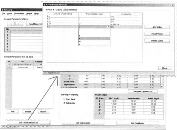
OP S0~ 1- Googr~ O~s Ocflnhwi r1tQd ParameterSets L L M G*round PaitmeoeL Nb 12:r Nb CIP Oveburden Ue1 r 11 .11no4A 10)0 000 030 Start.r, 00500 0 00 0 0 Elga*0*ector 00 0* 0 00 Sitrt0g0robaixiny Nbddnteng*o PUser V" state U Mt het 1000 In Add insert A roudClasses Delete 0.003 Idt erreation Add "whi brS40*l Vah SP -3-30 0000 ~
J
(1(00 000 - 0000 ri (10-3 I 1(000) 000 1d Uoreole 10100 10-00 0100 0 00 .. 0...Figure 2-1: The Ground Class Determination Window of the DAT.
set of geometries and ground classes, and for each possible combination of geometry and ground class, the user specifies a probability that each method will be utilized. Figure 2-1 shows the ground class determination screen of the DAT, while Figure 2-2 shows the method determination screen.
Ground classes are determined through the use of Areas, Zones, and Ground Parameters. An area is a region in which well placement takes place (e.g. from 0 ft to 20000 ft). Zones are subsets of areas, specifying some fraction of the region in which construction takes place, defined either deterministically or probabilistically.
The user defines a set of ground parameters, and each ground parameter has a set of possible states. Within each zone, the user specifies a generation method for each ground parameter. In this manner, the user defines how a set of ground parameters will be probabilistically generated across the entire region in which construction activ-ity takes place. Figure 2-3 provides an example of an Area-Zone-Ground Parameter
Method Definitinn
Grondassa Genmetat Geebuty2 Geemetly3
HJ Undenined Mis(Pn.. lining_1
H Undefined lptem2 ining
it I Undefined alir' ' sng
7 Undefined pattern3 lenma 2
4.V Undefined pattern Sng
L t patter 5 patteir lining 1
1.- pattern pnitem lining_2 4 nattemne eattern 3 lining
L-IV pattern6 pattern d lining_4 L-V Undefined pattern 4 lining 4 Ground Class: R -i Geometry: 2
Deterinistic SetIng pattern 2 Probatublsc Setings Mefiiod pannrn i pattern2_1 pattern 4 pattern 8 crtossnvej ...EPP -&irng_6 Geerneby4 Undefined Undefined Undefined Undefined Undeined Prob Undefined Undefined Undefined Undefined Geomffey5 pattern EPP pallern EPP adtemEPP pattern EPP pattern E PP PattemnEPP pattern EPe pattern EPP _pattemn EPP ga (to 11, tn 0.6
Gtetiy Genweky7 Geomebly' GeomhyI
iarnsover a Undelned lrnng_EPP crnnsoverp rossovery Undefined srung_EFP cressners crossaer v Undefined ling_EPP mrssove_p cronvern Undefined liningEPP rrossverp
inrsoverv a Unnefineg iningEP crosse
-snoverv e nlng_2 Undenned crossnven-p crossover v I nng_2 Undefinen crssover-p cress e:a V Ineng_2 Undefined cissove-p crosover v linng 2 Undefinea tcissoanrep
irssover av In ng 2 Undefined crcssover p
Methori pattern 2 pattern2 22 pattern 3 pattesa EPP ting) emmg_4 ....... Sa a.
0.0
an0 an n-n [JenattprleewetneFigure 2-2: The Method Determination Window of the DAT. Geomeyt Undefined lining5 lIningS5 Undefined Undened linirigd lining 5 llning_6 lining6 Undefined v
Param I Pawrn2 Ground
Class
Area 1 Area 2
Zone 1 Zone 2 Zone 3
Gneiss Schist Granite Gneiss Schist
I-ot
Not Faulted Faulted Faulted Faulted Not Faulted Not Faulted Gneiss/ Gneiss/ Sciist/ Schist/ G uanite/ Grarute/ Gneiss/ Schst/NotFaulted
Not Faulted Faulted Not Faulted Faulted Not Faulted Not Faulted
Faulted
I I I I I
Segment I Sepuent 2 3
Figure 2-3: The Area-Zone hierarchy of the DAT. Within zones, ground parameter values are generated, and these parameter values, in combination with user-supplied logic, define ground classes.
hierarchy.
Ground parameters are used to define ground classes. The user specifies a finite set of ground classes. Then, for each possible combination of ground parameter states, the user assigns a probability to each ground class.
Geometries are determined through a Tunnel Network. A tunnel network (or, in this context, a well network) is a network of construction stages, where each arc in the network specifies a particular geometry, the region in which the arc takes place, and any additional fixed costs or delays. Figure 2-4 is an example well/tunnel network screenshot from the DAT. For each possible combination of geometry and ground class, the user assigns a probability to each method, and then, the DAT define the resulting method used at each locale in the construction region.
The DAT thus use a multi-stage Monte Carlo simulation that generates project costs and schedules as follows: First. the DAT generate the zones within each area.
Then. the DAT generate ground parameter states across the entire region of interest.
Using the resulting sets of ground parameters. the DAT generate ground classes across the entire region of interest. Then. by looking at the geometry specified in each segment of the well network and the ground class(es) that was generated within the region specified in the well segiment. the DAT generate which methods will be used in
e Yew SinutiMn 9i0put iesep
zb~fOmind
Add "Med
ANode Drag Node
MainTunnel Wes latnTunnelEat Dtele Node
AddAt c unnel 4
S 4Drag Arc
Delete AN
Show NOe Name
' Show Node NnRnbet
v Show Arc Namre
J ianApp e Wi-ow
Figure 2-4: A simple tunnel network.
Tunnel
(Tunnel Network + Geometries)Ground Classes
Construction Methods (Excavation Procedures + Supports) Activity Network GC 1 GC 2 CM 2IExcavating Mucking Instling_upport
ow high low high
Advance rate Costlength
Figure 5: A Summary of the DAT Approach to Construction Modeling. Figure
2-5 shows the DAT's layered approach to modeling, taking the construction-specific
conditions (the 'geometry'), and the geological conditions (the 'ground classes') to determine which of a variety of construction methods are used, which in turn define the set of activities that constitute the project, which in turn define the parameters and their probabilistic distributions that will produce the end estimate of cost and time requirements for the project.
the construction process. Figure 2-5, a tunnel example, provides a graphical summary of the DAT approach to modeling.
Once each method has been specified, the DAT begin generating values for the variables that enter into the activity equations within each method. Then, the DAT solve the cost and time equations for each activity, and sum the results from each activity within each used method as well as the fixed delays and costs specified in the well network to output a final cost and time estimation.
G9
2.2
The DAT in Depth
2.2.1
Areas and Zones
The geology along a well can be subdivided into Areas and Zones. An Area is a set of continuous and sequential regions that may consist of only one Zone or many Zones. The term Zone is used to express what can be described as a geologically homogeneous Zone, namely, a stretch of ground in which a particular set of parameters and parameter states may occur. Each of these zones consists of a set of segments, where the term segment refers to a continuous ground section characterized by a specific set of parameter states. As with Areas, Zones may also consist of only one segment. The parameter state sets are usually called Ground Classes. Figure 2-3 is an illustration of the Area-Zone hierarchy.
The Area is the uppermost level of the organization for input in geology. It consists of a set of consecutive Zones.
The Zone is the basic unit of geology for input. It declares a length of ground, and what it consists of.
Zones have three distinct generation methods, labeled within the DAT as Mode 1, Mode 2. and Mode 3. In Mode 1. the zone is estimated to vary between a minimum and maximum length. It generates a variable length between the specificed minimum and maximum values, using the minimum and maximum bounds, and probabilities for minimum. maximum. and modal values. In Mode 2. the zone is estimated to vary between a minimum and maximum endpoint. Similar to Mode 1, it defines the zone using five parameters: a minimum and maximum endpoint, and probabilities for the minimum. maximum. and modal endpoints. Finally. Mode 3 generates a zone length in the same manner as Mode 1. and then checks to make sure that the zone falls between minimum and maximum endpoint values. Figure 2-6 shows a screenshot of
Hed wwo Simu~ation QOtpO Help
S
Read F omRio SavoF~e .Add iser Delet Dele AR
y Name GP Se Gem Mode Mk L MoL L Max.L PreotMin.. 4*tMaX L Mti EP. ocLEA MaxE.P. Pro 11h E.P Ptott Max E
$ sr F SetNC 1 EnOPos, C.0 0 0 I .0 C0 00 600 65000 05000 0 10 003
2 natmbeg Gpset PN 2 End o 000 0 00 0F00 000 800 0500 90 00 0 00
GPeNt EI 03 3 0 00 0 00 > 0 08604 io 0 0
s:2 .F0.tNE 4 L..E.. P 40.00 40 0. 000.. 0.00 0 . .70 0 . . 0-00
5 OF~otN5 EndPos 00 00 00 00 C0 21700 217.0) 21 00 0:00 000
6 s4 'P41Nc. 6 End Pos 00 000 30 000 0 200 2073 500O 0.00 a 00 7 0:5 P *0 End Pos 0.0) 0 0 0.0 0 30400 35407 4 00 700 0 . Zone M 3/23-Zone Nam5 En Pas Mod 2) MEndPos: Mode 57ndpos: U. 10| Max EndPos: . Pro, Ma Endoos;
Figure 2-6: The Zone Generation Window of the DAT. Generation mode 2 (end position) is being used in this example to generate zone sz1. In this particular zone generation, the minimum end position is at 80, the modal end position is at 80, and the maximum end position is at 100.
Ground Paammete Set:
Generadon Mode:
Min Length: Mode Lengh:
Probiain Lengon:
Prob.MUa I ength
2.2.2
Ground Parameters and Ground Classes
Before defining ground classes or distributions of ground parameter states, the user needs to first define the ground parameters. The parameters denote particular geo-logic conditions in a section (usually a zone) of the ground. A parameter usually has several parameter states. An example is the hypothetical parameter Lithology that has the states, Granite, Shale and Gneiss. The user can define the name of parame-ters and their states. GP Name sets the name of the parameter (like Lithology) and
GP state shows the list of possible states for this parameter.
Following this the user will have to define the occurrence of parameters and pa-rameter states, their association with Ground Classes and all other information on the geology. The distribution of parameter states can be determined using five different generation methods: Markov, Fixed Markov, Semi-Fixed Markov, Deterministic, and Semi-Deterministic.
Markov indicates that the parameter states are probabilistically defined using a Markov process. This allows the program to generate certain parameters based on the estimated length and the matrix that defines the probability of transition between all the pairwise sets of ground paramneter states. Specifically, the DAT assign the initial ground state according to the initial probabilities that the user assigns to each state. Then, they determine a length over which the parameter state will remain the same, selecting the length over an exponential distribution of lengths. At the end of this length, there is a probability of transition to each of the other possible parameter states- these probabilities are defined by the user. Upon transition, another length is probabilistically determined from an exponential distribution, and this process continues over the length of the segment over which the ground parameter is generated
using the Markov process.
Fixed Markov produces a Markov-style generation; the difference between it and the "Markov" mode is that, the lengths are first generated based on the mean length and then stay the same (luring the Markov generation. and the Markov generation only takes care of the transition between different states.
Semi-Fixed Markov is an option that allows one to have Markov transitions and triangularly distributed lengths. This is different from "Fixed Markov", which is only based on Markov transitions and fixed length, and from Markov which is based on Markov transitions and exponential lengths.
Deterministic allows the user to deterministically specify the length and state of each segment.
Semi-Deterministic allows the user to specify the state and length of each state probabilistically but in a deterministic sequence. This works very much the same as the definition of the zone sequence.
Ground Classes describe the ground conditions along the well's length and are a particular combination of Parameter States. These Ground Classes will ultimately be used to determine the construction method used to construct a well. Ground Classes are defined by logic rules set by the user- specifically, the user defines a set of ground classes, and for each class defines the set of ground parameters that fall into that class.
2.2.3
The Well Network
Well construction is modeled by first defining the well system followed by the defini-tion of the well geometry (" type cross secdefini-tions"). This informadefini-tion and the geology (Ground Classes), will then be combined to form construction methods.
Specifically, the geology and the well geometry lead to particular excavation pro-cedures and support requirements. The combinations of excavation propro-cedures and support requirements are called Construction Methods.
Since the DAT will eventually produce construction time and cost, the methods need to be described in these terms. The simplest way to do this is in the form of cost per linear unit of well depth drilled and of advance rate. Cost per unit length includes the material-labor-equipment costs to build a unit length of well. Analogously, advance rate expresses the time to build a unit length of well. Rather than express cost and time in this simple way it is possible to simulate construction as a number of parallel or sequential activities (drilling. tripping. circulating. logging.
:1
urface Pump
.Drill
Rig
Surface Drill
2
34
Figure 2-7: An Example Network. Figure 2-7 shows a simple example of a network-in this example, construction begnetwork-ins with the Drill Rig and Surface Pump sections, and as soon as both are complete (the filled circle representing Node 3 indicates an
AND node, while a hollow circle would indicate an OR node), construction of the
Surface Drill section would begin.
casing etc.). In either case other costs such as interest costs, mobilization costs., and cost and time to build other structures can also be considered.
A well network consists of nodes and arcs. Nodes have two functions: they are
endpoints and junctions. In either case. the number of the node has no influence on the simulation, only the type of node will be important. The arcs usually represent physical well sections; each arc is a well section of a single geometry.
The concept of an arc can sometimes be used for types of construction processes different than actual physical well sections. The user may need for example to define more than one well when different construction methods need to be applied in the same well sections at different times. For example, if the lining/casing is placed after the entire well is excavated, the lining process can be represented by defining it as a different construction method in an imaginary "casing arc." Figure 2-8 depicts this example.
Drilling
Arc
Logginc
Arc
Casing Arc
4
Figure 2-8: An Example of Non-Literal Well Network Arcs. Figure 2-8 shows a simple example of a well network, including distinct drilling, logging, and casing stages.
2.2.4
Methods, Geometry, and Method Selection
In addition to specifying well segments by their position, users need to categorize segments by another dimension, called geometry. The geometry category will be used in conjunction with ground class to define the method that will be used over the length of that well segment- it is important therefore to define geometry in a way that aids in proper method selection.
Method selection is a process of user-specified logical rules. much in the same manner as ground class determination. For each pairwise couple of geometry and ground class, the user defines a probability of selection for each of the available methods- most typically. this process will be deterministic, and the user will specify that a geometry-ground class combination will select a particular method in 100% of instances.
Methods themselves are a combination of two features. an activity network, which, through its selection of activities, defines the set of cost and time equations that a method will invoke during a simulation, and a cycle procedure. The latter feature deserves some explanation here- the DAT invoke a method's related cost and time equations once for each "cycle" that occurs within that segment. The method itself defines the length of these cycles- at one extreme, the entire segment could be defined as one cycle, at another. a cycle could be set to be a very small value, thus invoking the method's cost and time equations miultiple times over the construction of that segment. Because the cost and time equations of a method are designed with cycle
Cycle
1
Cycle Length = L, Cycle Number = 1. Cost per Cycle C
Cycle
1 Cycle
2
Cycle
N
Cycle Length = UN, Cycle Number = N, Cost per Cycle = C/N
Construction Stage Length
Figure 2-9: Single and Multi-Cycle Modeling Approaches. If a single cycle is used, then the cost and time equations for that cycle represents the cost and time associated with the entire construction stage. If instead more cycles are used, each cycle incurs only a fraction of the construction stage's total cost and time, with the fraction depending on the number of cycles used.
numbers in mind, there is often no practical difference between breaking an activity into several smaller cycles and invoking small costs with each cycle versus running it over fewer, larger cycles and invoking large costs per cycle. Figure 2-9 illustrates the concept of single vs multi cycle approaches.
Of more importance than cycles are the activity networks and associated activities
that define a method.
2.2.5
Activities and Time and Cost Equations
A Construction Method is described by the so-called Activity Network, and by activity
equations and variables. The construction methods, with their activity networks, activity equations. and numerical variable values, are related to the particular well section. Ground Class. and geometry. The Activity Network contains a sequence of activities represented by arcs. The network relates activities, that is, the sequence in
iFe View Swmioaten t lp JAtpi Ad~t~eM - --- -3 3 -3 excp2 _ 4 eup2 -2 5 eXp23 6 excp3 7 eXcp4 ActMty 12 --0Ud leol~3 t round tength)adv_ ate roud ength0/ady rate round IengthliadYrate6
&W ame eOXtol Nb M-~eU, mode
I atoN rate 34 It L.14 j 0.00
CS -4,t 34 9,24 1.0 C 3.2E_0i340O 3370.221 1G 00
Read 300
GeneralVarlaes
Mb Nzamye. Desd~i n i 14C ax Pr,air. Mn. 0,-oh Ma~
cost*tound_ engtho 1 No 0 cost-toundjengtho 1 No 0 costrounctengthkf 1 No 0 cost1ound length 1 No 0 ... ... ... ... N. 0... Ramurcos
Rb r ble _p Ot. Vae De MhY Mod Max Prob Wn
I s I W Use 1000
-2 lesource 2 r 1l 2000
- - P oodoed 30 00 -
-Resour ce Equatins (Resmacce 1)
Amoun Used V
II
AmoMt Produced - ry2 Tme Equation a undnt
CastEquadon c-st-round -engt..
one Q_ Premptve Calendar Hone
(Java Applt Wrxr
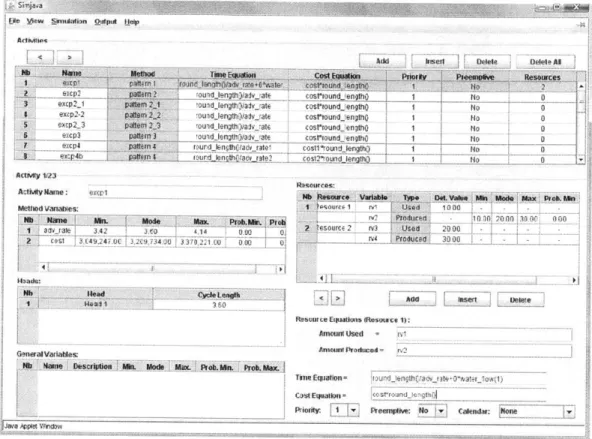
-Figure 2-10: Activity Time and Cost Equations. -Figure 2-10 shows a typical activity screen from the DAT. In this example, each activity has relatively simple time and cost equations, usually involving just two unique parameters: a rate at which the activity proceeds (measured in units of time per unit of length) and a cost per unit length. The example in the figure is a tunnel-based example from the DAT manual.
which they will be performed, to each other. Figure 2-10 shows an example activities screen from the DAT, showing a selection of activities and their associated time and cost equations. Figure 2-11 shows an example activity network.
Each activity defines two equations: a cost equation, which contributes to overall project cost, and a time equation. which contributes to the overall time required to complete the project. These equations can be defined using almost all common operators, as well as any user-defined variables.
Eile View Sinedation O(utpu Hep
Methods
Add Insert Copy Delete Delete Al
Nb Name Lng~hrDet.
Surface Otng (NwrmalAbrasi n Norb malHainesi) O nmw
Surface Logging One Time
n Surface Casing One Time
4 Intermediate Drilling (Normal Abrasion, Normal Hardness) One Time
5Intermedliate Logging one Time
Method Nb 156
H"eHead exe
H ad Nb 1/1--- - - - -- --- Maki up 26" bit and 36"hole osner on r
ActivitNetwork--Make up 26" bit and 36" hole opener on mud motor Pick up 36" stabilizer and cross over to
6-Pickup 36" stabilizer and cross over to 6-5/8" HWDP rNi and open 36" hole with motor and FM
DrII and open 36"hote wit motor and HWDP from 80'to 240'
Circulate C
Trip out of hole and stand back 6-5/8" HWDP Trip out of hots and stand back 5-58 HW Pick up (6) 11" drill collars and cross over to 6-58" HWDP
till and open 36hole from 240'to 320' Pick up (6) 11" drill cors and cross over Circulate irll and open 36" hole from 240'to 320"
Stand back 6-518" HWDP
ick up (3) 9-112" drill collars and cross over to 6-5/8" HWD Circulate Drill and open 36" hole from 320'to 500'
Circulate
Make a wipertrip to 320'
Circulate rip out of the hole
. tand back HWDP and drill collars
reak out and lay down 36" stabilizer, mud motor, 36" hole opener, and 26" bit ake up 26"bit and 36"hole opener on mud motor
Table lid motMor 5E" HADP DPfromi 80' to 2 to 6-5)8" HWDP o rti ode Drag Node Delete Node Add At c Edil Aic DiragAirc Delete Arc Delete AN
r6 Show Node Name . Show Node Number
l Show Arc Name
Figure 2-11: An Example Activity Network. Activity networks consist of a directed graph of AND and OR nodes. The arcs between nodes consist of activities, selected from a dropdown menu.
14,7F,
Edit Arcy=f(x)
1/naron)
mm max
Figure 2-12: The Uniform Distribution Function.
2.2.6
General and Method Variables
There are two types of variables in the DAT: method variables, which have values that are unique to specific methods, and general variables, which take values common to all methods.
The DAT use four types of probabilistic distributions for its variables: the uniform distribution, the triangular distribution, the bounded triangular distribution, and the lognormal distribution.
The Uniform Distribution
The simplest probability density function for a random variable is a uniform function (see Figure 2-12). In this case, the variable always has the same probability of taking on any value between min and max.
The Triangular Distribution
A triangular distribution function is defined by three parameters: a minimum value,
a modal value, and a maximun value. These values are then used to generate a prob-ability distribution function (see Figure 2-13). The probprob-ability distribution function
---
I--X
min mode mem max
Figure 2-13: The Triangular Distribution Function.
must be normalized such that the integral of the function over its range is equal to 1. This is accomplished by setting the height of the triangle equal to 2 divided by the difference between the minimum and maximum values.
The Bounded Triangular Distribution
Similar to the triangular distribution function is the bounded triangular distribution function. A bounded triangular distribution function is defined by five parameters: a minimum value, a modal value, a maximum value, a probability of the minimum value, and a probability of the maximum value. These values are then used to generate a probability distribution function (see Figure 2-14). Different, from the triangular distribution function, the height of the modal peak of the bounded triangular function is described by Equation 2.1
TrianglePeak - 2 * (1 - Pr(min) - Pr(max))/(max - rin) (2.1)
and the probabilities at the minimum and maximum values are equal to the values specified by the user, rather than zero as in the triangular distribution function.
A C x
|
Figure 2-14: The Bounded Triangular Distribution Function.
The Lognormal Distribution Function
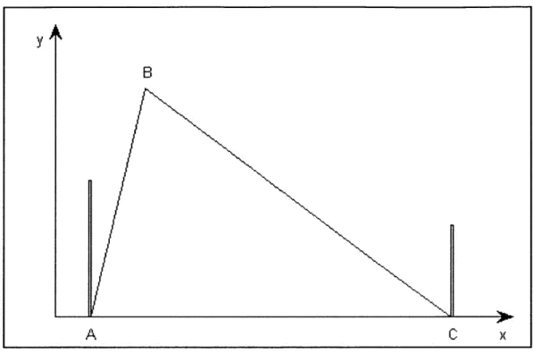
The DAT generate lognormal distribution functions in a somewhat unique manner, designed to be useful to project managers while reducing the computational costs that come from using the method: it uses a minimum value, a modal value, a maxi-mum value, and a probability that the distribution exceeds this maximaxi-mum value (See Figure 2-15).
2.3
Using the DAT in a Well Drilling Context
2.3.1
Areas and Zones
Areas and zones serve as the basic structure around which ground parameter values are generated. In their treatment of areas and zones. users should define the entire well length as a single area, and then designate zones as needed to help define the probability distribution of ground parameters- if there is any sort of discontinuity
Figure 2-15: The Lognormal Distribution Function. It is parametrized by A) a min-imum value, B) a modal value. C) a maxmin-imum value, and a probability of exceeding the maximum value.
or shift in the probabilistic distribution of a ground parameter, designate a zone to distinguish between the regions before and after that breakpoint. The appropriateness of the three different zone length determination methods (by Length, End Position, or Length AND End Position) is dependent on where the user believes these breakpoints will occurs and/or how their occurrence is probabilistically defined.
2.3.2
Ground Parameter Sets and Ground Classes
In using ground parameters, the user has three main options: use ground parameters to define rock properties (strength, abrasiveness, porosity, etc), to define lithology (gneiss, schist, etc), or to create lexicographical sets of ground types (good, bad, nor-mal, etc). The upside of using the parameters to define rock properties is that the translation of these properties into project costs and delays is direct. The downside is that the distributions of rock properties are not independently random, and so care must be given in the ground parameter generation stage. Conversely, using rock lithology offers a somewhat easier parameter generation problem, but a more difficult
translation from ground class to activity cost and schedules. Using a lexicographical ground parameter set attempts to remove the difficulties inherent in both problems
by abstracting out geological detail while retaining the ultimate functionality of the
geology section of the DAT, which is to aid in generating final cost and time distri-butions. Each of the three methods has strengths and weaknesses, and the choice between them largely depends on the information available to the modeler. What is important is to adopt a mutually exclusive, collectively exhaustive approach to ground parameter generation. Some relevant parameters, like overpressure. are often inde-pendent of rock properties or lithology, and so can be defined separately, regardless of the choice made between the three major parameter organization schemes.
2.3.3
The Well Network
The well network input is relatively straigt-forward. For most wells. construction will
the well network is often linear.
2.3.4
Methods, Geometry, and Method Selection
Method selection is the first major avenue for introducing variation into a DAT model. As the input of methods can be time intensive, the user should try to use as few meth-ods as possible while retaining desired features. Also, because method development is time intensive, the user should organize his modeling approach so as to make use of the method copying feature as frequently as possible- any activities, method vari-ables, well networks, or other components of a method that are common across the set of methods that a user plans on creating, should be created once in a baseline method, and then the development of other methods can begin from copies of that baseline method.
Well geometry, while also useful as a feature that defines methods on the basis of a well bore profile, should be more generally used to delineate methods that are different, despite sharing the same ground class- for example, a well logging stage can be given a different geometry than a well casing stage- even though the two construc-tion stages utilize the same wellbore, designating logging as one type of geometry and casing as another can make it easier for the user to specify that both a logging and a casing stage will occur across a particular well segment, even though both are being performed over geologically identical sections.
The user has two main options when it comes to method selection- one option is to define methods deterministically from geometry and ground class, while the other is to define methods probabilistically, with a pairwise combination of geometry and ground class potentially leading to more than one method. Neither approach is invalid, however it is more straightforward to keep method selection as a deterministic process, and define all uncertainty either within the ground class generation process or the method and general variable generation processes. By limiting uncertainty to these domains, the model is more transparent, and allows a user to view all of the model variability on a smaller number of program windows. When probabilistic method definition is used, it should be used sparingly, for example as a minor aid to the
ground class generation process, and certainly not utilized so as to take responsibility for generating variability from both ground class generation and parameter generation at the same time.
2.3.5
Activities
It is important to define activities in parallel with activity networks. Because the activities in an activity network are selected using a dropdown menu, it is easier to select activities that appear at the extremes of the menu, rather than its middle. Creating all of the activities in a model, and only afterward creating all of the activity networks makes the user interface more challenging to work with, as it requires the modeler to frequently search for activities within the dropdown menu rather than scroll to them instantly. Figure 2-11 demonstrates this phenomenon.
As a strictly top-down exercise, it is useful to think of activities as relating directly to physical actions taken during the construction process. A typical activity network will consist of drilling, logging, casing, and other activities. However, while this convention is wise as a general rule of thumb, it need not be followed strictly. In particular, the user may find it easier to define activities that do not have a direct relation to the construction project. This could be done either as a way of reducing the amount of user input necessary to build a model, or as a creative way of representing uncertainty. These activities can be used to add cost and schedule terms that cannot easily be associated with physical processes, or otherwise just make it easier for the user to obtain the cost and time distribution shape that is desired. Figure 2-16 shows one potential such activity, dealing with project risk due to exchange rate fluctuations.
2.3.6
General and Method Variables
Experience with construction projects suggests that lognormal distributions are par-ticularly well suited to cost representation, while triangular distributions are good approximations of schedule requirements. It is up to the modeler to decide which
dis-File View Simulation Output Help
Activities
Nc'b Na> TeE tkC tE an orAdd (I/ elete ' DelotrcAl
Nb I Nna. I Tim lwqaain - cstup~ F owof enm~ Retone~
comng
Activity
1/1-Activity Name: Currency Risk Method Variables
R skVolume Well tr ing -1000.00 0.00 11000.00 000
Heads
WellV Nn Hea4 1 1,00
General Varables:
Nit flue Oe
~
. Max.N~ ProbWej Pea MasResources:
Nb !Resource I Varbl* TV06 I Det.Vaklue Min Mode Maxr1 Probi
.Insert / - __ Resource Equations
Amount Used
Amount Produced
-Time Equation = 0 Cost Equation = RiskVolume
Priority: Preemptive: Calendar None
Figure 2-16: Activities Do Not Need to Directly Relate to Construction Processes. Here is a simple activity a user could input into the DAT to account for risk due to exchange rate fluctuations., with the potential for a $1000 reduction in costs if

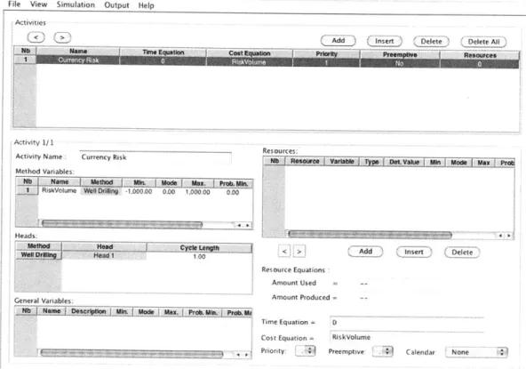
![Figure 3-2: Figure 6.9 from the Tester report [Tester et al, 2006]; a high-level break- break-down of well project costs by well depth](https://thumb-eu.123doks.com/thumbv2/123doknet/14670076.556583/50.918.172.752.124.488/figure-figure-tester-report-tester-level-break-project.webp)