Decomposition analysis of a deterministic, multi-part-type, multiple-failure-mode production line

Multiple-Part-Type, Multiple-Failure-Mode

Production Line

by

Diego A. Syrowicz

B.S. in Electrical Engineering and Computer Science, MIT (1998)

B.S.

_{in Management Science, MIT (1998)}

Submitted to the Department of Electrical Engineering and

Computer Science

in partial fulfillment of the requirements for the degree of

Master of Engineering in Electrical Engineering and Computer

Science

at the MASSACHU INSTITUTE

GY

MASSACHUSETTS INSTITUTE OF TECHNOLO

May 1999

*

~ pp PP, LIBRARIES

©

Diego A. Syrowicz,

CMXCIX.

11 rights reserved.

The author hereby grants to MIT permission to reproduce and

distribute publicly paper and electronic copies of this thesis

document in whole or in part.

A uthor ...

Department of Electrical Engineering and Cdi puer Science

May 17, 1999

Certified by...

.

Stanley

B.

Gershwin

Senior Research Scientist

Thsis Supervisor

Accepted by ...

...

. ... ...

Arthur C. Smith

Chairman, Department Committee on Graduate Students

Decomposition Analysis of a Deterministic,

Multiple-Part-Type, Multiple-Failure-Mode Production

Line

by

Diego A. Syrowicz

Submitted to the Department of Electrical Engineering and Computer Science on May 17, 1999, in partial fulfillment of the

requirements for the degree of

Master of Engineering in Electrical Engineering and Computer Science

Abstract

This thesis proposes an analytic decomposition approximation to estimate the through-put and buffer level of two-part-type flow lines with deterministic processing times and homogeneous buffers. Machines are allowed to have multiple failure modes. Machines operate according to a priority rule, processing higher priority part-types whenever possible. Machines operate on lower priority part-types only when unable to operate on higher priority parts due to either starvation or blockage. The proposed method decomposes the line into a set of two-machine-lines. Two different two-machine lines are described, one for the higher priority part-type, the other for the lower priority part-type. The solutions to the individual two-machine-lines, in combination with the decomposition relationships among those two-machine-lines, yield the analytic approximation to the performance metrics of the line.

Thesis Supervisor: Stanley B. Gershwin Title: Senior Research Scientist

This thesis was supported by many sources. First, and most important, I wish to thank my wonderful family. To my dad and mom, who never ceased to encourage me to pursue and achieve everything I desired, who were there for me unconditionally, and who helped me in every way they could. To my brother Gabriel, who was always willing to visit me, and who kept me up by telling me the good news about home. To my sister Valerie, who always looked forward to keep me company through the phone on weekends, and who never failed to sing to me. And finally, to my grandparents, Shilem, Alicia and Sofia, for always supporting me and showing me their love. To all of them, this thesis is dedicated.

From MIT academia, primarily, I would like to thank my advisor Stanley Gersh-win, who supported me technically, financially, and emotionally throughout the pro-cess of writing this thesis. He kept me going, helped me up from the hundreds of times I thought there was no way to make things work, and never let me give up. A special thanks to Prof. Gerald L. Wilson, for the plentiful advice and guidance, the lunches, Thanksgiving dinners, and most important, for his friendship.

Finally, I would like to thank my friends. I thank them for being such good friends, for sticking with me in all good times and bad. For the trips we took, the laughs, the

classes, and most important, for being who they are.

Contents

1 Introduction 7

1.1 M otivation . . . . 7

1.2 Literature Review . . . . 8

1.2.1 Single-class transfer lines with single-failure-modes . . . . 8

1.2.2 Single-class transfer lines with multiple-failure-modes . . . . . 9

1.2.3 Multiple-class transfer lines with single-failure-modes . . . . . 11

1.3 Multiple-class-type, Multiple-failure-mode transfer lines . . . . 12

2 Decomposition Derivation 13 2.1 Introduction . . . . 13

2.2 N otation . . . . 13

2.3 Part 1 Decomposition . . . . 15

2.3.1 New Events in the Part-i Two-Machine-Line . . . . 15

2.3.2 Calculation of Idleness Failure Probability . . . . 18

2.3.3 Probability of Change of Failure-Mode . . . . 19

2.3.4 Calculation of p and r . . . . 23

2.4 Part 2 Decomposition . . . . 26

2.4.1 Observable Part-2 Events . . . . 27

2.4.2 Two-Machine Line Model and Parameters . . . . 29

2.4.3 Solution Cycle for Part 2 . . . . 31

3 Part-1 Two-Machine Line 34 3.1 Introduction . . . . 34

3.3 Performance Measures . . . .

3.4 Internal State Space . . . . 39

3.5 Boundary States . . . . 47

3.5.1 Solution Technique for Boundary Equations . . . . 50

4 Part-2 Two-Machine Line 70 4.1 Introduction . . . . 70

4.2 N otation . . . . 70

4.3 Performance Measures . . . . 72

4.4 Internal Transition Equations . . . . 73

4.5 Boundary States . . . . 77

4.5.1 Solution to Boundary State Equations . . . . 79

5 Conclusions and New Research 81 A Lower Boundary PT(state) 83 B Part-2 Two-Machine-Line (z

$

0) 89 B .1 M otivation . . . . 89

B .2 N otation . . . . 89

B.3 Internal States . . . . 90

B.4 Boundary States . . . . 95

B.4.1 Solution to Boundary State Equations . . . . 101

List of Figures

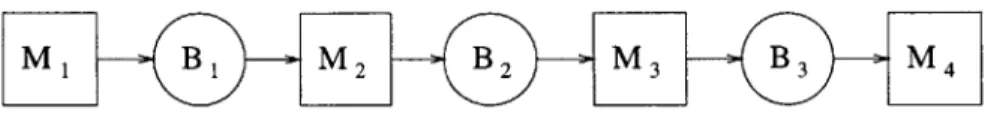
1-1 Generic Single-Class Transfer Line with Single-Failure-Modes . . . . . 8

1-2 Two-Machine-Line Decomposition Component . . . . 9

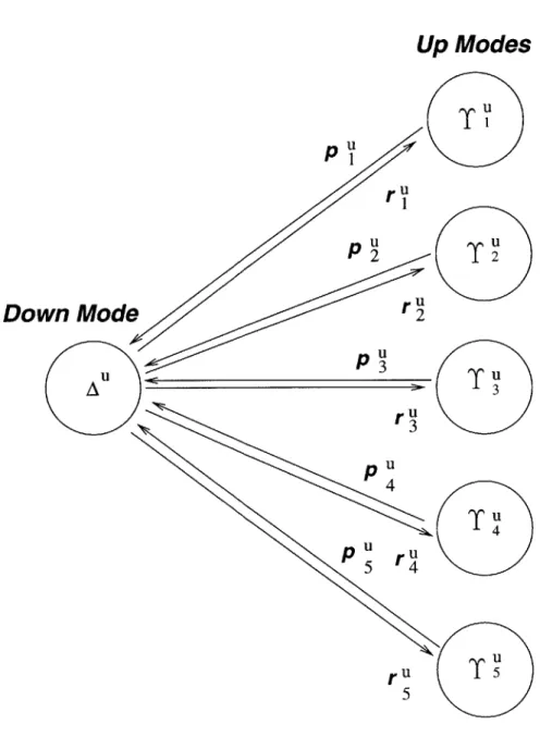
1-3 Singe-Part-Type, Multiple-Failure-Mode Two-Machine-Line . . . . 10

1-4 Multiple-Part-Type Line . . . . 11

2-1 Decomposition for typical two-part-type line . . . . 14

2-2 Ideal Machine Model for Typical M'(4, 2) . . . . 28

3-1 State Space for Mu(5, 1) . . . . 35

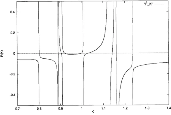
3-2 F(K) for a two-machine line with nine down modes. . . . . 45

4-1 State Space for Mu(6,2) . . . . 71

Introduction

1.1

Motivation

The design, operation, and evaluation of production lines are essential parts of the study of manufacturing systems. Most of the fieldwork is done through computer simulation of the stochastic processes underlying the production flow line. However, simulations require a considerable time commitment to construct and run. Recent work done by Gershwin [12] suggests that it is possible to construct a closed mulation of production lines under various operational assumptions. Current for-mulations developed include those with single-class single-failure-mode determinis-tic behavior lines [12], single-class single-failure-mode continuous behavior lines [14], single-class multiple-failure-mode deterministic behavior lines [19], and multiple-class single-failure-mode deterministic behavior lines [17]. These formulations usually yield solutions that approximate the solutions of the simulation without the required com-putational power and time. This thesis constructs a formulation for a production line under deterministic, multiple-part-type, multiple-failure-mode assumptions.

CHAPTER 1. INTRODUCTION

M B M 2 MB

Figure 1-1: Generic Single-Class Transfer Line with Single-Failure-Modes

1.2

Literature Review

1.2.1

Single-class transfer lines with single-failure-modes

A transfer line is a production system whose work proceeds in a linear fashion from

one machine to the next. A single-class line is one in which the transfer line only builds one type of part. An example of a single-class flow line is depicted in Figure

(1-1). A flow line has machines (M) which perform some work in a part, and such are

depicted by the squares in the figure. Parts flow from machines into buffers (B), or storage centers, which are depicted by circles. The arrows that connect the machines and buffers represent the path of work-in-process, and the direction is from left to right.

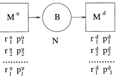
One way to analyze flow lines is to break them into simpler structures, specifically, two-machine-lines. This is the technique called decomposition. Once a formulation and solution to the two-machine-line is found, it may be possible to find an approxi-mate solution to the complete flow line. A two-machine-line is depicted in Figure 1-2. In order to solve a two-machine-line, it is necessary to have a behavior assumption and a representation of the machines and the production process. The representation requires the size of the buffer (N), the failure rate of the machines (p), the repair rates (r), _{and the processing rates (p).}

The simplest characterization of the production flow is the deterministic model. Under a deterministic assumption, the processing rates of all machines are constant. A machine processes one part, in one time unit, asynchronously from other machines. In addition, a machine cannot process a part if it is starved (there is no available material

u

ru

pu

N

d

rd pd

Figure 1-2: Two-Machine-Line Decomposition Component

in the buffer preceding it), or it is blocked (there is no space in the buffer receiving parts from the machine). Generally, a machine is not allowed to fail unless it is working on a part. In addition, in a two-machine-line, the upstream machine is never starved (there is always raw material), and the downstream machine is never blocked (there is always space to put completed parts). The formulation and solution of the resulting deterministic two-machine-line is achieved by solving a two-dimensional Markov chain with 4(N - 1) states [12]. The solution to such a chain is given as the

steady state probability of all states, the line's buffer levels, and the overall production rate.

Through other types of assumptions and solution techniques, other process behav-iors can be captured. For example, using a continuous flow assumption, it is possible to allow for machines to have different processing rates.

1.2.2

Single-class transfer lines with multiple-failure-modes

The transfer line models discussed above assume that machines may fail only in one way. Current work done by Tolio [19] allows for a similar formulation of production lines with the added feature that a given machine may fail in one of several modes, and be repaired in the mode corresponding to the specific failure mode. Thus, for example, a machine may fail because a part got stuck, and take an average of 5 minutes to repair, or because the motor exploded, and take an average of 5 days to repair. A two-machine-line building block representation is depicted in Figure 1-3.

CHAPTER 1. INTRODUCTION

ru pu

rd

d r u PU rd d

r2p

r

2

P2

...

000 00 0 0 0.000 r!' PP d d

Figure 1-3: Singe-Part-Type, Multiple-Failure-Mode Two-Machine-Line Single-failure-mode models cannot deal directly with multiple failure modes. In order to use those models on lines with multiple failure modes, one has to first average the multiple failure and repair rates, and use the averages to represent the parameter for a single-failure-mode machine. The problem with averaging is that, for sets of considerably different failure modes, the variance cannot be captured accurately. This results in less accurate steady state solutions for the performance measures.

Another feature of multiple failure lines is that in the decomposition process, two-machine-lines can assign failure modes to account for the probability of starvation and blockage due to failures of machines outside of the two-machine-line. These failure modes are called virtual failure modes as they are not real failure modes. During decomposition, the steady state solution is reached when the convergence of the production behavior of every two-machine-line is achieved [4]. For every two-machine-line, behavior paramenters are analyzed and changed in an ordered way until convergence is achieved. By allowing a two-machine-line to account directly for new possibilities of failure, the accuracy of the solution is usually improved.

- d

.

M...u

M

ru pU

B2

N

2 rd

pd

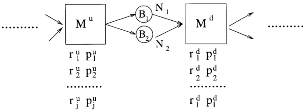
ru pU rdpd B22 r2 p2 2 r P 2 ry p, ri p

Figure 1-4: Multiple-Part-Type Line

1.2.3

Multiple-class transfer lines with single-failure-modes

Recent work conducted by Nemec [17] formulated and solved for deterministic behav-ior lines that processed more than one part type. A simple multiple-part-type line is depicted in Figure 1-4.

Because the line works on different parts, there must be a policy. Nemec describes the policy as one with priorities. Thus, part 1 is always worked on if there are parts to work with and the machines are not blocked or starved. Only if there are no part Is to work with, part 2s are started, and so on. If a higher ranking part arrives to be worked on while a machine is working on a lower ranking part, the next part to be processed will be the higher ranking part. Setup times are assumed to be zero. Buffers are homogeneous. In other words, buffers only hold parts of a single part type. Because there is a buffer for every part-type, blockage and starvation are part-dependent events.

CHAPTER 1. INTRODUCTION

1.3

Multiple-class-type, Multiple-failure-mode

trans-fer lines

Nemec formulated a deterministic single-failure multiple-class transfer line. However, this formulation only worked for small two-class-type lines. The reason why the formulation worked only in a limited set of lines is that possibly, the two-machine-lines are unable to describe accurately all the failures, blockages, and starvations possible due to other part-types and other machines.

One goal for the research of decomposition is to achieve a formulation that ac-counts for both multiple-part-types and different production speeds for each machine. Nemec's work tries to account for multiple-part-types. However, he was unsuccessful in formulating a deterministic model that could work for more than six machines and two part-types. The extension to a continuous case model (one with different process-ing speeds per machine) would prove to be difficult. The work done by Tolio suggests that there is a potential solution to the underlying problems in Nemec's model.

By using a multiple-failure-model formulation, most of the second moments in the

multiple-type line could be captured. This would increase the accuracy and decrease the complexity of the desired formulation. The first step of this thesis will be to determine the state transition dynamics of such a model. Then, a decomposition method for this type of line will be determined. Finally, the general two-machine building blocks will be constructed and analytically solved.

Decomposition Derivation

2.1

Introduction

In this chapter, a decomposition analysis of a processing line with finite homoge-neous buffers, unreliable machines, and two different part-types is presented. Like the decomposition analysis done by Nemec [17], the multiple-part-type line analysis is conducted by decomposing the line into single-part-type two-machine sections cor-responding to all real homogeneous buffers. Although the two-machine sections are part-type specific, the state transitions seen by all of these sections are interwoven with events occurring in other two-machine lines, including ones of different part type.

2.2

Notation

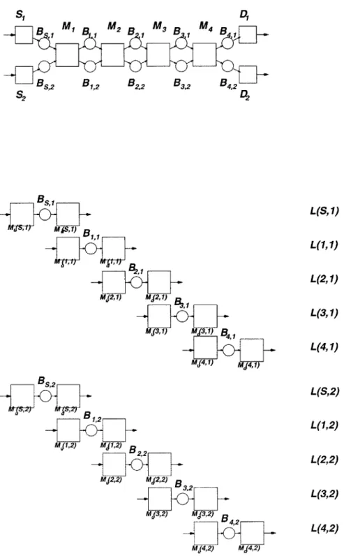
The decomposition of the two-part-type line is illustrated in Figure 2-1. The notation used to refer to items within the decomposition will follow, for the most part, the convention set by Nemec [17]. Part-specific notation must be introduced to deal with new event types contemplated by the decomposition; those will be introduced in later sections.

Machines and buffers in the decomposition are part-type specific, and therefore,

14 CHAPTER 2. DECOMPOSITION DERIVATION

S, D B, , M B, M3 B, M4 B, Bs,2 B1,2 B2,2 B3,2 B4,2 S2 2 L(S,1) ,MJS,1)B L(1,1) L(2,1) MJ2,1) MJ2,1) L(3,1) Md3,1) _{M 31)B,} --- w L (4, 1) MJ4, 1) MJ4,1 L(S,2) L(1,2) MJ1,2) Mj1,2) 822 L(2,2) MJ2,2) MJ2,2)32 L(3,2) Mj3,2) MJ3,2) |L(4,2) M4,2) MJ4,2)

unlike single part-type lines, identifiers must include a part-type index, c = {1, 2},

in order to differentiate between similar items for different part-types. In the decom-position, each buffer Bc,,, has a corresponding two-machine line, L(q, c); where r7 is the two-machine-line index number, and c the part-type. Machines corresponding to the real processing line are called real machines, whereas machines from the two-machine-lines are called pseudo-machines. The upstream pseudo-machine for L(7, c) is denoted M'(q, c); the downstream pseudo-machine is denoted Md(r,, c). The size of the real buffer Bsc is the same size as B(q, c), and is denoted N(7, c). The current buffer level of L(m, c) is denoted by n(q, c).

2.3

Part 1 Decomposition

In the real line the introduction of multiple part-types creates a more complex en-vironment than that of single part-type lines. Such added complexities must also be captured by the decomposition analysis, and, as a result, additional notation is necessary. A development of the decomposition analysis for type one parts follows. The additional notation required is described as need arises.

2.3.1

New Events in the Part-1 Two-Machine-Line

Like in the Tolio decomposition [19], pseudo-machines can suffer from real failures and virtual failures. Real failures are failures of the real machines as represented by the pseudo-machines of the two-machine-line. Virtual failures are the failures modes introduced to account for the effect that real failures outside of the two-machine-line have on the two-machine-line itself. However, the events which an observer standing in the buffer of a part-1 two-machine-line would see are more complicated than those in a single-part-type line. Sometimes, from the perspective of the observer, when a

CHAPTER 2. DECOMPOSITION DERIVATION

pseudo-machine is not allowed to work', it could still fail2_{. The new failure types are} idleness failures, and failure-mode-changes.

Idleness Failures

As in the case with the one-part-type deterministic line model, machines are pre-vented from working when they are starved or blocked. However, since buffers are homogeneous, when a real machine is starved or blocked for part 1, it is not neces-sarily blocked or starved for other part-types. Indeed, because the machine is not in any real failure mode, the it can process lower-priority part-types. While the real machine is working on such part-types, the it can fail as well. From a part-1 ob-server's perspective, this means that while the observed buffer is completely full or empty, failures that could not occur in the one-part-type case are now possible. If the originally blocked or starved pseudo-machine gets unblocked or unstarved, and it is down because of a real failure, the pseudo-machine is said to have seen an idle-ness failure of mode

j,

where

j

is the indicator of the failure mode observed. The identifier q will be used to describe such probability. Thus, for example, q' (5, 1) is said to be the probability that Mu(5, 1) fails in mode 3 when it is blocked. Notice that idleness failures in the two-machine-line context occur only when the upstream pseudo-machine is blocked, or the downstream pseudo-machine is starved.

Failure-Mode Changes

When failures are virtual, although part 1 cannot be processed by the affected real machine, it is conceivable that part 2 could be processed instead. As with idleness failures, real machines could continue working on lower priority parts while the

part-1 virtual failure is repaired. The usual scenario would be one in which the virtual

failure would be repaired while the real machine worked on lower-priority parts, and 1_{whether because it is down, or it is blocked or starved}

2_{since the machine could be doing lower priority parts}

thus it would return to working on part 1. In a similar way, even if some machine failure caused a virtual failure to the lower-priority-part production, it is conceivable that such failure would be repaired before the initiating failure was repaired. The initiating failure is defined as the failure that caused production to start for a lower-priority part-type. In such instances there would be nothing new added to what a part-1 observer would see. However, there is the possibility that the initiating failure is repaired while some other failure was felt by the observed two-machine line. In other words, this is the case that will be referred to as a failure-mode change, and will be symbolized by variable z.

The importance of failure-mode changes relies on the fact that even though the part-1 pseudo-machine will continue to be down, there would be a change in the repair probability. In order to capture this probability change, a transition probability between down modes must be specified.

It is important to notice two important observations in failure-mode changes. The first is that a failure mode change can only occur from the initiating mode to a mode corresponding to a machine which is closer to the observer's location. The reason for this is that the initiating failure corresponds to a real failure of some machine, which has propagated by means of starvation or blockages to the observer's location. A real machine under a real failure mode may not work on any part type, and thus, even if machines farther away from the observer's corresponding real machine fail, those failures will not propagate to that location unless the initiating failure is repaired. However, real failures that occur to machines closer to the observer's location than the real machine to which the initiating failure corresponds will block the effects of a repair of the initiating failure.

The other observation has to do with the timing of a failure-mode change. The situation in which a failure occurs when processing a lower-priority part is not enough to cause a failure-mode change. After all, not only must a new failure occur and the initiating failure be repaired, but also the repair of the initiating failure must

CHAPTER 2. DECOMPOSITION DERIVATION

propagate to the new failure location before the initiating failure is repaired. In other words, a failure-mode change is only said to occur after both, the initiating failure is repaired, and part-Is have propagated to the location of the new failure. If the new failure was repaired for the lower-priority parts before the full propagation occurred, the initiating failure's repair would reach the observer's location, thus eliminating the need for a failure change possibility.

Assumption 1: A failure-mode change is not experienced by an observer in the part-1 two-machine line until the initiating failure is repaired, and part-1 type parts

have propagated to the new failure's location.

2.3.2

Calculation of Idleness Failure Probability

The changes in the decomposition process with respect to Tolio's single-part-type decomposition have to do with the new failure types. The idleness failures complicate the process insofar as the boundary states are concerned. In other words, since idleness failures only occur in blockage or starvation instances (i.e. the observer's buffer is full or empty), then q's will only be seen in boundary transition events.

Because q is conditional on being at a given boundary state, the expression for

q is only contingent on the probability of a given failure type occurring. Since a

pseudo-machine could only fail if the local real machine was working on an alternative part type, q will be an expression which includes the probability of the real-machine working on the alternative part type. In other words, idleness failures only occur due to failures of the local real machines. Therefore, idleness failures only cause failures to real modes. In a two-part line, this translates into

qj(71, 1) = p (,q)P (M' (',, 2) non-idle) (2.1) and

q,(, 1) = pi(y + 1)P

(M(,

2) non-idle) (2.2) where p3 (,q) and pi (TI) are the probabilities of real failures for the real machine r7, and

the non-idleness probability can be calculated as a sum of states from the two-machine line analysis.

2.3.3

Probability of Change of Failure-Mode

A convenient way to begin to think about failure-mode changes is to study the

rela-tionship between neighboring machines which are in identical failure modes. When a failure occurs somewhere in the line, as the failure propagates through the line causing virtual failures, more than one observer will see this failure mode. Because all intermediate buffers for part-1 would empty out as the virtual failure propagates downstream, then mode changes propagate as well. In fact, when a failure-mode change is experienced by an observer, all the observers which were in the same failure mode will simultaneously experience it too. The reason for this behavior relies in the fact that all part-1 buffers are empty between the initiating failure location and any observer who has felt the failure. Thus, if any of the observers has seen a failure mode change, since all buffers between his location and any observer in the initiating failure mode are still empty, all observers see the same failure type.

zL,, (, +1,1) = zj, (T, 1) , for j' < j, (2.3)

and

Zi - 1,1) = z( 1) , for 1' > 1, (2.4)

where j' and ' refer to the initiating failure modes, and j and 1 refer to the mode to which a transition occurred.

CHAPTER 2. DECOMPOSITION DERIVATION

Because of (2.3), it is only necessary to calculate zjj(rq 1) for the machine rq to which mode

j

belongs. The complexity of calculating this probability increases as the separation between

j'

and

j

increases.

The simplest case is when

j'

and

j

refer to adjacent real machines. For example, if for simplicity we assume that mode numbers correspond to specific machines3, z3,4(4, 1) would refer to the probability that the observer in L(4, 1) sees a failure

mode change from failure mode 3 to failure mode 4. More specifically, in the case of a two-part line, z34(4, 1) means that the following events happened in order (from

that observer's point of view):

1. A virtual failure of type three occurred in Mu(4, 1) while working type 1 parts.

2. Although Mu(4, 1) is virtually down, M4 is not truly down and can work on

type 2 parts.

3. While making type two parts, M4 fails.

4. M3 got repaired while M4 was still down.

The moment that M3 gets repaired, a part is put in B(3, 1). Following with

Assumption 1, if Mu(4, 1) was not repaired at the same time, this immediately means that a change of failure from mode 3 to mode 4 was experienced by the observer.

The probability calculation for zg4(4, 1) is dependent on failure-mode 3 having

been experienced by M4. Thus, the calculation reduces to the probability of any of

the following events occurring:

" Mu(4, 1) fails and M3 gets repaired at the same time.

" M'(4, 1) fails, and after one time step, M3 gets repaired but Mu(4, 1) is not

repaired.

3

which would also imply that each machine has only one failure mode.

* M"(4, 1) fails, after one time step neither M3 nor M'(4, 1) gets repaired, and

after two time steps M3 gets repaired and M"(4, 1) is not repaired.

* Muu(4, 1) fails, after s - 1 time steps neither M3 nor Mu(4, 1) gets repaired, and after s time steps M3 gets repaired and Mu(4, 1) is not repaired.

Before calculating the probability corresponding to such events, a simplifying as-sumption must be made. Specifically, that after an originating failure occurs, part-2 would start to be processed, and work on part-2 would not be starved or blocked on

M4.

Assumption 2: Once an originating failure occurs, part-2 is processed by the

line without interruption unless there is another failure, or the initiating failure is repaired

What Assumption 2 means is that the probability that pseudo-machines are idle for part-2 do not have to be calculated. This assumption may be justified by the fact that one is most interested in evaluating the performance of lines that have limited capacity. Thus, in a two-part line, if there is overwhelming capacity, all demand would be satisfied easily. However, if capacity is limited, part-1 would usually be the one being processed, and when there was an opportunity to work on part-2, it would rarely be the case that the machine would not be able allowed to do so because of starvation or blockage.

Given Assumption 2, the calculation reduces to the sum of all the aforesaid events:

z3,4(4, 1) =p4r3 + P4(1 - r3)(1 - r4)r3 +.. 00 = p4r3 Z[(1 - r3)(1 - r4))s s=O p4r3 1 - (1 - r3)(1 - r4)

CHAPTER 2. DECOMPOSITION DERIVATION Generalizing, z _-'(i j U 1) =j_{1) 1} -(1 - rj_1)(1 - rj) Using (2.3), z_1,( _j1- 1 ₍₁ (1-=1 _{- rj_1) (1 - ry)} , for r; >

j.

(2.5)

The calculation of zj,,j(r/, 1) for

j

>

j'

+ 1 is harder because as the separation

between real machines increases, there are increasingly more event-sequences through which a change of failure mode is possible. In order to calculate this quantity, another simplifying assumption must be made: that once a machine is in originating failure mode

j',

all machines between

j'

and

j

are up. The reason why this is an acceptable assumption is that if the real machines between

j'

and

j

were down, or allowed to fail and then be repaired before the transition from

j'

to

j

occurs, the probability contribution would be comparatively small. Machines which start down between

j'

and

j

must be repaired before the effects of the repair of

j'

reaches them. If this was not the case, then the failure-mode change would not be from

j'

to

j,

but from

j'

to some

j"

<

j.

However, this repair would require a repair probability factor, which would make the probability contribution smaller. Similarly, terms which include failures of machines between

j'

and

j

will not be included as otherwise not only would the failure probability need be included as a factor, but also its corresponding repair probability.

Assumption 3: In calculating the failure-mode change probability from

j'

to

j,

all machines between

j'

and

j

are assumed to be up. In addition, terms requiring failures of real machines between

j'

and

j

will be ignored as their probability contribution is minimal.

Using Assumption 3 and equation (2.3), it can be shown that

pyry(1 - rj)-'- HI' ₁ (1 - p₁)lj'+1

ziu, i (r, 1)) =j fj_1 (2.6) 1-(1 - r 1- r) H +1( ~ Pv)

for rj > j, and j' < j.

Note that, following the convention of single failure modes per machine, j's refer to both failure mode type, and machine number. In the case that multiple failure modes exist for machines, quantities like

j

-

j'

must be expressed in terms of machine numbers.

A similar process for the downstream pseudo-machine yields

d pirj+1 +1,l 1)= 1 - (1 - rj+₁)(1 - ri) Using (2.4), d pITl+1 zl+ d ZllI'l (rj, 1) 1)=1 - (1 - ri+)(1 - rj)(27 (2.7) and piri,(1 - rH _-1+1( - Ph) .+1

1 - (1 - r - ri) hi)(1 Ho-j+1(1 - P )

for 1 > 7, and 1' > 1.

2.3.4

Calculation of

p

and r

The decomposition derivation for p and r follow the methodology line of Tolio's decomposition [19], but for a few modifications to the equations. Once again, notation must be slightly modified to accommodate the fact that there are two part types.

CHAPTER 2. DECOMPOSITION DERIVATION

Notation Summary for Decomposition

The required notation for the upstream pseudo-machine is

WU(r,, 1) The probability that machine M"(77, 1) is operating on a part.

D'(7, 1) The probability that machine M'(r,, 1) is down with real failure mode

f.

X(,f)( 1) The probability that machine M'(, 1) is down with virtual failure mode

(j,

f),

where

f

refers to the real failure mode of initiating machine

j

(upstream from q).

P(j,f)(,7, 1) The probability that machine Md(, 1) is starved due to failure

f

from initiating machine

j

(upstream from q).

E(i, 1) The efficiency of two-machine line (IJ,1).

Decomposition Derivation of p and r

Wu(r,, 1), the probability that Mu(iq, 1) is working on a part, is simply E(q, 1). The reason for this is that the upstream pseudo-machine in the two-machine line cannot be starved, and thus it will always be working on a part when it is not down or blocked.

Wu( 7, 1) = E(rl, 1) (2.9)

Virtual failures are introduced to mimic the effects of failures of non-local real machines in the two-machine line. The effects of such failures propagate as starva-tions or blockages. Therefore, it must be the case that there is a correspondence between virtual failures and starvations/blockages in neighboring two-machine lines. More specifically, the probability of a virtual failure in Mu(r,, 1) starting at time t,

X",f)(mr, 1), must be equal to the probability of starvation of Mu(j - 1) starting at

time t, Ps(Jf)(7 -

X,)(r , 1) P8(Jf)(Tl - 1, 1) (2.10)

The frequency of entering into a virtual failure mode must be equal to the fre-quency of leaving it. Essentially there are two ways in which a virtual failure mode could be entered or exited: (1) by real failures/repairs, and (2) by changes in failure-modes. In the context of virtual failure modes, this translates into:

X(jj,f)(rl, 1) rLf)(rl, 1) +

E

zQf),(Jf( 1)

W"(r, 1)p",f(r, 1) +

E

X(,f)"(r/, 1)z, (, 1) (j,f)"

where the sum

E(j,f)I

z(,f),(jf)/ is over

(j,

f)'

>

(j,

f).

In other words, mode

(j, f)'

corresponds to a real machine closer to r/ than

(j, f).

The sum

Eujfr

is over

(j, f)"

<

(j,

f),

i.e.

(j, f)"

is mode corresponding to a real machine farther away from r than

(j, f).

Introducing the notation fu(r 7,1) as representing the sum of all probabilities of

leaving down state (j,

f):

USf)(r/, 1) = rjf)(r/, 1) + Z(j,f),(jf)1(i7/ 1), (jlf)' >(jf) then, X(,f) 1,)(r, 1) = W"(r7, 1)pgf(r0, 1) + X(jf)"(r0, 1)z(,f/,(j,f)(m 1) (j,f)" Using (2.9) and (2.10),

DECOMPOSITION DERIVATION

PS(J,f) (r) - 1, 1)f)(m, 1) = E(r, 1)p",f(, 1) +

Z

(U,/)"

Re-arranging terms,

P(j,f) (7 1

U(f)(97, 1)Ps(y,f)(r - 1,1) -

E(j,f)

Ps(j,f)y(r - 1, 1) z,fy,(yf)(r, 1)

E(7,71)

(2.11) Since

(2.12)

E(1, 1) = E(2, 1) =...=E(7, 1) ... =E(m, 1)

then by (2.11) and (2.12) f 1 f)(1, 1)Ps(j,f)(7 - 1, P(j ,/) 07 1 1) - Z~~f yPs(,f)(r - 1, 1)z(,Uf),(,f)(m' 1) E - 1,1) (2.13)

Using a similar method and notation, pf(r/, 1) is found to be

pd ,f)(r/ 1) =

if(r, 1)Pb(j,f)(7 + 1, 1) - E(j,f)' Pb(j,f)y (rq + 1, 1)z yf),Jf(r, 1)

E(r + 1, 1)

(2.14)

2.4

Part 2 Decomposition

This section develops the decomposition analysis for the part 2 behavior. Part 2 is the part with the lowest processing priority, and machines in the real line will only work on such part-type when blocked or starved for the higher priority part-types. For notation reasons, a part c realm for a given machine or two-machine line will be

CH APT ER 2. 26

defined as the space in time when such machine or two-machine line is allowed to work on part-type c (c = {1, 2}).

2.4.1

Observable Part-2 Events

Part-2 observers see a different event space than the one seen by those standing in part-1 buffers. Since working on part 2 only occurs because a virtual failure occurred for some machine in the part-1 realm, then there are different ways in which part 2 production could start. This is important because the failure type which occurred in the part-1 realm (the initiating failure), determines the way in which the production in the part-2 realm could fail. Thus, for example, if M'(5, 2) started production because of initiating failure mode 3 (M3 failed), then Mu(5, 2) can only fail if either

" M3 is repaired and Mu(5, 1) is repaired from the corresponding virtual failure. " M'(5, 2) fails in virtual mode 4 (i.e., due to the failure of M4).

However, if Mu(5, 2) entered production because of initiating failure mode 1, then

Mu(5, 2) can fail if

" M1 is repaired and Mu(5, 1) is repaired from the corresponding virtual failure.

" Mu(5, 2) fails in virtual mode 4.

" Mu(5, 2) fails in virtual mode 3.

" M"(5, 2) fails in virtual mode 2.

Thus, there are various up-states needed to have the memory required to account for the different failure modes corresponding to each initiating failure mode.

The ideal part-2 machine model would require new states to differentiate between the different down-modes on which part-2 could be. Indeed, each up state would have down states which correspond to identical failure modes. The reason for the different

CHAPTER 2. DECOMPOSITION DERIVATION

Doing Part 1

Doing Part 2 Due to virtual

Failure j in Part-i Realm

Down States (Part-2 Realm)

Figure 2-2: Ideal Machine Model for Typical M'(4, 2)

down-states is that when a virtual failure occurs in the part-2 realm, such could be repaired before the initiating failure. Because a virtual failure for a given up-mode could only return to doing part 2 in that same up-mode (or simply fail into doing part-1), then such down-mode could not be shared by multiple up-modes. Figure 2-2 depicts the ideal pseudo-machine model for part 2.

Unlike part-1 observers, part-2 observers would not see idleness failures. In addi-tion, there would not be changes in failure mode since part 2 is the lowest priority part, and on blockage or starvation no other part would be processed. Because the set of possible states is extremely complex, simplification is necessary.

Simplifications

Several solvable models could be devised to capture some part of the behavior of part 2. Each model would sacrifice different details and events. The choice of model is hard, especially without apriori knowledge on what events are most important.

The simplification that is pursued here is one in which, for every pseudo-machine,

-C

(n e

SOJ

there are multiple up-modes and one down-mode. Some of the reasons why such model seems reasonable are:

* It is more likely that after the initiating failure occurs, if a virtual failure occurs

in the part-2 realm right after, the initiating failure will be repaired before the virtual failure does. Therefore, the required state transition in the part-2 realm would be from a virtual down mode to the down doing type one parts down mode. Thus, down states specific to each up mode are usually not required.

* Even with no up-state-specific failures, multiple up-modes will allow to have

different probabilities of failing. Such probabilities could be adjusted to include all the different ways in which a failure could occur. Similarly the ways in which the up-mode could be entered could be adjusted to include intermediate failures. A multiple-down-mode model would not allow for a similar calculation to be done to adjust for the multiple up-state behavior.

The approximation is usually a realistic one in lines with similar machines. Po-tentially problematic cases would be the ones with machines which fail very often (in comparison to others in the line). However, if a machine fails and it is repaired very often, then its effects would usually not propagate to be felt as virtual failures. Also, if the machine failed very often, and was repaired slowly (comparatively speaking) then the whole analysis would be almost useless as the problems in production are due to that very unreliable machine.

2.4.2

Two-Machine Line Model and Parameters

The two-machine line model that will be used will thus be the one with multiple up-modes and one down-mode. In addition, there will neither be idleness-failures, nor up-mode change probabilities.

The complication with the model comes about from the fact that the line is to process part 2. To find the needed parameters

(r's

and p's) several assumptions and

CHAPTER 2. DECOMPOSITION DERIVATION

calculations must be performed.

Symmetry of p3(r/q, 1) and r,(q, 2)

In order to calculate rl(r/, 2) one must first recall the reasons why M, would do part 2. part 2 is processed by M because, in the part-1 realm, Mu(r,, 1) went into some virtual failure. Thus, the probability of M starting to process part 2 is at least the same as the probability that the initiating failure occurred. The probability could be larger if adjustments were to be made to account for the fact that once in an up-mode, a virtual failure could occur and been repaired before the initiating failure was repaired. For simplification reasons, and since this was the original simplification motivation in the choice of the model, such probabilities will be ignored. Thus:

ri (rl, 2) =pj (, 1) (2.15)

and

rf'(r/, 2) = p'(r, 1) (2.16)

where the upstream-machine's down-mode

j

in part 1 corresponds to the same real mode as up-mode i in part 2, and equivalently between modes

f

and 1 for the down-stream pseudo-machine.

Calculation of py (r7, 2) and pd(r/, 2)

The calculation of failure probabilities in part 2 pose a harder problem than the repair probability. A failure from a given upstate could occur because the initiating failure was repaired, or because another failure was felt within the part-2 production realm. This quantity will be solved by finding relationships between neighboring two-machine lines. It is noteworthy to mention, however, that such probability should be some function of the repair probability for the initiating machine failure.

2.4.3

Solution Cycle for Part 2

The decomposition process for part 2 cannot follow the Tolio's decomposition method exactly since the problem presented must deal with issues of multiple up-states instead of multiple down-states, in addition to incorporating part-1 events. The only variables that remain to be found for use in the two-machine lines are: p,"(rq, 2), the probability that Mu(T, 2) fails while in in up-mode i, and p'(, 2), the probability that Md(r, 2) fails while in up-mode

j.

There are three components that come into play in such probabilities; looking into p"(r, 2) they are:

1. The probability that the initiating failure

j

was repaired for Mu(rq, 1)

2. The probability that a real failure occurs to M while it is working on part 2

3. The probability that a Mu

(rI,

2) experiences a virtual failure by means of star-vation

The first component, the probability of the repair of the initiating failure, is rj(r/),

which is the r for the real machine to which

j

belongs.

The second component, a real failure of M, while it is working on part 2, is also related to the real failure parameters of that machine. Given that the real machine is in the part-2 realm, and it is in up-state i, it can only fail if it is not starved or blocked (i.e., working on a part). Thus the probability of that happening is just the sum of all the probabilities of real failure

E

I p9(r/) (where G is the number of real

failures for machine rn) times the probability of that MU(rI, 2) is non-idle.

The final component can be related to failures (virtual or real) in the upstream neighboring two-machine-line. In order for these failures to be felt by Mu(i, 2), prop-agation by means of starvation must occur. Thus, looking at virtual failures for the upstream machine Mu(r/, 2), where the i symbolizes that the machine is in up mode i, a virtual failure occurs after either:

DECOMPOSITION DERIVATION

" M"(* - 1, 2) is in mode i and fails while B(r7, 2) = 0, and M '(q, 2) does not

fail.

" M"(7 - 1, 2) is down and B(r/ - 1, 2) = 1, and Mi (7, 2) does not fail.

Defining

Wu'0 (7j - 1, 2, i) The probability that Mu(r/ - 1, 2) is up in mode i, and B(n - 1, 2)

has zero parts in it

Du'1 (T - 1, 2) The probability that MU (r - 1, 2) is down and B (q - 1, 2) has only one

part in it

where both terms can be calculated by the sum of probabilities of states in the two-machine lines, and defining PM(q) as the sum of the probabilities of all possible real failure types for M(7),

G

PM (7) E pg (7),

g=1

then, adding the probabilities for the aforesaid components:

pu (r), 2) = rg (r,1) + PM(r)

+ (1 Pu~r)) W'0 (r/ - 1, 2, iOpu (r/ - 1, 2)

+ (1 - Pm(r7)) Du'1(,q - 1, 2)

(1

_-

E

alli'

(2.17)

where mode i in part-2 pseudo-machines is equivalent to mode

j

in part-1 pseudo-machines.

32

CH APT ER 2.

Following a similar methodology for the downstream machine,

p'(rl, 2) = 1) + Pm(r + 1)

+(1 - PM(r/ + 1)) W(2) + 2, + 2) 1pd)

+ (1 - Pm(r/ + 1)) D d' (r/ + 1, 2) 1 -

E

rdj, (r/ + 1, 2) (2.18)

Chapter 3

Part-1 Two-Machine Line

3.1

Introduction

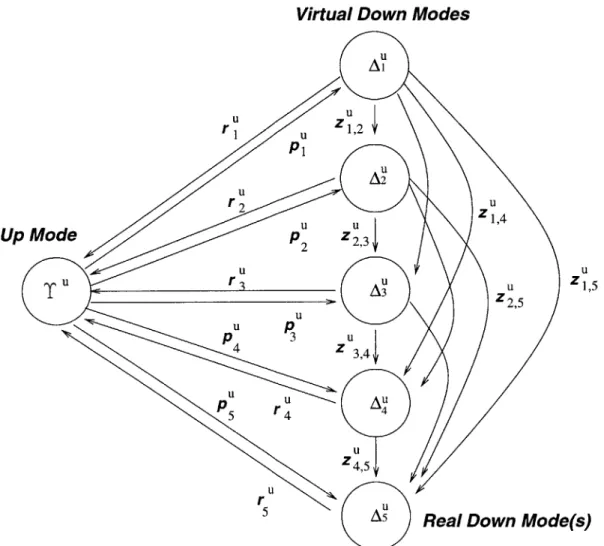
This chapter presents the solution technique for the two-machine line chosen to rep-resent the behavior of part 1. As discussed in Chapter 2, in order to analyze a long line it is necessary to decompose it into two-machine-lines. The Markovian model chosen for part 1 is one similar to Tolio's model [18] insofar as having one up-mode and multiple down-modes. However, because of changes in failure mode, it is now possible to go from a given down-mode to other down-modes. In addition, the intro-duction of idleness failures will further make the the solution technique differ at the boundary states.

Figure 3-1 depicts the transition space for a typical upstream machine in the two-machine line.

The introduction of changes of failure mode creates several conceptual and math-ematical problems in the solution method pursued. Because of this difficulty, this chapter concentrates in developing the model that introduces idleness failures into the part-1 two-machine-line. The work done with the introduction of changes in failure mode is presented in Appendix B.

Virtual Down Modes U Al U zi2U r u zu,2 P1 U A2 UU r u zu Z1

i,

4 Up Mode pu z 2,, Suu u T Ur U 1,

Real Down Mode(s)

CHAPTER 3. PART-1 TWO-MACHINE LINE

3.2

Notation

The notation used will follow as much as possible that defined by Tolio [18]. A' represents down mode

j

for the upstream machine, and Ad represents down mode 1 for the downstream machine. Because there is only one up state for each machine, T"

and Td represent the up states of the upstream and downstream machines respectively. Probabilities of repair or failure are still represented by r, r p, and p. New notation is introduced because of failure mode changes. A probability expressed as z", represents the probability of the upstream machine having a change from down mode t to down mode

j.

The expression z,1 represents the probability that the downstream

machine has a change from down mode x to down mode 1. Since this chapter will assume that there are no failure mode changes, all z's will be defined to be zero.

The expressions for idleness failures is represented by the letter q. Thus, qj is the probability that the upstream machine has an idleness failure, and went into failure mode

j,

Ay.

Defining a* (t) as the state (up state or down state) of a machine * at time t (where

* is either upstream or downstream), then we can define r, p, q, and z as

r = prob(au(t + 1) = TI a"(t) Au)

= prob(ad(t + 1) = Td ad(t) = Ad)

p = prob(au(t + 1) = aI a(t) = Tu and n(t) < N)

p = prob(ad(t + 1) =Ad ad(t) =T and n(t) > 0)

q = prob(a"(t + 1) = AU I au(t) = Tu and n(t) = N)

q = _qf prob(ad(t + 1) = Ad ad(t) =T and n(t) = 0) f

= prob(a"(t + 1) = A,/ a"(t) = A')

zly _{prob(1(t +1) = Ad| ad(t) Ad}

For any given down mode, fj for the upstream machine, or fd for the downstream machine, will represent the probability of leaving a down mode. Because a down state can be left via repair or failure change, fj is the sum of the probabilities of all such possible events. J t=j+1 and l-1 fdr + L x=1

Since all z's are zero, i reduces to r.

Similar to Tolio's method [18], Pu and Pd are J j=1 and L pd d 1=1

where J and L are the total number of failure modes for the upstream machine and downstream machine respectively.

PART-1 TWO-MACHINE LINE We define J j=1 and L Qd = Eq d 1i

and again, the set of parameters qj and q, must be such that QU < 1 and Qd < L

3.3

Performance Measures

The performance measures for the two machine lines are N-1 E" = E [p(n, T", n=0 L Td) +

Zp(n,

l=1 N E d=

p(n,TYu,Tyd)

+Zp(,

Au,Td)I n=1 j=1

where EU is the throughput of the upstream machine, and Ed is the throughput of the downstream machine. The solution technique must yield Eu = Ed

The average buffer level is given by

N J L

Th =

[p(n,

Au, A) +

p(n,

T', Ad) +

p(n,

Au, Td) +

p(n,

Tu, Td)

n=0 j=1 l=1

and

T , A ,)

3.4

Internal State Space

The state of a two-machine-line is defined as the set of parameters describing the the buffer level, and machine state at a given point of time. For example, a state at time t of L(5, 1) could be that Mu(5, 1) is up, Md(5, 1) is down in failure mode 3, and B(5, 1) has 15 parts in it. The goal of the two-machine-line analysis is to find the probability of all possible states in a two machine line. There are three classifications for states: internal states, boundary states, and transient states. A transient state is on where, if the state changes, the two-machine line may never return again. Therefore, in the steady-state, the probability of a two-machine-line being on a transient state is zero. An internal state is defined as one whose buffer level is 2 < n < N - 2. The set of transition equations for the internal states is defined by

p(n, A', Ad) = p(n, T", yd) p(ri, y~ Ad)1= p(n, A', Ad)(1 - rj)(1 - _rd) +p(n, A,, Td)(1 -r,)pd +p(n, T", Ad)(1 - r )pj +p(n, T Td)pgp L +p(n + 1, A, d)( - r) P 1=1 +p(n + _L 1, A, yd)r ( - rd) j=1 + Ep(n - 1, A, Td)r pd j=1 (3.1) (3.2)

CHAPTER 3. PART-1 TWO-MACHINE LINE +p(n - 1, Tu,

d)(1

- P")( 1 +p(n - 1, T" T7 ( - 1")f 40 (3.3) p(n, T", Td) = JL ± p(, Au, ATd) -d) j=1 1=1 + 1:p(n, Au, Tyd )r( - pd) j=1 L

+ p(n, Tu, Ad)(1 - Pu)r d

l=1

-+p(n, T", Td)(1 - P")(1 - Pd) (3.4)

To solve, a guess is taken by making the internal steady state probabilities assume the form p(n, Au, Ad) p(n, Au, Td) p(n, T", Ad)1 p(n, T", Td) = _{X"Ug D1} = XnU = =xn X"D (3.5

j

=_ 1, ..,)J 1 = 1, ... L 2<n<N-2

where X, U3, and D, are 1 + J + L constants to be evaluated. This solution structure is the one used by Tolio, and is expected to be appropriate for this adapted model.

By substituting (3.5) into (3.1)-(3.4)

X"U_jD1 = UjDi(1 - r)(1 - r d)

+X"Uj(1 - rj)pd +X" Dipju(1 - rdf) +Xpfl d (3.6) XU =Xn+1 - Pd) +Xn+1Uj(1- r)(1 - Pd) L + Xn+1Dlpjurd __=1 L + Xn+1 UD(1 - rj)rd (3.7) X"D, = Xn-1(1 -Pu)pd + X"- 1U Dir(1 - rd) j=1 J + X- 1U r pd j=1 +X"-1D(1 - Pu(1 - r,) (3.8) X" = _{Xn(1 _Pu )(1 -Pd)} +X"U.riq(1 - Pd) j= 1 L +ZX"Dj(1 - Pu)rd 1=1 + X"UjDirurd (3.9) j=1 1=1

After much simplification (3.6)-(3.9) reduce to

PART-1 TWO-MACHINE LINE j=

P"

+j =1 1 = 1-Dr]

_[U(1

_- fj) _{+ p]} [Dd(1 - r+) +p L Pd + Rearranging terms in (3.10) 1 =

[U(l

- rU) + p Us J Dj(1 - r d) +

pf

D,

j

= 1, ... , J; 1 = 1, ..., L. which means that for some constant K

DI(1 - rd) +p D I = K, j=1,...,J. 1 = K 1=1 ... L. K Consequently, K -- 1+ ru p d D 1 , 1=1,...,L. - 1 + d Uj XD, (3.11) (3.12)

Uiirij

Vir ] 1 _D1] (3.13) and

[

and (3.14) (3.15) CH APT ER 3. 42 ~U,(1 - rI) + p U . UI

By introducing (3.14) and (3.15) in (3.13) 1 = 1-PU+( K - 1+ ry] 1 pd L P r -a+ E 1 ₁ 1_1 K - + riJ

This is not R = JL order polynomial in K. Defining Km to be the mth root of the polynomial, the values of Uj,,,, Di,m, and Xm can be found.

Using (3.12), (3.14), and (3.15), the equations needed for Uj,m,, Di,m, and Xm are found to be Xm pr"

11

Km - 1 + ry Km (3.17) m = 1, ... , J+ L. U. Di,m j=1 ... J. Km - 1 + ry d Pi1=1 Km (3.18) (3.19)

Efficient Root Search

The key to solving the internal state solutions is to efficiently find all the roots of equation (3.16). Defining F(K) as:

K-1+r] ₁

pd P dI dl

1_1 K-+rI

- 1 (3.20)

then root-finding is equivalent as finding the Ks that make F(K) = 0. F(K) has poles because its denominator can go to 0 for some K. For upstream failure modes, a pole is encountered when

(3.16)

F(K)

j=1