HAL Id: hal-00316673
https://hal.archives-ouvertes.fr/hal-00316673
Submitted on 1 Jan 2000
HAL is a multi-disciplinary open access
archive for the deposit and dissemination of sci-entific research documents, whether they are pub-lished or not. The documents may come from teaching and research institutions in France or abroad, or from public or private research centers.
L’archive ouverte pluridisciplinaire HAL, est destinée au dépôt et à la diffusion de documents scientifiques de niveau recherche, publiés ou non, émanant des établissements d’enseignement et de recherche français ou étrangers, des laboratoires publics ou privés.
A. V. Mikhailov, D. Marin
To cite this version:
A. V. Mikhailov, D. Marin. Geomagnetic control of the foF2 long-term trends. Annales Geophysicae, European Geosciences Union, 2000, 18 (6), pp.653-665. �hal-00316673�
Geomagnetic control of the foF2 long-term trends
A. V. Mikhailov1, D. Marin21Institute of Terrestrial Magnetism, Ionosphere and Radio Wave Propagation, Troitsk, Moscow Region 142092, Russia 2National Institute of Aerospace Technology, El Arenosillo, 21130 Mazagon-Moguer (Huelva), Spain
Received: 15 March 1999 / Revised: 3 March 2000 / Accepted: 19 April 2000
Abstract. Further development of the method proposed by Danilov and Mikhailov is presented. The method is applied to reveal the foF2 long-term trends on 30 Northern Hemisphere ionosonde stations. Most of them show signi®cant foF2 trends. A pronounced dependence of trend magnitude on geomagnetic (invariant) latitude is con®rmed. Periods of negative/positive foF2 trends corresponding to the periods of long-term increasing/ decreasing geomagnetic activity are revealed for the ®rst time. Pronounced diurnal variations of the foF2 trend magnitude are found. Strong positive foF2 trends in the post-midnight-early-morning LT sector and strong neg-ative trends during daytime hours are found on the sub-auroral stations for the period with increasing geo-magnetic activity. On the contrary middle and lower latitude stations demonstrate negative trends in the early-morning LT sector and small negative or positive trends during daytime hours for the same period. All the mor-phological features revealed of the foF2 trends may be explained in the framework of contemporary F2-region storm mechanisms. This newly proposed F2-layer geo-magnetic storm concept casts serious doubts on the hy-pothesis relating the F2-layer parameter long-term trends to the thermosphere cooling due to the greenhouse eect. Key words: Ionosphere (ionosphere-atmosphere
interactions; ionospheric disturbances) 1 Introduction
Long-term variations (trends) of the upper atmosphere and ionosphere parameters are widely discussed in recent publications due to the problem of global climate changes (see reviews by Danilov, 1997, 1998; Givishvili and Leshchenko, 1994, 1995; Givishvili et al., 1995; Ulich and Turunen, 1997; Rishbeth, 1997; Danilov and
Mikhailov, 1998, 1999; Bremer, 1992, 1998; Upadhyay and Mahajan, 1998). After the model calculations of Rishbeth (1990) and Rishbeth and Roble (1992) pre-dicting the ionospheric eects of atmospheric green-house gas concentration increase, the researchers have been trying to relate the observed long-term trends in the ionospheric parameters to this greenhouse eect (Bremer, 1992; Givishvili and Leshchenko, 1994; Ulich and Turunen, 1997, Jarvis et al., 1998; Upadhyay and Mahajan, 1998). However an analysis has shown that the worldwide pattern of the F2 and E-layer parameter long-term trends is very complicated and cannot be explained suciently by this eect. Further analysis by Bremer (1998) of many European ionosonde stations and by Upadhyay and Mahajan (1998) of a global set of ionosonde stations has shown that the F2-layer para-meter trends turn out to be dierent both in sign and magnitude for dierent stations and this cannot be reconciled with the greenhouse hypothesis. A contradic-tion with this hypothesis was revealed also by Givishvili and Leshchenko (1996, 1998) when analyzing the foE long-term trends. They found that observed foE trends may be related to the long-term variations in molecular oxygen abundance in the lower thermosphere. There-fore, the physical mechanism of the observed iono-spheric trends remains unclear.
Danilov and Mikhailov (1998) proposed a new approach to reveal foF2 trends. When referring to foF2 trends we mean linear trends everywhere. With this new approach they obtained negative trends for all 22 ionospheric stations considered and a pronounced dependence of the trend magnitude on geomagnetic latitude. This was the ®rst indication that F2-layer trends might be related to the long-term changes in geomagnetic activity. Further analysis of the foF2 trends is performed here to check this geomagnetic hypothesis. 2 The method and data
The method used for foF2 trend analysis is described by Danilov and Mikhailov (1999), but as it is being
Correspondence to: A. V. Mikhailov e-mail: [email protected]
improved, the main points of the method are given. It should be stressed that dierent authors use dierent approaches to extract long-term trends from the iono-spheric observations and the success of analysis depends to a great extent on the method used. The useful ``signal'' is very small and the ``background'' is very noisy, so special methods are required to reveal a signi®cant trend in the observed foF2 variations.
1. Relative deviations of the observed foF2 values from some model
df oF2 f oF2obsÿ f oF2mod=f oF2mod 1
are analyzed rather than absolute values considered by Givishvily and Leshchenko (1994, 1995), Bremer (1998) and Upadhyay and Mahajan (1998). The advantage of using relative values instead of absolute ones are discussed by Danilov and Mikhailov (1998).
2. A regression of foF2 with the sunspot number R12
(third-degree polynomial) is used as a model. Depen-dence on monthly Ap index was also added to this regression to try exclude the geomagnetic activity eects as was used in some papers (Bremer, 1992, 1998; Jarvis et al., 1998), but this does not change the main results (see later).
3. A 12-month running mean hourly foF2 rather than just monthly hourly values are used for the analysis. This is a very important point not used by other researchers, which helps us in revealing long-term trends as it strongly decreases the scatter in observed foF2 data.
4. It was shown in our previous analysis (Danilov and Mikhailov, 1998, 1999) that only by selecting years around solar maxima and minima is it possible to obtain stable signi®cant trends, whereas for all years (including rising and falling phases of solar cycles) there is a chaos with various signs of the trends obtained at various stations (e.g. Bremer, 1998; Upadhyay and Mahajan, 1998). This approach is used in the present study as well, but it is shown that the inclusion of years around solar maximum also contaminates the picture of trends and better results may be obtained using the years around solar minimum only. Therefore, both year selections are used in the present study for a comparison. The chosen years of solar maximum and minimum are shown in Table 1. This selection of years diers to some extent from the M(3)+m(3) selection used in our previous analysis (Danilov and Mikhailov, 1998, 1999). The present one is based on the observed annual mean R12
variations. Two to three years around solar cycle extrema with close annual mean R12values are selected
for each solar cycle (Table 1). These years represent real solar cycle extrema as the annual R12 are seen to dier
from the neighbouring R12 values belonging to the
falling or rising phases of solar cycle.
5. Trends at dierent stations may be compared if only one precise time period is analyzed. A period 1965± 1991, which is the richest in observations over the worldwide ionosonde network was chosen for the main analysis. Observations at most of the selected stations (Table 2) overlap this 1965±1991 time interval. At some stations observations are available for earlier years and
they were analyzed separately. On the other hand it should be stressed that the model (foF2 versus R12 or
R12+ Ap regression) is derived over all years with foF2
observations available on a particular ionosonde station. 6. Gaps in the initial observational data are ®lled in using monthly median values from the MQMF2 model by Mikhailov et al. (1996) based on a new ionospheric index MF2 (Mikhailov and Mikhailov, 1995). This monthly median foF2 model was shown to demonstrate the greatest accuracy among the models compared and was accepted as a ®nal result of the COST-251 project (COST 251, 1999). Filling in gaps is necessary to ®nd 12-month running mean foF2 values used in the analysis. All foF2 observations (given in zonal or UT time) were converted to solar local time (SLT) using spline-interpolation.
7. To analyze foF2 trends one should exclude as much as possible the dependence on solar and geomag-netic activity. Thus, we have used two models, a regression of foF2 with R12 (model 1) and with
R12+ monthly Ap (model 2) although we realize that
both indices poorly represent the foF2 dependence on solar and geomagnetic activity (e.g. Mikhailov, 1999; ProÈlss, 1983) We discuss this issue later.
8. The test of the signi®cance of the linear trend parameter K (the slope) is made with Fisher's F criterion (Pollard, 1977)
F r2 N ÿ 2= 1 ÿ r2 2
where r is the correlation coecient between dfoF2 and year after Eq. (1), and N is the number of pairs considered. Although we are aware of the seasonal variations in trends (Danilov and Mikhailov, 1999), the later analysis has shown that diurnal variations may be much stronger than seasonal ones. Therefore, we have analyzed annual mean trends for a selected LT hours.
Table 1. Years of solar minimum (m) and maximum (M) used in the analysis
Years Annual mean R12
Years Annual mean R12
Years Annual mean R12 1930 38.8 1951 64.9 1972 66.8 1931 21.1 1952 32.9 1973 39.0 1932 12.1 1953 14.9 m 1974 32.2 1933 5.9 m 1954 6.4 1975 17.4 m 1934 9.4 1955 41.5 1976 13.4 1935 36.6 1956 133.8 1977 31.9 1936 79.6 1957 187.9 M 1978 91.4 1937 113.2 M 1958 189.5 1979 148.6 1938 106.4 1959 157.5 1980 154.2 M 1939 89.8 1960 108.0 1981 141.3 1940 66.4 1961 59.4 1982 114.3 1941 50.5 1962 36.6 1983 74.7 1942 30.4 1963 27.3 1984 42.2 1943 15.3 m 1964 12.3 m 1985 17.9 m 1944 11.1 1965 16.3 1986 13.8 1945 36.4 1966 49.7 1987 32.1 1946 91.7 1967 89.7 1988 98.5 1947 145.6 M 1968 106.6 1989 153.9 1948 141.2 1969 106.5 M 1990 145.5 M 1949 129.6 1970 100.4 1991 144.0 1950 88.7 1971 69.7 1992 93.8
3 Geomagnetic control
Ground-based ionosonde observations at 30 European, North American and Asian stations are used in this study. The station list is given in Table 2. The selected stations are situated between 38°N and 81°N geographic latitude (30°N and 71°N geomagnetic latitude) and cover a broad longitudinal range, which provides a possibility to study spatial variations of the trend magnitude.
Regressions of dfoF2 with R12 (model 1) and with
R12 + Ap (model 2) are used to ®nd the slope K (in 10)4
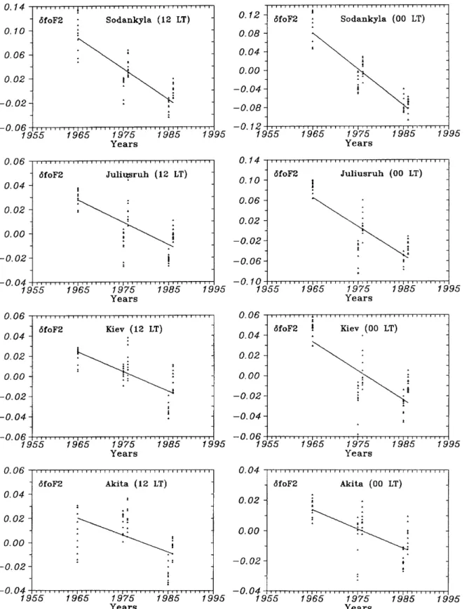
per year) of linear regression for each station, 12 and 00 SLT. Some examples of annual mean linear trends for daytime (12 LT) and nighttime (00 LT) hours are given in Fig. 1, years of solar minimum being used for the analysis. Seasonal (over 12 months) scatter in dfoF2 is shown in Fig. 1 as well. Median dfoF2 over these 12 values is found and this value is considered as the annual mean value used in further analysis.
Table 2 shows the results when years of solar maximum and minimum (Table 1) are analyzed togeth-er, while Table 3 gives the results on years of solar minimum and maximum separately. An F-test was applied to the annual mean slopes K to estimate the con®dence level. Such annual mean K values may be
considered as independent as they refer to dierent years and solar cycles. As the number of pairs N is rather small (5±14) and the scatter of individual points some-times is rather large the con®dence level may be less than 90%.
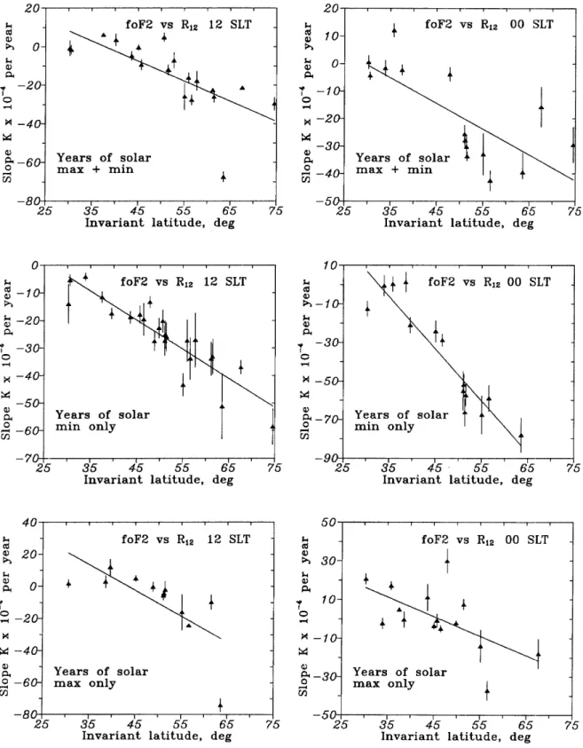
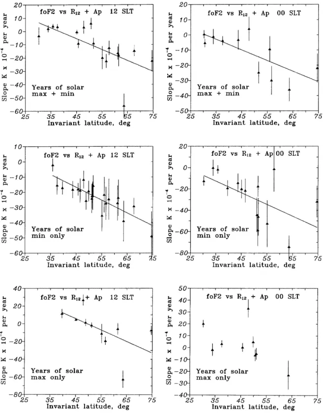
Figure 2 gives the latitudinal dependence for annual mean slopes K (model 1) for three selections of years, 12 and 00 SLT. Figure 3 shows results for the same conditions but for model 2. Only signi®cant trends from Tables 2 and 3 are included in Figs. 2 and 3. The error bars present the standard deviation over 12 monthly slopes of K. High-latitude stations with positive night-time trends (Tables 2 and 3) are not included in Figs. 2 and 3, these cases are discussed later. An analysis has shown that the invariant latitude (Table 2) usually provides better regression accuracy compared to regres-sions with geomagnetic or geodetic latitudes, so it was used in Figs. 2 and 3.
The trends revealed demonstrate a pronounced dependence on invariant latitude both for daytime and nighttime hours. Trends calculated over years of solar minimum (m) show a steeper latitudinal dependence and are more negative compared to (M + m) selection of years. In contrast, trends found over years of solar maximum (M) are more positive and are insigni®cant at the 90% con®dence level at many stations (Table 3). We
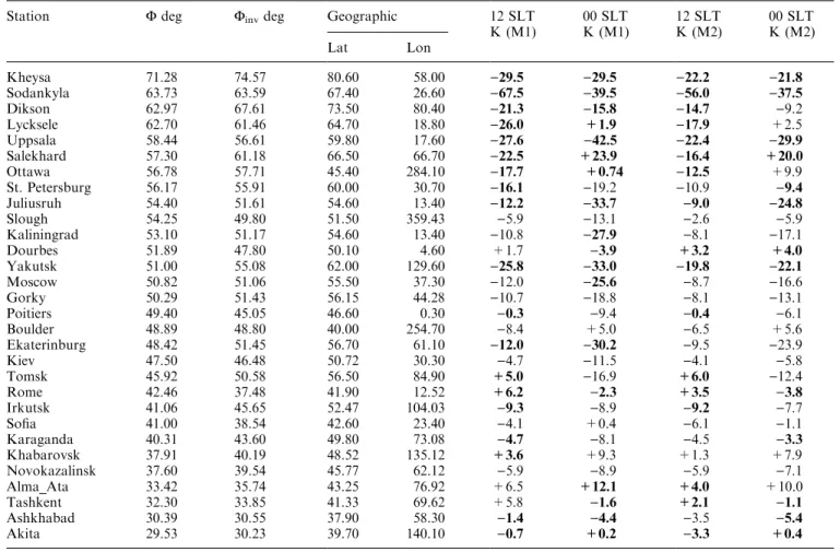
Table 2. Ionosonde stations and calculated annual mean slope K (in 10)4per year) for the period after 1965. Regressions foF2 with
R12(model 1) and with R12+ Ap (model 2) are used to make foF2
trends. Bold face ®gures show signi®cant trends with a con®dence level ³90%, normal face ®gures are trends which are not signi®cant at the 90% con®dence level
Station F deg Finvdeg Geographic 12 SLT
K (M1) 00 SLTK (M1) 12 SLTK (M2) 00 SLTK (M2) Lat Lon Kheysa 71.28 74.57 80.60 58.00 )29.5 )29.5 )22.2 )21.8 Sodankyla 63.73 63.59 67.40 26.60 )67.5 )39.5 )56.0 )37.5 Dikson 62.97 67.61 73.50 80.40 )21.3 )15.8 )14.7 )9.2 Lycksele 62.70 61.46 64.70 18.80 )26.0 +1.9 )17.9 +2.5 Uppsala 58.44 56.61 59.80 17.60 )27.6 )42.5 )22.4 )29.9 Salekhard 57.30 61.18 66.50 66.70 )22.5 +23.9 )16.4 +20.0 Ottawa 56.78 57.71 45.40 284.10 )17.7 +0.74 )12.5 +9.9 St. Petersburg 56.17 55.91 60.00 30.70 )16.1 )19.2 )10.9 )9.4 Juliusruh 54.40 51.61 54.60 13.40 )12.2 )33.7 )9.0 )24.8 Slough 54.25 49.80 51.50 359.43 )5.9 )13.1 )2.6 )5.9 Kaliningrad 53.10 51.17 54.60 13.40 )10.8 )27.9 )8.1 )17.1 Dourbes 51.89 47.80 50.10 4.60 +1.7 )3.9 +3.2 +4.0 Yakutsk 51.00 55.08 62.00 129.60 )25.8 )33.0 )19.8 )22.1 Moscow 50.82 51.06 55.50 37.30 )12.0 )25.6 )8.7 )16.6 Gorky 50.29 51.43 56.15 44.28 )10.7 )18.8 )8.1 )13.1 Poitiers 49.40 45.05 46.60 0.30 )0.3 )9.4 )0.4 )6.1 Boulder 48.89 48.80 40.00 254.70 )8.4 +5.0 )6.5 +5.6 Ekaterinburg 48.42 51.45 56.70 61.10 )12.0 )30.2 )9.5 )23.9 Kiev 47.50 46.48 50.72 30.30 )4.7 )11.5 )4.1 )5.8 Tomsk 45.92 50.58 56.50 84.90 +5.0 )16.9 +6.0 )12.4 Rome 42.46 37.48 41.90 12.52 +6.2 )2.3 +3.5 )3.8 Irkutsk 41.06 45.65 52.47 104.03 )9.3 )8.9 )9.2 )7.7 So®a 41.00 38.54 42.60 23.40 )4.1 +0.4 )6.1 )1.1 Karaganda 40.31 43.60 49.80 73.08 )4.7 )8.1 )4.5 )3.3 Khabarovsk 37.91 40.19 48.52 135.12 +3.6 +9.3 +1.3 +7.9 Novokazalinsk 37.60 39.54 45.77 62.12 )5.9 )8.9 )5.9 )7.1 Alma_Ata 33.42 35.74 43.25 76.92 +6.5 +12.1 +4.0 +10.0 Tashkent 32.30 33.85 41.33 69.62 +5.8 )1.6 +2.1 )1.1 Ashkhabad 30.39 30.55 37.90 58.30 )1.4 )4.4 )3.5 )5.4 Akita 29.53 30.23 39.70 140.10 )0.7 +0.2 )3.3 +0.4
have used stations with observations available for three solar cycles, that is with three extrema for (M) and (m) year selections. Trends for stations with two available solar extrema were not considered although they may be signi®cant according to the Fisher criterion.
Inclusion of the Ap index to the regression (model 2) makes the slopes K more positive in general and decreases the steepness of the latitudinal dependence for K. Sometimes it is even impossible to tell whether there is any latitudinal dependence for K, for instance,
Fig. 1. Some examples of annual mean foF2 trends for daytime and nighttime hours using only years of solar minimum. Triangles are individual monthly dfoF2 values
with the (M) selection of years and 00 SLT (Fig. 3, right hand, bottom).
The main results of this analysis are the following: 1. The calculated signi®cant trends are negative for the stations considered (especially for m selection of years) and demonstrate a pronounced latitudinal de-pendence with the slope K being more negative at higher invariant latitudes regardless the year selections and model used;
2. Trends calculated over the years of solar mini-mum are more negative and signi®cant on more number of stations compared to the (M) selection of years. The (m) selection of years provides a more pronounced and steeper latitudinal dependence for the slope K. Therefore, we may conclude that the inclusion of (M) years to the trend analysis in fact contaminates the initial material although not to such extent as the years during falling and rising phases of solar cycle (Danilov and Mikhailov, 1998, 1999). Therefore, the (M+m) year selection may be used for foF2 long-term trend analysis as the additional (M) years increase the statistics.
3. The revealed dependence of trends on invariant latitude clearly indicates a geomagnetic control and possible relationship with F2-layer storms (see later). An
inclusion of the Ap index in the regression in fact does not remove the geomagnetic dependence as Bremer (1992, 1998) supposed but only contaminates the ana-lyzed material increasing the scatter of points around the regression line. When model M2 is used, K depends on geomagnetic latitude as well. Therefore, further analysis is made only with model 1 as it provides purer results.
A well-pronounced dependence of foF2 trends on latitude tells us that the eect may be related to the F2-layer storms due to the long-term increase of geomag-netic activity observed after 1965 (Fig. 4, top panel). Let us analyze the results obtained from this point of view. The main processes responsible for the F2-layer storm eects are known, they are neutral composition, tem-perature, and thermospheric wind changes at middle and lower latitudes while electric ®elds and particle precipitation strongly aect the high-latitude F2-region (see ProÈlss, 1995, and references therein). The magnitude of negative storm eects increases with latitude due to a noticeable decrease in O/N2 ratio. In contrast positive
storm eects dominate at lower latitudes and they are mostly due to the increase of the equatorward thermo-spheric wind (see ProÈlss, 1995; Mikhailov et al., 1995 and references therein). Therefore, the observed depen-dence of trends on invariant latitude (Figs. 2, 3) may be just related to this F2-layer storm mechanism.
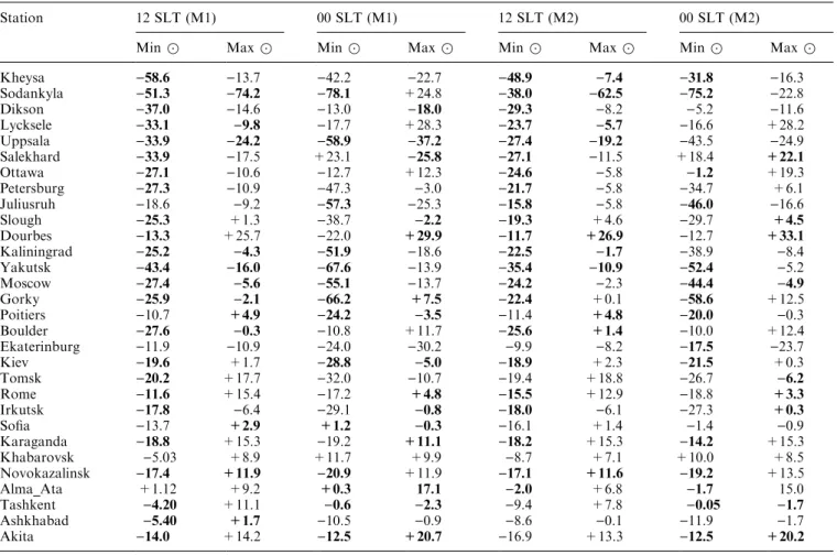
Table 3. Calculated annual mean slope K (in 10)4per year) for the
period after 1965. Regressions of foF2 with R12(model 1) and with
R12+Ap (model 2) are used to produce foF2 trends for years of
solar minimum and solar maximum. Bold face are signi®cant trends with a con®dence level ³90%, normal face are trends which are not signi®cant at the 90% con®dence level
Station 12 SLT (M1) 00 SLT (M1) 12 SLT (M2) 00 SLT (M2)
Min x Max x Min x Max x Min x Max x Min x Max x Kheysa )58.6 )13.7 )42.2 )22.7 )48.9 )7.4 )31.8 )16.3 Sodankyla )51.3 )74.2 )78.1 +24.8 )38.0 )62.5 )75.2 )22.8 Dikson )37.0 )14.6 )13.0 )18.0 )29.3 )8.2 )5.2 )11.6 Lycksele )33.1 )9.8 )17.7 +28.3 )23.7 )5.7 )16.6 +28.2 Uppsala )33.9 )24.2 )58.9 )37.2 )27.4 )19.2 )43.5 )24.9 Salekhard )33.9 )17.5 +23.1 )25.8 )27.1 )11.5 +18.4 +22.1 Ottawa )27.1 )10.6 )12.7 +12.3 )24.6 )5.8 )1.2 +19.3 Petersburg )27.3 )10.9 )47.3 )3.0 )21.7 )5.8 )34.7 +6.1 Juliusruh )18.6 )9.2 )57.3 )25.3 )15.8 )5.8 )46.0 )16.6 Slough )25.3 +1.3 )38.7 )2.2 )19.3 +4.6 )29.7 +4.5 Dourbes )13.3 +25.7 )22.0 +29.9 )11.7 +26.9 )12.7 +33.1 Kaliningrad )25.2 )4.3 )51.9 )18.6 )22.5 )1.7 )38.9 )8.4 Yakutsk )43.4 )16.0 )67.6 )13.9 )35.4 )10.9 )52.4 )5.2 Moscow )27.4 )5.6 )55.1 )13.7 )24.2 )2.3 )44.4 )4.9 Gorky )25.9 )2.1 )66.2 +7.5 )22.4 +0.1 )58.6 +12.5 Poitiers )10.7 +4.9 )24.2 )3.5 )11.4 +4.8 )20.0 )0.3 Boulder )27.6 )0.3 )10.8 +11.7 )25.6 +1.4 )10.0 +12.4 Ekaterinburg )11.9 )10.9 )24.0 )30.2 )9.9 )8.2 )17.5 )23.7 Kiev )19.6 +1.7 )28.8 )5.0 )18.9 +2.3 )21.5 +0.3 Tomsk )20.2 +17.7 )32.0 )10.7 )19.4 +18.8 )26.7 )6.2 Rome )11.6 +15.4 )17.2 +4.8 )15.5 +12.9 )18.8 +3.3 Irkutsk )17.8 )6.4 )29.1 )0.8 )18.0 )6.1 )27.3 +0.3 So®a )13.7 +2.9 +1.2 )0.3 )16.1 +1.4 )1.4 )0.9 Karaganda )18.8 +15.3 )19.2 +11.1 )18.2 +15.3 )14.2 +15.3 Khabarovsk )5.03 +8.9 +11.7 +9.9 )8.7 +7.1 +10.0 +8.5 Novokazalinsk )17.4 +11.9 )20.9 +11.9 )17.1 +11.6 )19.2 +13.5 Alma_Ata +1.12 +9.2 +0.3 17.1 )2.0 +6.8 )1.7 15.0 Tashkent )4.20 +11.1 )0.6 )2.3 )9.4 +7.8 )0.05 )1.7 Ashkhabad )5.40 +1.7 )10.5 )0.9 )8.6 )0.1 )11.9 )1.7 Akita )14.0 +14.2 )12.5 +20.7 )16.9 +13.3 )12.5 +20.2
An additional support of this concept provides the foF2 long-term variation at Slough (Fig. 4) where observations are available from the early 1930s. Long-term variations of annual mean Ap12 and dfoF2 were
analyzed for (M+m) and (m) year selections. The least
squares ®tting by the 4th (higher degree gives practi-cally the same result) degree polynomial shows the anti-phase type of dfoF2 and Ap12 long-term
varia-tions. As before error bars present the standard deviation over 12 monthly values. The periods of
Fig. 2. Daytime and nighttime annual mean slope K at stations versus invariant latitude for the period with increasing geomagnetic activity 1965±1991. Model 1 ( foF2 versus R12 regression) and three year
selections: (M+m), (m) and (M) are used in the analysis (see text).
Only stations with signi®cant trends and a con®dence level ³90% are shown. Error bars present the standard deviation of seasonal (over 12 months) scatter of the slope K
increasing geomagnetic activity (before 1945 and after 1965) are seen to correspond to negative foF2 trends while during the decreasing geomagnetic activity (1945±1965) small positive trend takes place. There is also a tendency for the trend to switch from negative to positive after 1990 in accordance with the change in geomagnetic activity (Fig. 4, top). This dependence is more pronounced for the (m) selection of years (Fig. 4,
dashes) in accordance with the discussed results. Although ®tting curves give only a qualitative picture, the extrema in Ap12 variations take place earlier or
coincide with the extrema in dfoF2 variations con®rm-ing the causal relationship between these parameters. Therefore, we may conclude that qualitatively foF2 trends at Slough station just re¯ect the long-term variation in geomagnetic activity. An increase of
geomagnetic activity results in negative foF2 trends and vice versa.
To check this conclusion diurnal variation of the trends was analyzed for the periods before and after 1965 at Slough, Moscow and Tomsk stations (Fig. 5). These three midlatitude stations are separated in longi-tude to demonstrate global character of the analyzed eect. Two (M+m) year selections over similar time intervals were chosen: 1947±1965 (18 years) and 1975± 1991 (16 years) to present the periods before and after 1965. The year 1965 is the turning-point in the long-term geomagnetic activity variation (Fig. 4. top) and if geomagnetic control of foF2 trends does exist these trends should be dierent for the two periods. Positive annual mean trends for all LT moments take place for the period prior 1965 and negative trends after 1965 for the three stations considered. Error bars give a seasonal (over 12 months) scatter in the trends. All hourly foF2 trends in Fig. 5 are signi®cant at the con®dence level ³75%. Annual mean K values were used for the F-test. Although the con®dence level is not high for some LT moments, the trends revealed demonstrate a consistent pattern of diurnal variation where individual K values seem not to be accidental.
Diurnal variations of foF2 annual mean trends at dierent invariant latitudes also clearly indicate a close
relationship of these trends with geomagnetic activity. Figure 6 gives diurnal variations of trends for: (1) a sub-auroral station, Salekhard, (2) St. Petersburg station located in the transitional (auroral/midlatitude) zone, (3) a midlatitude station, Ekaterinburg, and (4) a lower latitude station, Tashkent. The period after 1965 is considered with (M+m) selection of years. Salekhard station has strong positive trends for nighttime hours and strong negative trends during daytime.
Ekaterin-Fig. 4. Annual mean Ap12and dfoF2 at Slough long-term variations.
Two year selections (M+m) and (m) (see text) are used for the analysis. Least squares ®tting curves are a 4th degree polynomials. Error bars present the standard deviation of the seasonal (over 12 months) scatter
Fig. 5. Diurnal variation of annual mean slope K at three stations for the periods of decreasing (1947±1965) and increasing (1975±1991) geomagnetic activity. Note dierent signs of trends for the two periods. Error bars present the standard deviation of seasonal (over 12 months) scatter in the slope K
burg station demonstrates opposite behaviour with large negative nighttime trends and smaller trends during daytime hours. St. Petersburg shows mixed behaviour: the sub-auroral type for nighttime and midlatitude type during daytime hours. Low-latitude pattern of the trends is similar to the midlatitude one, but all values are more positive.
Let us consider a physical mechanism of these diurnal variations. Salekhard (Finv= 61.18°) is located
in the main ionospheric trough during nighttime hours (Muldrew, 1965; Karpachev et al., 1996) next to the equatorial boundary of the diusive precipitation zone with the increased ionization produced by soft elec-trons (see for references Besprozvannaya, 1986). The equatorial boundary of this zone is known to shift to lower latitudes by about 2° per one unity of Kp increase (e.g. Andrews and Thomas, 1969). Thus, strong posi-tive night-time trends (Fig. 6) just result from an
intensity increase of soft electron precipitation due to the overall increase in geomagnetic activity after 1965 and the shift of the precipitation zone to lower latitudes. During daytime hours the equatorial bound-ary of this zone is located far to the north at Finv = 70±80° and we have strong negative foF2 tends
resulting from the disturbed neutral composition and electric ®elds (ProÈlss, 1980; Mikhailov and Schlegel, 1998).
Midlatitude trend diurnal variations (Ekaterinburg, Fig. 6) are due to disturbed neutral composition diurnal variations. Midlatitude negative F2-layer storm eects are known to be strongest in the post-midnight-early morning LT sector and they are much weaker in the afternoon (Wrenn et al., 1987; ProÈlss, 1991, 1993, and references therein). This is due to the disturbed neutral composition with decreased O/N2ratio which is
advec-ted towards middle latitudes during night, rotates into
Fig. 6. Diurnal variation of annual mean slope K for stations located at dierent invariant latitudes (given in brackets). Note strong and opposite types of diurnal variations for sub-auroral and midlatitude
stations. Error bars present the standard deviation of seasonal (over 12 months) scatter in the slope K
the day sector being shifted back to higher latitudes by diurnal varying thermospheric circulation (Skoblin and FoÈrster, 1993; Fuller-Rowell et al., 1994; ProÈlss, 1995). This eect is clearly seen for the afternoon hours with a tendency for trends to be even positive around 1500 LT. St. Petersburg demonstrates the intermediate behav-iour. In the 03±06 LT sector this station from time to time (depending on the level of geomagnetic activity) seems to be in the soft electrons precipitation zone like Salekhard and the trends are the least negative in this LT sector. On the other hand, the increasing geomag-netic activity after 1965 results in neutral composition and temperature perturbations and strong negative trends are seen in the morning LT sector. Negative trends are strongly decreased in the afternoon LT sector similar to the midlatitude station, Ekaterinburg.
As neutral composition perturbations decreases to-wards lower latitudes (e.g. ProÈlss, 1980) the magnitude of negative trends is small even in the morning LT sector at the lower latitude station, Tashkent (Fig. 6). During daytime hours the increasing geomagnetic activity damps normal northward thermospheric circulation leading to positive F2-layer storm eects (ProÈlss, 1995; Mikhailov et al., 1995) and this results in positive foF2 trends at lower latitudes (Fig. 6). The existence of strong and latitudinal dependent diurnal variations in the magnitude of the trends is a strong argument against any manmade e.g. greenhouse origin of these trends. But such variations may be explained in terms of the F2-layer storm eects related to the geomagnetic activity as was discussed earlier.
4 Discussion
A slightly modi®ed method earlier proposed by Danilov and Mikhailov (1999) was applied to the foF2 long-term trend analysis at 30 ionosonde stations. The slope K depends on latitude (Figs. 2, 3 and Tables 2, 3) with a pronounced decrease of the trend magnitude towards lower geomagnetic (invariant) latitudes for two models used in the analysis. Therefore, the proposed method of analysis with (m) or (m+M) selection of years allows us to ®nd systematic variations in trend magnitude. Meantime the other approaches (e.g. Bremer, 1998; Upadhyay and Mahajan, 1998) result in a chaos of various signs and magnitudes of the trends on various stations.
One of the key points of the proposed method providing its success is the use of 12-month running mean foF2 rather than just monthly medians. This strongly decreases the scatter in the analyzed material helping to reveal the trends. The application of an F-test to such smoothed observations to estimate the signi®-cance of the trends may be questionable as the ®ltered data turn out to be dependent to some extent. However, it should be stressed that we use annual mean dfoF2 values belonging either to dierent solar cycles or dierent years, that is separated by 12 months. This span equals the ®ltering running interval and our values turn out to be at the opposite ends of the smoothing
interval, virtually not aecting each other. Therefore, such annual mean dfoF2 values may be considered as independent. Due to relatively small number of pairs analyzed, the con®dence level is not high (about 75%) in some cases. But this is not important as the latitudinal and diurnal variations of the trends give, as a whole, a consistent picture showing the relationship to geo-magnetic activity. On the other hand, one should keep in mind that all observed time series in geophysics and meteorology strictly speaking are never independent, nevertheless statistical methods are widely applied to such observations in practice (Panofsky and Brier, 1958). An example of the F-test application to the ionospheric trend analysis may be found in Bremer (1998). Estimating the signi®cance of the trends he used hourly F2-layer parameter observations which are known to be strongly correlated.
The sunspot number R12 usually used in empirical
ionospheric models is far from being the best (Mikhailov and Mikhailov, 1999) and in fact this index does not allow us to exclude completely the dependence on solar activity being used in foF2 versus R12regression. As the
``useful signal'' is very small in the trend analysis this imperfection of R12results in scatter in analyzed points
and various slopes K (both sign and magnitude) are obtained at various stations when all years are analyzed. The worst correlation of foF2 with R12 takes place for
the falling and rising phases of the solar cycles (the hysteresis eect), so these years were omitted from the analysis in the ®rst place (Danilov and Mikhailov, 1998, 1999). The years around solar maximum are also subjected to this uncertainty, but to a less extent and their inclusion to the trend analysis allows us, neverthe-less, to obtain a consistent pattern of trends over all stations considered. Of course, the best way for the foF2 trend analysis would be not to use any reduction on solar activity with an index like R12. Our analysis for
years of solar minimum when the solar activity reduc-tion is the minimal gives the most consistent results: all signi®cant trends are negative with well-pronounced and steep dependence of K on invariant latitude (Table 3 and Figs. 2, 3). Acceptable results are obtained with the (M+m) selection of years as well. This tells us that the contaminating eect of the (M) years inclusion is not that strong. Indeed, a pronounced dependence of K on latitude takes place for (M) selection of years as well (Figs. 2, 3). Therefore, the (M+m) year selection may be recommended for the foF2 trend analysis as was proposed earlier by (Danilov and Mikhailov, 1998, 1999). An inclusion of (M) years may be important as well for stations where the period of observation is not long enough to work with (m) years only. For instance, we used the (M+m) selection of years in Fig. 5 to increase the number of points for the period before 1965.
Although there is an obvious relationship of foF2 trends with geomagnetic activity, the monthly Ap index is not a proper indicator for the F2-layer storm eects and its inclusion to the regression (model 2), in fact, does not remove the dependence on geomagnetic activ-ity as supposed by Bremer (1998) and Jarvis et al.
(1998). Indeed, a well-pronounced dependence of K on latitude takes place for model M2 as well (Fig. 3) with the decreased trend magnitudes only. Thus, we may conclude that the inclusion of Ap indices to the regression excludes the geomagnetic eect only partly without changing, in principle, the dependence of trends on geomagnetic (invariant) latitude. Moreover, the inclusion of Ap indices to the regression (model M2) inserts additional noise to the analyzed material increas-ing the scatter of points around the regression line (see Figs. 2 and 3, left hand columns). This is not surprising as the global Ap index cannot, in principle, take into account the whole complexity of F2-layer storm eects with positive and negative phases depending on season, UT and LT of storm onset, storm magnitude etc. Thus, the Ap index inclusion cannot be recommended for the F2-layer trend analysis.
It should be stressed that our conclusions contradict those in the recent publication by Bremer (1998). He found no latitudinal eect in the trends, but revealed a separation of the stations to two longitudinal groups with positive trends in Eastern Europe and negative ones in Western Europe. We found no such longitudinal eect as most of the revealed trends are negative regardless of longitude, but there is a well-pronounced latitudinal dependence. We believe that the reason for the contradiction with the results of Bremer (1998) lies in the dierences of approach. Bremer (1998) used absolute deviations from some model and all the years available for a given station. In this case the length of the data series used is inevitably quite dierent depend-ing on the duration of the vertical sounddepend-ing observa-tions at this particular ionosonde. However, the sign of trends is dierent for the period prior to and after 1965, as follows from Fig. 5. This was the reason to separate these periods in our analysis. Further, Bremer (1998) analyzed annual trends averaging hourly and monthly values, but foF2 trends demonstrate strong diurnal variations as was shown earlier (Figs. 5, 6) and this inevitably will decrease the reliability of the trends revealed.
The proposed F2-layer storm induced mechanism for the foF2 long-term trends implies corresponding trends in hmF2. For the period with increasing geomagnetic activity and negative foF2 trends, as we have after 1965, one should expect positive hmF2 trends at middle and lower latitudes. The trends should be inverse for the period with decreasing geomagnetic activity. This fol-lows from a well-known F2-layer negative storm mech-anism related to neutral composition and temperature changes (e.g. ProÈlss, 1995). Unfortunately, hmF2 trends inferred from M(3000)F2 are not as reliable as foF2 trends, nevertheless such analysis is being done and results will be published elsewhere. It is worth mention-ing that there are indications of some long-term trends in the occurrence frequency of ionospheric storms (Sergeenko and Kuleshova, 1995; Sergeenko and Gi-vishvili, 1997; Clilverd et al., 1998). This is in line with the proposed concept on the foF2 trends mechanism.
Total cooling of the upper atmosphere due to the greenhouse eect and related negative trend in hmF2 is
discussed in some publications (e.g. Bremer, 1992; Ulich and Turunen, 1997). However, it may be shown that thermospheric temperature decrease would result in a positive trend in foF2 contrary to the observations. According to the isobaric F2-layer concept by Rishbeth and Edwards (1989, 1990) the F2-layer peak follows, in its variations, the level of constant atmospheric pressure. This is a good approximation, at least during daytime hours, when vertical plasma drifts are not strong. Electron concentration NmF2 for a steady-state day-time midlatitude F2-layer is given by the expression of Rishbeth and Barron (1960):
Nm 0:75qbm
m 3
where qm and bm are given at the F2-layer maximum.
For estimates it may be assumed that q µ [O] and b µ T2
[N2]. Then we may write using Eq (3)
D log Nm D logNOm
2mÿ 2D log T : 4
If [O] and [N2] (molecular mass m1 and m2) are
distributed in accordance with the barometric law n n0TT0exp ÿ Zh h0 dh H 8 > < > : 9 > = > ; 5
where H = kT/mg and n0and T0are the concentration
and temperature at the base height h0, the pressure and
R = [N2]/[O] at any height are related by the expression
P kT0n m2 m2ÿm1 10 nm2ÿm1m1 20 Rm2ÿm1m1 1 R : 6
It follows from Eq. (6) that the ratio R remains constant at any ®xed value of pressure P and at any temperature height pro®le provided T0, n10and n20are constant. This
is valid for any height and for hmF2 as well, so the ®rst term in Eq. (4) equals zero. Therefore, the expected temperature decrease due to the greenhouse eect should result in a positive NmF2 trend as follows from Eq. (4), thus contradicting the observed negative NmF2 trends. This dependence on temperature is due to the (O++N
2) reaction rate constant temperature
depen-dence. A steep quadratic dependence for this rate constant on T follows from the McFarland et al. (1973) laboratory measurements. Recent observations by Hierl et al. (1997) give weaker temperature depen-dence, but in any case this rate constant increases with temperature for usual ionospheric temperatures. 5 Conclusions
The main results of our analysis may be listed as follows: 1. A slightly modi®ed version of a method proposed earlier by Danilov and Mikhailov (1999) was applied to
the foF2 long-term trends analysis on 30 mid- and high-latitude ionosondes of the Northern Hemisphere. Years of solar minimum (m), maximum (M) and (M+m) were analyzed separately. Trends for 12 and 00 LT calculated over the (m) years were shown to be more negative and signi®cant at a greater number of stations compared to the (M) selection of years. The inclusion of (M) years to the trend analysis in fact contaminates the initial material although not to such extent as the years of falling and rising phases of the solar cycle (Danilov and Mikhailov, 1998, 1999). The (M+m) year selection provides an acceptable result and may be recommended for foF2 long-term trend analysis. The present analysis con®rms our previous result on the dependence of the foF2 trends on geomagnetic (invariant) latitude with strong negative trends at high and small or positive trends at lower latitudes for the period analyzed 1965± 1991.
2. The revealed dependence of the foF2 trends on invariant latitude clearly indicates the geomagnetic control and relationship with F2-layer storm mecha-nisms. An inclusion of the Ap index to the regression does not remove the geomagnetic dependence as pro-posed in some publications, but only contaminates the analyzed material without changing the result obtained in principle.
3. It is shown, for the ®rst time, that there exist periods with negative and positive foF2 trends, which correspond to the periods of long-term increasing/ decreasing geomagnetic activity. The (M+m) analysis at Slough station for instance, gives the periods with negative foF2 trends: 1934±1948, 1967±1989 and periods with positive trends: 1950±1968, and after 1989 in accordance with the smoothed variation of annual mean Ap12index used as an indicator of geomagnetic activity.
Dierent signs of the trends during the periods of increasing/decreasing geomagnetic activity take place for all LT moments at each individual station consid-ered.
4. Strong diurnal variations in the trend magnitude are revealed for stations located at dierent latitudes. Strong positive foF2 trends in the post-midnight-early morning LT sector and strong negative trends during daytime hours take place for the sub-auroral stations for the period of increasing geomagnetic activity after 1965. In contrast middle and lower latitude stations demon-strate negative trends in the early morning LT sector and small negative or positive trends during daytime hours for the same period. The existence of such diurnal variations in the foF2 trend magnitude is a strong argument against any manmade (e.g. greenhouse) origin of such trends.
5. All the morphological features revealed of the foF2 trends may be explained in the framework of contem-porary F2-region storm mechanisms. They include disturbed neutral composition, temperature and ther-mospheric winds variation (for middle and lower latitude stations) as well as soft electron precipitation for sub-auroral stations. This newly proposed geomag-netic storm concept to explain the foF2 long-term trends proceeds from a natural origin of the trends rather than
an arti®cial one related to the thermosphere cooling due to the greenhouse eect.
Acknowledgements. This work was in part supported by the Russian foundation for Fundamental Research under Grant 00-05-64189.
The Editor-in-Chief thanks two referees for their help in evaluating this paper.
References
Andrews, M. K., and J. O. Thomas, Electron density distribution above the winter pole, Nature, 221(5577), 223±227, 1969. Besprozvannaya, A. S., Planetary scale distribution of electron
concentration in the dark polar F2-region, in Ionosphere-magnetic disturbances at high latitudes, Gidrometeoizdat, L., (in Russian) 105±162, 1986.
Bremer, J., Ionospheric trends in mid-latitudes as a possible indicator of the atmospheric greenhouse eect, J. Atmos. Terr. Phys., 54, 1505±1511, 1992.
Bremer, J., Trends in the ionospheric E and F regions over Europe, Ann. Geophysicae, 16, 986±996, 1998.
Clilverd, M. A., T. D. G. Clark, E. Clake, and H. Rishbeth, Increased magnetic storm activity from 1868 to 1995, J. Atmos. Solar-Terr. Phys., 60, 1047±1056, 1998.
COST 251, Improved quality of service in ionospheric telecom-munication systems planning and operation, Final Report Ed. R. Hunbaba, p. 119, 1999.
Danilov, A. D., Long-term changes of the mesosphere and lower thermosphere temperature and composition, Adv. Space Res., 20(11), 2137±2147, 1997.
Danilov, A. D., Review of long-term trends in the upper mesosphere, thermosphere and ionosphere, Adv. Space Res., 22(6), 907±915, 1998.
Danilov, A. D., and A. V. Mikhailov, Long-term trends of the F2-layer critical frequencies: a new approach, Proceedings of the 2nd COST 251 Workshop ``Algorithms and models for COST 251 Final Product'', 30±31 March, 1998, Side, Turkey, Rutherford Appleton Laboratory, UK, 114±121, 1998.
Danilov, A. D., and A. V. Mikhailov, Spatial and seasonal variations of the foF2 long-term trends, Ann. Geophysicae, 17, 1239±1243, 1999.
Fuller-Rowell, T. J., M. V. Codrescu, R. J. Moett, and S. Quegan, Response of the and ionosphere to geomagnetic storm, J. Geo-phys. Res., 99, 3893±3914, 1994.
Givishvili, G. V., and L. N. Leshchenko, Possible proofs of presence of technogenic impact on the midlatitude ionosphere, Doklady RAN, 334(2), (in Russian) 213±214, 1994.
Givishvili, G. V., and L. N. Leshchenko, Dynamics of the climatic trends in the midlatitude ionospheric E region, Geomag. Aeronom., 35(3), (in Russian) 166±173, 1995.
Givishvili, G. V., and L. N. Leshchenko, Regional dierences in long-term variations of the aeronomic parameters in the midlatitude upper atmosphere, Doklady RAN, 346(6), (in Russian) 808±811, 1996.
Givishvili, G. V., and L. N. Leshchenko, Long-term variation in the critical frequency of the midlatitude E-layer, Proceedings of the International Workshop ``Cooling and Sinking of the Middle and Upper Atmosphere, Moscow, July 6±10, 1998'', p. 30, 1998. Givishvili, G. V., L. N. Leshchenko, O. P. Shmeleva, and T. G.
Ivanidze, Climatic trends of the mid-latitude upper atmosphere and ionosphere, J. Atmos. Terr. Phys., 57(8), 871±874, 1995. Hierl, P. M., I. Dotan, J. V. Seeley, J. M. Van Doran, R. A. Morris,
and A. A. Viggiano, Rate coecients for the reactions of O+
with N2 and O2 as a function of temperature (300±188 K),
J. Chem. Phys., 106(9), 3540±3544, 1997.
Jarvis, M. J., B. Jenkins, and G. A. Rodgers, Southern Hemisphere observations of a long-term decrease in F region altitude and thermospheric wind providing possible evidence for global
thermospheric cooling, J. Geophys. Res., 103, 20 774±20 787, 1998.
Karpachev, A. T., M. G. Deminov, and V. V. Afonin, Model of the mid-latitude ionospheric trough on the base of Cosmos-900 and Intercosmos-19 satellites data, Adv. Space Res., 18(6), 221±230, 1996.
McFarland, M., D. L. Albritton, F. C. Fehsenfeld, E. E. Ferguson, and A. L. Schmeltekopf, Flow-drift technique for ion mobility and ion-molecular reaction rate coecient measurements. II. Positive ion reactions of N+, O+, and N
2 with O2and O+with
N2from thermal to 2 eV, J. Chem. Phys., 59, 6620±6628, 1973.
Mikhailov, A. V., Ionospheric index MF2n for monthly median foF2 modeling and long-term prediction over European area, Phys. Chem. Earth (C), 24, 329±332, 1999.
Mikhailov, A. V., and V. V. Mikhailov, A new ionospheric index MF2, Adv. Space Res., 15(2), 93±98, 1995.
Mikhailov, A. V. and V. V. Mikhailov, Indices for monthly median foF2 and M(3000)F2 modeling and long-term prediction: ionospheric index MF2, Inter. J. Geomagn. Aeronom., 1, 141± 151, 1999.
Mikhailov, A. V., and K. Schlegel, Physical mechanism of strong negative storm eects in the daytime ionospheric F2 region observed with EISCAT, Ann. Geophysicae, 16, 602±608, 1998. Mikhailov, A. V., M. G. Skoblin, and M. FoÈrster, Daytime F2-layer
positive storm eect at middle and lower latitudes, Ann. Geophysicae, 13, 532±540, 1995.
Mikhailov, A. V., V. V. Mikhailov, and M. G. Skoblin, Monthly median foF2 and M(3000)F2 ionospheric model over Europe, Ann. Geo®s, 39, 791±805, 1996.
Muldrew, D. B., F-layer ionization trough deduced from Alouette data, J. Geophys. Res., 70, 2635±2650, 1965.
Panofsky, H. A., and G. W. Brier, Some applications of statistics to meteorology, Pennsylvania State University, 1958.
Pollard, J. H., A handbook of numerical and statistical techniques, Cambridge University Press, 1977.
ProÈlss, G. W., Magnetic storm associated perturbations of the upper atmosphere: recent results obtained by satellite-borne gas analyzers, Rev. Geophys. Space Phys., 18, 183±202, 1980. ProÈlss, G. W., Solar wind energy dissipation in the upper
atmosphere, Adv. Space Res., 3(1), 55±66, 1983.
ProÈlss, G. W., Thermosphere-Ionosphere coupling during dis-turbed conditions, J. Geomagn. Geoelectr., 43 (Supp), 537±549, 1991.
ProÈlss, G. W., On explaining the local time variation of ionospheric storm eects, Ann. Geophysicae, 11, 1±9, 1993.
ProÈlss, G. W., Ionospheric F region storms, in Handbook of atmospheric electrodynamics, 2, Ed. H. Volland, 195±248, CRC Press, Boca Raton, Fla., 1995.
Rishbeth, H., A greenhouse eect in the ionosphere?, Planet. Space Sci., 38, 945±948, 1990.
Rishbeth, H., Long-term changes in the ionosphere, Adv. Space Res., 20, (11)2149±(11)2155, 1997.
Rishbeth, H., and D. W. Barron, Equilibrium electron distributions in the ionospheric F2-layer, J. Atmos. Terr. Phys., 18, 234±252, 1960.
Rishbeth, H., and R. Edwards, The isobaric F2 layer, J. Atmos. Terr. Phys., 51, 321±338, 1989.
Rishbeth, H., and R. Edwards, Modeling the F2 layer peak height in terms of atmospheric pressure, Radio Sci., 25, 757±769, 1990. Rishbeth, H., and R. G. Roble, Cooling of the upper atmosphere
by enhanced greenhouse gases ± modelling of thermospheric and ionospheric eects, Planet. Space Sci., 40, 1011±1026, 1992.
Sergeenko, N. P., and V. P. Kuleshova, Long-term trends of the F2 layer ionospheric disturbances, Geomagn. Aeronom., 35(5), (in Russian) 128±130, 1995.
Sergeenko, N. P., and G. V. Givishvili, On the problem of the long-term trends in the ionospheric disturbances characteristics, Geomagn. Aeronom., 37(2), (in Russian) 109±113, 1997. Skoblin, M. G., and M. FoÈrster, An alternative explanation of
ionization depletion in the winter night-time storm perturbed F2 layer, Ann. Geophysicae, 11, 1026±1032, 1993.
Ulich, T., and E. Turunen, Evidence for long-term cooling of the upper atmosphere in ionospheric data, Geophys. Res. Lett., 24, 1103±1106, 1997.
Upadhyay, H. O., and K. K. Mahajan, Atmospheric greenhouse eect and ionospheric trends, Geophys. Res. Lett., 25, 3375± 3378, 1998.
Wrenn, G. L., A. S. Rodger, and H. Rishbeth, Geomagnetic storms in the Antarctic F-region. I. Diurnal and seasonal patterns for main phase eects, J. Atmos. Terr. Phys., 49, 901±913, 1987.