HAL Id: hal-01475674
https://hal.archives-ouvertes.fr/hal-01475674
Submitted on 24 Feb 2017
HAL is a multi-disciplinary open access
archive for the deposit and dissemination of
sci-entific research documents, whether they are
pub-lished or not. The documents may come from
teaching and research institutions in France or
abroad, or from public or private research centers.
L’archive ouverte pluridisciplinaire HAL, est
destinée au dépôt et à la diffusion de documents
scientifiques de niveau recherche, publiés ou non,
émanant des établissements d’enseignement et de
recherche français ou étrangers, des laboratoires
publics ou privés.
A geostatistical approach to the simulation of stacked
channels
Guillaume Rongier, Pauline Collon, Philippe Renard
To cite this version:
Guillaume Rongier, Pauline Collon, Philippe Renard.
A geostatistical approach to the
simu-lation of stacked channels.
Marine and Petroleum Geology, Elsevier, 2017, 82, pp.318 - 335.
�10.1016/j.marpetgeo.2017.01.027�. �hal-01475674�
Marine and Petroleum Geology, 82: 318–335, 2017
10.1016/j.marpetgeo.2017.01.027
A geostatistical approach to the simulation
of stacked channels
Guillaume Rongier
1,2, Pauline Collon
1, and Philippe Renard
2 1GeoRessources (UMR 7359, Université de Lorraine/ CNRS / CREGU), Vandœuvre-lès-Nancy, F-54518 France 2Centre d’Hydrogéologie et de Géothermie, Université de Neuchâtel, 11 rue Emile-Argand, 2000 Neuchâtel, SwitzerlandAbstract Turbiditic channels evolve continuously in relation to erosion-deposition events. They are often gathered into complexes and display various stacking patterns. These patterns have a direct impact on the connectivity of sand-rich deposits. Being able to reproduce them in stochastic simulations is thus of significant importance. We propose a geometrical and descriptive approach to stochastically control the channel stacking patterns. This approach relies on the simulation of an initial channel using a Lindenmayer system. This system migrates proportionally to a migration factor through either a forward or a backward migra-tion process. The migramigra-tion factor is simulated using a sequential Gaussian simulamigra-tion or a multiple-point simulation. Avulsions are performed using a Lindenmayer system, similarly to the initial channel simulation. This method makes it possible to control the connectivity between the channels by adjusting the geometry of the migrating areas. It furnishes encour-aging results with both forward and backward migration processes, even if some aspects such as data conditioning still need to be explored.
Keywords
Sedimentary system Channel
Migration
Stochastic simulation
Sequential Gaussian simulation Multiple-point simulation
1 Introduction
Heterogenities within turbiditic channel deposits can have a dramatic impact on fluid flow and reservoir production[e.g., Gainski et al.,2010]. Mud-rich deposits such as margin drapes or slumps can obstruct fluid circulation and compartmentalize the reservoir depending on the stacking pattern[Labourdette et al.,2006], i.e., how channels position themselves in relation to each others. Significant changes in the stacking pattern can be observed even over short distances[Mayall and O’Byrne, 2002]. This represents a major source of uncertainty regarding the connectivity, and modeling the stacking can help to assess this uncertainty.
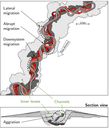
This stacking results from two main processes: channel mi-gration and avulsion. Mimi-gration occurs either through the gradual erosion and accretion of sediments along the chan-nel margins, called continuous migration[e.g.,Abreu et al., 2003, Arnott,2007,Nakajima et al.,2009], or through the incision and filling of a new channel, sometimes with a signifi-cant distance between the channels, called discrete or abrupt migration[e.g.,Abreu et al.,2003,Deptuck et al.,2003,Maier et al.,2012]. Four patterns stand out (figure1):
• A lateral channel bend migration or swing, which shifts the bend laterally and increases the channel sinuosity [Peakall et al.,2000,Posamentier,2003].
• A downsystem channel bend migration or sweep, which shifts the bend downward[Peakall et al.,2000, Posa-mentier,2003].
• A channel bend retro-migration, which decreases the channel sinuosity[Nakajima et al.,2009].
• A vertical channel migration or aggradation, which
shifts the channel upward[Peakall et al.,2000]. Avulsion occurs when the density currents exceed the channel capacity to contain them: the flow leaves the channel and forms a new course.
Simulating migration and avulsion is a central research sub-ject to better model the channel stacking. In fluvial systems, the most widespread methods are two-dimensional physical simu-lations[Lopez,2003,Pyrcz et al.,2009]. They link the migra-tion to the asymmetry in the flow field induced by the channel curvature, which is responsible for bank erosion[Ikeda et al., 1981]. These two-dimensional physical methods have been applied[McHargue et al., 2011] and adapted [Imran et al., 1999] to turbiditic environments. But the physical processes behind submarine channels remain controversial. The main controversy concerns the rotation direction of the secondary flow and its controlling factors[e.g.,Corney et al.,2006, Im-ran et al.,2008,Corney et al.,2008], which constrain channel migration. Dorrell et al.[2013] argue that two-dimensional physical models are not accurate enough to capture the full three-dimensional structure of the flow field. This lack of ac-curacy was also pointed out in fluvial settings, especially with simplified physical models[Camporeale et al.,2007]. More complex two-dimensional models or three-dimensional models call for more parameters and a bigger computational effort, and their validity remains questioned[e.g.,Sumner et al.,2014]. Thus, their convenience in a stochastic framework is doubtful. Another approach proposes to only reproduce some strati-graphic rules, for instance mimicking the migration without actually simulating the physical processes[Pyrcz et al.,2015]. Viseur[2001] andRuiu et al.[2015] defined migration vectors from a weighted linear combination of vectors for lateral mi-gration, downsystem mimi-gration, and bend rotation.Teles et al. [1998],Labourdette[2008] andLabourdette and Bez[2010]
Map view Lateral migration Abrupt migration Downsystem migration Section view Aggration
Inner levees Channels
Figure 1 Example of channel migration patterns interpreted on seis-mic data from the Benin-major channel-belt, near the Niger Delta (modified fromDeptuck et al.[2003]).
went one step further by defining empirical laws controlling the spatial structure of the migration from modern channels or channels interpreted on seismic data. All such methods derive from object-based approaches, which simulate a channel ob-ject. On the other hand, cell-based approaches[e.g.,Deutsch and Journel,1992,Mariethoz et al.,2010] paint the channels inside a grid based on a prior model. This prior model describes spatial structures and their relationships. Such methods can simulate almost any structure with few parameters. However, they have difficulties reproducing continuous channelized bod-ies and are not designed to model channel migration. Here we propose a different approach to channel migration, combining object- and pixel-based approaches as done with other geolog-ical structures[e.g.,Caumon et al.,2007,Zhang et al.,2009, Rongier et al.,2014].
The proposed channel migration method uses a geostatis-tical simulation to reproduce the spatial structure resulting from the physical processes rather than modeling the physical processes themselves. We stochastically simulate the spatial evolution of a channel from one stage to the next using either a sequential Gaussian simulation (SGS) or a multiple-point simulation (MPS) method (section2). Such a descriptive ap-proach avoids the use of physical models that can be difficult to parameterize. After describing its capabilities (section3), the method is applied to a synthetic case of confined turbiditic channels (section4). This case includes a comparison of the connectivity from migrated channels and from randomly im-planted channels. Finally, we discuss those results along with some perspectives for the method (section5).
2 Stochastic simulation of channel
evolu-tion
We divide channel migration into two elements:
• The horizontal component (hereafter referred to as mi-gration), which includes the lateral, downsystem, and retro-migrations.
• The vertical component (hereafter referred to as aggra-dation), which includes the vertical migration.
[Labourdette,2008] proposed to initiate the process from the last channel of a system, so from the youngest channel, and migrate backward. Indeed, this last channel is often observable on seismic data due to its argileous fill. Then the migration divides in two processes:
• A forward migration, which is the normal or classical migration. It starts from the oldest channel in geological time, which migrates to obtain the youngest channel. • A backward migration, which is a reverse migration.
It starts from the youngest channel in geological time, which migrates to obtain the oldest channel.
We propose a process to handle both forward and backward channel migrations.
2.1 Channel initiation
The simulation calls for an already existing channel to initiate the evolution process. This initial channel can be interpreted from seismic data with a high enough resolution. Otherwise, it must be simulated. Here we use a formal grammar, the Lindenmayer system (L-system)[Lindenmayer,1968], for this simulation.
The L-system rewrites an initial string using rules, which replace a set of letters by another one. The resulting string is then interpreted into an object.Rongier[2016] defined some rules in a framework able to stochastically simulate a chan-nel from a L-system. These rules tie chanchan-nel bends together, controlling the bend morphology and the orientation change between each bend. It results in a channel centerline, i.e., a set of locations through which the channel passes. Non-Uniform Rational B-Spline (NURBS) surfaces dress the L-system to ob-tain the final channel shape[Ruiu et al.,2015].
This method simulates various meandering patterns, from straight to highly sinuous channels. It is suitable for both for-ward migration, which classically requires starting with a quite straight channel, and backward migration, which requires an initial channel with a high sinuosity.
2.2 Channel migration
Channel migration is deeply linked to the channel curvature. Other elements have to be considered, such as soil properties or flow fluctuations. However, the physical processes behind bend evolution are complex and still not completely under-stood. Moreover, they differ from turbiditic to fluvial environ-ments. This is why we propose to rely on a more descriptive approach based on geostatistics.
A B ~ va= εazˆ ~ vm= εmnˆ A B Scale: ×3 ˆ n ˆ s ˆ z ~ vm= εmnˆ Initial channel Migrated channel Centerline node Distance increase Distance decrease
Figure 2 Migration principle: the centerline nodes are moved along the vectorsv~aandv~m.v~ais the aggradation component along the verti-cal direction symbolized by the normalized vector ˆz. The aggradation factor"adetermines the vertical displacement. v~mis the migration component along the normal direction to the centerline symbolized by the normalized vector ˆn. The migration factor"mdetermines the hori-zontal displacement. ˆsis the normalized vector along the streamwise direction.
2.2.1 General principle
In physical approaches, a migration factor is computed along the nodes of a channel centerline based on fluid flow equa-tions. Then the nodes are moved based on that factor along the normal to the centerline.
We rely on a similar approach based on moving the nodes along the normal to the centerline to migrate a channel (fig-ure2). Here the Euclidean distance d of displacement for a node is the length of a displacement vector~v:
d= k~vk (1)
The displacement vector divides into two components (fig-ure2):
• A vertical component for the aggradation. Aggradation is simply done by shifting the new channel vertically by an aggradation factor"a, which is the same for all the channel nodes.
• A horizontal component defined by a migration factor "mcomputed using a stochastic simulation method. The stochastic simulation of the migration factor is done either with sequential Gaussian simulation (SGS) or multiple-point
simulation (MPS). In both cases, the curvature becomes a sec-ondary variable that influences the structuring of the migration factor. We detail some numerical aspects valid for both the SGS and MPS in the supplementary materials concerning:
• Curvature computation.
• Regridding to preserve a constant distance between the centerline nodes after migration (figure2).
• Smoothing to eliminate undesired small-scale fluctua-tions of the migration factor, which can have a signifi-cant impact after some migration steps.
2.2.2 Migration through sequential Gaussian simulation The SGS simulates a migration factor value for each node of the centerline in a sequential way[e.g.,Deutsch and Journel, 1992]. Here we use an intrinsic collocated cokriging [Babak and Deutsch,2009] to introduce the curvature as secondary variable:
1. A random path is defined to visit all the centerline nodes. 2. At a given node:
a) If some nodes in a given neighborhood already have a value:
i. A kriging system determines the Gaussian complementary cumulative distribution func-tion (ccdf) using the data, i.e., the nodes with a value given in input and the previously sim-ulated nodes within the neighborhood. ii. A simulated value for the given node is drawn
within the ccdf.
b) Otherwise, the simulated value is drawn from an input distribution of migration factor.
3. Return to step 2 until all the nodes of the path have been visited.
The SGS requires the migration factor to be a Gaussian variable. If not, a normal score transform of the input distribution and of the data is introduced before step 1. A back transform is done at the end of the simulation process.
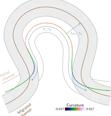
This simulation of the migration calls at least for four pa-rameters (figure3, see the supplementary materials for more details):
• Two distributions, one for the aggradation factor"aand one for the migration factor"m. They control the dis-tance between two successive channels.
• A variogram range r. It controls the extension of the migrating area along a bend. The other variogram pa-rameters get default values.
• A curvature weightγc. It represents the correlation be-tween the primary variable, i.e., the migration factor, and the secondary variable, i.e., the curvature. When this weight is positive, the channel tends to migrate, when it is negative, the channel tends to retro-migrate. Thus, simply by changing the curvature weight symbol the same workflow achieves both forward and backward migration processes.
εm, γc r, γc Initial channel Migrated channel Curvature -0.017 0.017
Figure 3 Main parameters used for horizontal bend migration with SGS. "mis the migration factor, r the variogram range andγc the curvature weight. The later perturbs the two other parameters by fitting more or less the migration spatial structure to the curvature spatial structure.
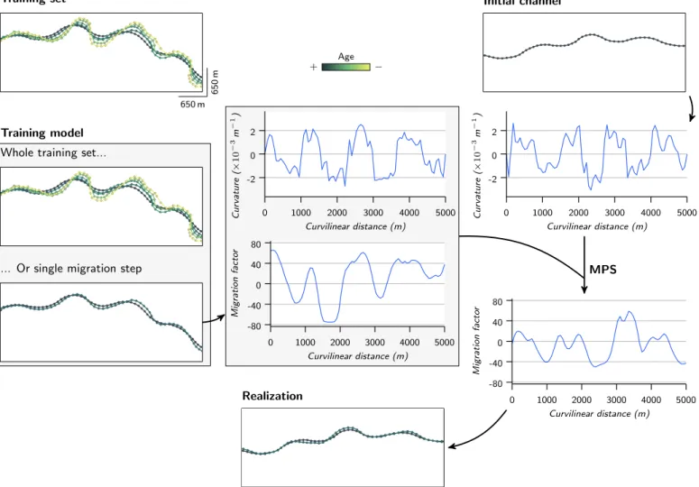
2.2.3 Migration through multiple-point simulation Simulation methods such as the SGS rely on a histogram and a variogram inferred from the data. Thus, they only catch the one- and two-point statistics and miss all the higher-order statistics. But higher-order statistics are difficult if not impos-sible to infer from data. Multiple-point simulation[Guardiano and Srivastava,1993] attempts to overcome such limitation by relying on an external representation of the structures of interest, the training image. Here the training image is a set of migrating channels, with the aggradation factor, migration fac-tor and curvature values all known. Using MPS instead of SGS could lead to more realistic migrations by using real channels as training set.
The whole training set is not necessarily used to simulate the migration of a channel. The process relies on a training model, which can be (figure4):
• The entire training set. In this case, each simulated migration step is influenced by all the migration steps within the training set.
• A single migration step within the training set:
– Drawn randomly among all the migration steps of
the training set.
– That follows the migration order of the training
set. In that case, each simulated migration step corresponds to a particular migration step within the training set. With that option, the number of migration steps in the training set limits the number of simulated migration steps.
The aggradation values are randomly drawn from the train-ing set and attributed to all the nodes of the channel to migrate.
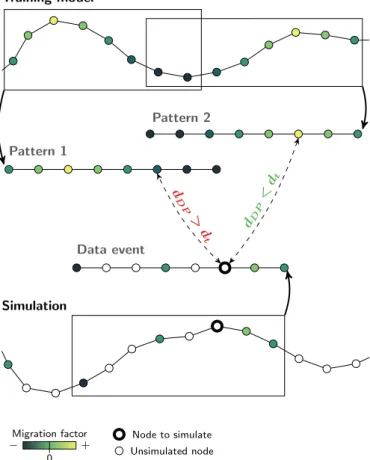
The migration factor is simulated using the Direct Sampling method (DS)[Mariethoz et al.,2010]:
1. A random path is defined to visit all the centerline nodes. 2. At a given node (figure5):
a) The n closest nodes with already a value form two data events Nx, one for the migration factor and one for the curvature.
b) Those data events are searched within the training model:
i. A position is randomly chosen and the train-ing model is then scanned linearly.
ii. At a given node:
A. Two distances dD,P are computed be-tween the current pattern Ny and the data event Nx, one for the migration fac-tor and one for the curvature:
dD,P(Nx, Ny) = 1 n n X i=1 Z(xi) − Z(yi) max
y∈T M(Z(y)) − miny∈T M(Z(y)) (2) with dD,P∈ [0, 1], n the number of nodes in the data event, Z the compared prop-erty, x a node in the data event, y a node in the training set pattern and T M is the training model.
B. If the distances are both the lowest en-countered, the value of the central node associated to the pattern is saved. C. If the distances are both lower than given
thresholds, the scan stops.
a) The saved value becomes the simulated value for this node.
3. Return to step 2 until all the nodes of the path have been visited.
This method has the advantage of easily handling continuous properties and secondary data, here the curvature. The cur-vature ensures the link between the spatial variations of the migration factor in the training model and in the simulation.
Besides the training model, this simulation of the migration calls for the classical DS parameters (see the supplementary materials for more details):
• The maximal number of nodes in a data event. • The maximal portion of the training model to scan. • A threshold for the migration factor.
• A threshold for the curvature.
2.3 Neck cut-off determination
As the channel sinuosity increases, the two extremities of a bend come closer one to the other until the flow bypasses the bend. This is a neck cut-off, leading to the abandonment of the bypassed bend.
As done in physical simulations[e.g.,Howard,1992, Cam-poreale et al.,2005,Schwenk et al.,2015], neck cut-offs are simply identified when two non-successive nodes of the center-line are closer than a given threshold. The lowest threshold is
Training set
Whole training set...
... Or single migration step Training model -2 0 2 0 1000 2000 3000 4000 5000 Curvilinear distance (m) Curvature (× 10 − 3m − 1) -80 -40 0 40 80 0 1000 2000 3000 4000 5000 Curvilinear distance (m) Migration facto r Initial channel -2 0 2 0 1000 2000 3000 4000 5000 Curvilinear distance (m) Curvature (× 10 − 3m − 1) -80 -40 0 40 80 0 1000 2000 3000 4000 5000 Curvilinear distance (m) Migration facto r Realization MPS Age + − 650 m 650 m
Figure 4 Framework for the simulation of the migration factor"mwith MPS.
the channel width, as the margins of the bend come in contact. However, this threshold is quite restrictive and not so realistic [Camporeale et al., 2005]. Here the threshold is set to 1.2 times the maximal channel width.
The search for cut-off starts upstream and continues to the most downstream part of the channel. The distance between a given node and another non-successive node of the centerline is compared with the threshold. When the distance is lower, these two nodes and all the nodes in-between are suppressed. The cutting path is then symbolized by two nodes. A new node is added along that path[Schwenk et al.,2015], using a cubic spline interpolation. This method of neck cut-off determination is simple but rather time-consuming. More efficient methods exist to reduce the computation time[e.g.,Camporeale et al., 2005,Schwenk et al.,2015].
For now only the forward migration process handles the for-mation of neck cut-offs. Indeed, the cut-offs appear naturally as the sinuosity increases. In the backward process, the sinu-osity decreases: introducing neck cut-offs calls for a different method, which is a perspective of this work.
2.4 Avulsion
Avulsion is a key event widely observed in both fluvial and turbiditic systems. When an avulsion occurs, the channel is abruptly abandoned at a given location (figure6). Upstream, the flow remains in the old channel, whereas downstream a new channel is formed. However, its triggering conditions
remain poorly understood due to the complexity of this process. Avulsion is often statistically handled in simulation methods: a probability of avulsion controls the development of a new channel. This process can be influenced by the curvature, as a high curvature tends to favor an avulsion.
The approach for global avulsion is similar to that defined byPyrcz et al.[2009]. The avulsion starts by computing the sum of the curvatures at each channel section. A threshold is randomly drawn between zero and the sum of curvatures. The channel is then scanned from its most upstream part to the downstream part. At each centerline node, the curvature is subtracted from the threshold. A section initiates an avulsion or not depending on two factors:
• An input probability of avulsion.
• The random curvature threshold, which should be lower than the section curvature to trigger an avulsion. Thus, the avulsion initiation at a given section is a probabilistic choice influenced by the curvature at the section location.
Then, the upstream part of the channel is isolated. It be-comes the initial string to simulate the new post-avulsion chan-nel with a L-system (figure6). This channel is based on the same parameters than the initial channel, but different parame-ter values may be used. A repulsion constraint[Rongier,2016] with the pre-avulsion channel can be set to avoid intersections between the two channels.
Training model Simulation Data event Pattern 1 Pattern 2 d D P > d t dD P < dt Migration factor 0 − + Node to simulate Unsimulated node
Figure 5 DS simulation principle: the neighboring configuration around the node to simulate, the data event, is sought within the similar configurations in the training model, the patterns. Here the neighboring configurations contains the four nodes with a known value that are the closest to the node to simulate. When the distance DDPbetween the data event and a pattern is lower than a given thresh-old dt, the process stops and the node to simulate gets the value at the same location within the pattern.
3 Applications
The method was implemented in C++ in the Gocad plug-in ConnectO. The channel envelopes based on NURBS were im-plemented by Jérémy Ruiu in the Gocad plug-in GoNURBS [Ruiu et al.,2015].
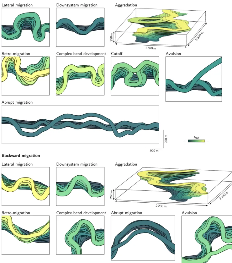
The method was used to simulate two realizations: one fol-lowing a forward migration process and one folfol-lowing a back-ward migration process (figure7). Both processes are able to reproduce various migration patterns, from lateral to down-system migration, and even areas of retro-migration (figure 8). Some bends also evolve to complex bends constituted by several bends: this leads to the formation of new meanders. These synthetic cases have been developed without any condi-tioning data. The range is chosen similar to the bend length. The other variogram parameters are those predefined (see the supplementary materials). The curvature weight is kept high, giving a dominant lateral migration. The forward process could keep migrating over more steps, with neck cut-offs keeping the channels within a restrained area. The backward process does not migrate much after a few steps, when the channel starts to miss significant bends. An avulsion and sometimes an abrupt migration can re-establish some migration.
Abrupt migrations are handled by introducing a second set of migration parameters. The channel centerline is scanned upstream to downstream. A probability of abrupt migration
Current channel Avulsed channel Upstream Downstream Avulsion location Preserved part (axiom) Abandoned part New channel path (L-system simulation)
Figure 6 Principle of global avulsion based on L-system.
defines if an abrupt migration occurs. The appearance of an abrupt migration is also weighted by the channel curvature. When an abrupt migration occurs, an abrupt migration length is drawn from an input distribution. All the nodes along the drawn length migrate following the second set of migration parameters. Such abrupt migration process can introduce a spatial discontinuity from the previous channel (figure8).
Avulsion momentarily stops the migration process, which restarts from the new channel. The continuity between the upstream part to the avulsion location and the newly simulated channel is finely preserved (figure8). The use of the curvature to weight the abrupt migration and avulsion process tends to decrease their emergence in the backward process. This is due to the sinuosity decrease induced by such process. In this case, higher probabilities are used.
Neck cut-offs naturally appear during the forward process as the sinuosity increases (figure8, forward migration). The proposed backward process is unable to generate cut-offs. As the migration advances, the channel just gets straighter. It does not evolve to a complete straight line, but continuing the process does not lead to an increase of the sinuosity: the channel remains in a steady-state.
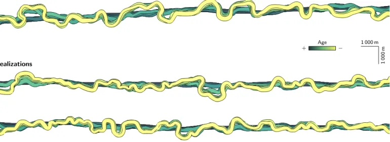
To test the method with MPS, a training set was simulated with a SGS-based process (figure9). This training set has 9
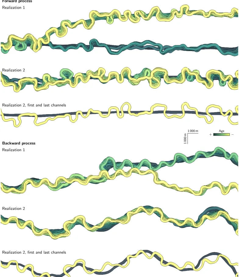
Forward process Realization 1
Realization 2
Realization 2, first and last channels
Backward process Realization 1
Realization 2
Realization 2, first and last channels
1 000 m 1 000 m Age + −
Figure 7 Examples of realizations for both the forward and backward SGS migration processes SGS initiated by channels simulated with a L-system. The input parameters are given in the supplementary materials.
Forward migration
Lateral migration Downsystem migration Aggradation
2510 m
1 660 m
250
m
Retro-migration Complex bend development Cutoff Avulsion
Abrupt migration 900 m 900 m Age + − Backward migration
Lateral migration Downsystem migration Aggradation
3 240 m
2 230 m
260
m
Retro-migration Complex bend development Abrupt migration Avulsion
Figure 8 Enlargements on some areas of the channels on figure7illustrating different aspects of channel evolution reproduced by forward and backward migration simulations.
Training set Realizations 1 000 m 1 000 m Age + −
Figure 9 Application of a forward migration process based on MPS to two channels generated with L-system. The input parameters are given in the supplementary materials.
migrating steps. Lateral migration dominates the system, and several abrupt migrations perturb the channel stacking. Each migration step simulates the migration factor from the cor-responding step in the training set, and not from the entire training set. The parameters for the MPS favor quality over speed, with the two thresholds at 0.01 and maximal scanned fraction of the training model of 0.75. But the simulated migra-tion factors are noisy, because the process can not always find a pattern that meets the thresholds. We added two smoothing iterations (see the supplementary materials) at the end of each migration step to limit the noise.
In the end, the lateral migration is still dominant in the sim-ulations. Abrupt migrations are also reproduced by the simula-tion process. But they tend to be less frequent. They also tend to be smaller, both in length and in migration factor, than in the training set. This comes from both the inability to find the right pattern in the training set and from the smoothing.
4 Analysis of the channel stacking impact
on the static connectivity
This section aims at highlighting the impact of the migration process on the simulated channel connectivity. To do so, we rely on a synthetic case study including realizations with dif-ferent stacking patterns.
4.1 Case study
The case study is inspired by turbiditic systems and their nested channelized bodies[e.g.,Abreu et al.,2003,Mayall et al.,2006, Janocko et al.,2013]. In such settings, channels migrate within and gradually fill a master channel – a large incision that con-fines the channels:
• Lateral migration dominates the first phase of the filling. The channels migrate within the whole master channel width, with a low aggradation and some abrupt lateral migrations. Sand-rich channel deposits occupy the en-tire bottom of the master channel.
• Aggradation dominates the second phase of the filling. The lateral migration is less significant, and no abrupt migration arises. Sand-rich deposits occupy a limited area within the top of the master channel. The rest of the master channel is filled with inter-channel deposits, in particular inner levees whose development induces the limited lateral migration.
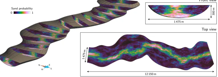
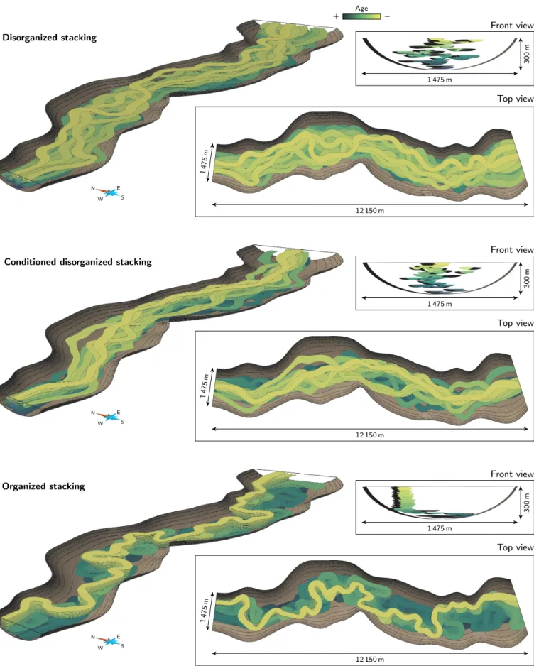
A hexahedral grid aligned along its margins represents the mas-ter channel (figure10). Three sets of 100 realizations are sim-ulated within this grid, with each realization containing 40 channels (see the supplementary materials for the input pa-rameters).
The first two sets rely on a traditional object-based proce-dure: the channels are randomly placed inside the grid. Here, each channel is simulated using a L-system, similarly to the ini-tial channel for the migration. L-systems condition data thanks to attractive and repulsive constraints[Rongier,2016]: in the proposed application, the master channel margins repulse the channels to keep them confined. The first set (figure11, a) is limited to this setting: its channels are free to occupy the whole grid without any constraint on their relative location. These channels display a disorganized stacking. The second set (figure11, b) further uses the L-system ability to condition data to reproduce the two-phase evolution of the channels. The random channel placement and the channel development are both influenced by a sand probability cube that defines the sand-rich deposit distribution inside the grid (figure10). It in-fluences the relative positions of the channels without directly controlling the channel relationships. These channels display a conditioned disorganized stacking.
The last set (figure11, c) also attempts to reproduce the two-phase channel evolution, but without using the probabil-ity cube. Instead, it directly simulates this evolution with a forward SGS-based migration. The first 27 migration steps simulate a high lateral migration, some abrupt migrations and little aggradation. This first phase is initiated with a channel simulated with a L-system, whose initial position is randomly drawn at a fixed vertical coordinate along the bottom of the grid. The next 12 steps simulate a small lateral migration with a significant aggradation. This second phase is initiated with
N W E S Top view 1475 m 12 150 m Front view 300 m 1 475 m 1 Sand probability 0
Figure 10 Dataset of the application: a curvilinear grid representing a master channel with a sand probability cube.
Table 1 Set of indicators and associated weights used for the case study. Indicator descriptions are inRongier et al.[2016]. Three other
indicators exist but are non-discriminant in this case, so not used: the facies adjacency proportions, because the realizations only contain two facies; the unit connected component proportion, because the raster-ized objects do not lead to any connected component of one cell; the traversing connected component proportion, because all the channel objects go through the entire master channel and are all traversing.
Category Indicator Weight
Global indicators
Facies proportion 1
Facies connection probability 1
Connected component density 1
Shape indicators
Number of connected component cells 1
Box ratio 1
Faces/cells ratio 1
Sphericity 1
Skeleton indicators
Node degree proportions 1
Inverse branch tortuosity 1
the last channel of the first phase. If a channel node should migrate outside the master channel, its migration factor value is decreased so that the channel remains within the master channel, along its margin. In this set, the migration dictates the channel relationships. These channels have an organized stacking.
4.2 Connectivity analysis principle
The connectivity analysis helps to compare realizations by fo-cusing on the connectivity of the sedimentary deposits[Rongier et al.,2016]. It relies on indicators based on the connected components of the different deposit types and their curve-skeletons (table1). These indicators give some information about the proportion of deposits, their connections or their shape. Here we only consider the channel deposits in the anal-ysis, and not the inter-channel deposits within the master chan-nel.
Dissimilarity values between the realizations facilitate the analysis. The dissimilarities compare and combine the indica-tors by means of a heterogeneous Euclidean/Jensen-Shannon
metric. To analyze them,Rongier et al. [2016] proposed to use the Scaling by MAjorizing a COmplicated Function (SMA-COF)[De Leeuw and Mair,2009], a multidimensional scaling (MDS) method. The purpose is to represent the realizations as points, so that the distances between the points are as close as possible to the dissimilarities between the realizations. It implies that the MDS may paint an erroneous picture of the dissimilarities. The Shepard diagram and the scree plot help to assess the dissimilarity reproduction: the lower the stress on the scree plot and the higher the linear regression coefficient on the Shepard diagram, the better the representation is.
4.3 Indicator results
The indicators and dissimilarities help to objectively analyze and compare the difference in connectivity between the three sets: organized stacking, conditioned disorganized stacking and disorganized stacking.
4.3.1 Global analysis on the dissimilarity values
The multidimensional scaling plots the dissimilarities in a two-dimensional representation (figure12). The Shepard diagram and the scree plot show that two-dimensions are sufficient to represent the dissimilarities without significant bias. Three dimensions would have been a bit better, but more difficult to analyze.
The dissimilarities clearly divide the realizations in two groups. The first group contains all the 100 organized stacking realizations, 47 conditioned disorganized stacking realizations and 58 disorganized realizations. The realizations of the dif-ferent sets do not mix much, with three sub-groups, one per realization set. The conditioned disorganized stacking realiza-tions are closer to the organized stacking realizarealiza-tions than the disorganized stacking realizations. The second group contains 53 conditioned disorganized stacking realizations and 42 disor-ganized stacking realizations. Compared to the first group, the realizations are a bit more mixed, with a significant variability between the realizations.
Visually, the difference between the realizations of the dif-ferent sets is quite clear (figure13). However, looking at re-alizations from the same set but in different groups does not show any significant difference.
a Disorganized stacking N W E S Top view 1475 m 12 150 m Front view 300 m 1 475 m Age + −
b Conditioned disorganized stacking
N W E S Top view 1475 m 12 150 m Front view 300 m 1 475 m c Organized stacking N W E S Top view 1475 m 12 150 m Front view 300 m 1 475 m
Figure 11 Examples of realizations corresponding to different approaches for channel simulation. Each realization contains 40 channels within a master channel.
OS 10 DS 43 DS 38 CDS 34 CDS 48 -0.5 0.0 0.5 0 1 Dimension 1 Dimension 2 Image categories Organized stacking Disorganized stacking
Conditioned disorganized stacking
Point position confidence 1.00 0.75 0.50 0.25 0.00 MDS Representation Group 2 Group 1 0.000 0.025 0.050 0.075 0.100 1 2 3 4 5 6 7 8 9 10 Number of dimensions Stress Scree Plot y = 1.4 x - 0.16 r2 = 0.956 0 1 2 3 0 1 2 3 Dissimilarity Distance Shepard Diagram
Figure 12 Multidimensional scaling representation comparing three sets of realizations with different methods and parameters. The identified realizations are shown in figure13.
4.3.2 Detailed analysis on the indicator values
Examining the indicators explains the separation into two groups (figure14). The realizations of the first group all have a facies connection probability of one. These realizations have channel deposits that form a single connected component. The second group contains all the realizations with more than one connected component. This highlights the continuity of the mi-gration process: having a complete non-connection between two successive channels requires an avulsion. Migration makes it easier to control the channel connectivity.
Within the first group, the disorganized stacking realizations are clearly different from the other realizations. This appears on the facies proportion and on the average number of compo-nent cells. With the same number of channels, the connected components of these realizations are larger than those of the other sets due to the disorganized stacking. On the other hand, the conditioned disorganized stacking and organized stacking realizations have similar facies proportions and average num-bers of component cells. Their difference appears on the other indicators, such as the average faces/cells ratio or the average sphericity: even if the channels of the two sets occupy similar volumes within the grid, their shapes are different. The low faces/cells ratio of the organized stacking realizations high-lights their structure: the channels are significantly stacked over long distances, which decreases more the number of faces of the components than their number of cells. The average sphericity of these realizations is higher than that of the condi-tioned disorganized realizations. This comes from their respect of the channel evolution: they occupy the whole width of the master channel bottom, and vertically they evolve to the top of the master channel. This also comes from the management
of the channel margins: the migration is simply blocked by the channel margins, which is less constraining than the margin repulsion, especially at the bottom of the grid.
The difference between the realization sets within the first group is also visible on the skeletons (figure15). The disor-ganized stacking realizations have higher proportions for the node degrees larger than 3 compared to the realizations of the other sets. This highlights channels that locally cross each other but are globally disconnected. This tends to generate many small branches all along the skeleton, with many loops (figures16and13). The difference between the conditioned disorganized stacking and the organized stacking realizations of the first group is less significant than on the other indicators. However, the conditioned disorganized stacking realizations have higher proportions for the node degrees larger than 3. Again, this highlights the tendency of their channels to cross each other instead of stacking on each other (figure16). This is visually striking on the skeletons (figure13): the conditioned disorganized stacking realizations have many small branches forming loops, similarly to the disorganized stacking realiza-tions. The organized stacking realizations have fewer small branches. The small branches also tend to be straight, with an inverse tortuosity close to one. From this perspective, the evolution from the disorganized stacking to the conditioned disorganized stacking and the organized stacking is clear on the average inverse tortuosity: as the stacking increases, the in-verse tortuosity decreases due to less straight branches within small loops.
Thus, the difference in stacking directly impacts the shape of the connected components and their connectivity. Adding a sand probability cube helps to control the connectivity between the channel deposits. But the resulting channels do not stack
Organized stacking 10
Conditioned disorganized stacking 48
Disorganized stacking 38
Conditioned disorganized stacking 34
Disorganized stacking 43 N W E S 300 m 1 000m 1 000 m Inter-channel deposits Channel deposits 7 Node degree 1
Figure 13 Realizations and their skeletons for each set within the two groups separated by the dissimilarities. Each realization is the closest to the mean MDS point of its set and group (see figure12).
Facies proportion Facies connection probability
Component density (×10−6)
Average number of
component cells (×104) Average box ratio
Average faces/cells ratio
Average sphericity (×10−3) Average inverse tortuosity 0.30 0.35 0.40 0.4 0.6 0.8 1.0 2 3 4 5 5 10 15 20 0.3 0.4 0.6 0.8 1.0 3 6 9 0.80 0.85 0.90 0.95 1.00
OS1 CDS1DS1 CDS2DS2 OS1 CDS1DS1 CDS2DS2 OS1 CDS1DS1 CDS2DS2
OS1 CDS1DS1 CDS2DS2 OS1 CDS1DS1 CDS2DS2 OS1 CDS1DS1 CDS2DS2
OS1 CDS1DS1 CDS2DS2 OS1 CDS1DS1 CDS2DS2 Image category Indicato r value Median First quartile Third quartile Largest non-outlier Smallest non-outlier Outlier
Figure 14 Box-plots comparing the range of indicators – except the node degree proportions – computed on three sets of realizations with different methods and parameters. OS1. Organized stacking realizations within the group 1; CDS1 and CDS2. Conditioned disorganized stacking realizations within the groups 1 and 2; DS1 and DS2. Disorganized stacking realizations within the groups 1 and 2;
as clearly as with the migration process, which prevents non-connections if required.
5 Discussion and perspectives
The previous applications highlight the relevance of the migra-tion approach. The following secmigra-tion discusses some aspects of the method.
5.1 About the migration pattern simulation
As defined, the process based on SGS leads to a dominant lat-eral migration through the influence of the curvature. Using a low curvature weight leads to the random emergence of other patterns. Some asymmetric bends can also randomly appear, with a random orientation of their asymmetry. It is not possible to choose another dominant migration pattern, such as a down-system migration. This is not an issue for turbiditic channels, which tend to have little downsystem migration[e.g., Naka-jima et al.,2009]. However, if another dominant pattern is
required, the method must be adapted. A simple solution is to modify the vector of migration by adding a downsystem com-ponent, such as done byTeles et al.[1998] orViseur[2001]. Another solution is to change the secondary data influencing the migration. The curvature could be modified, or a different property could have to be used. From this point of view, the MPS has the advantage that the training set controls the mi-gration pattern: any pattern on the training set can appear in the realizations.
Globally, the SGS remains able to reproduce various migra-tion patterns. Most of the time, no smoothing is required. The MPS still needs more work to improve the reproduction of the migration pattern from the training set. It usually calls for a training set larger than the realizations to increase the re-peatability of the patterns and improve the realization quality. From this point of view, the training set used in figure9is not optimal, because the channels have roughly the same length than those in the realizations. It leads to small-scale perturba-tions in the migration factor that deform the meanders after a number of migration steps. The smoothing helps to limit these
Organized stacking, group 1
Conditioned disorganized stacking, group 1
Disorganized stacking, group 1
Conditioned disorganized stacking, group 2
Disorganized stacking, group 2 0.0 0.2 0.4 0.6 0.8 0.0 0.2 0.4 0.6 0.8 0.0 0.2 0.4 0.6 0.8 0.0 0.2 0.4 0.6 0.8 0.0 0.2 0.4 0.6 0.8 1 1 2 3 4 5 6 7 8 9 10 11 12 Node degree Prop ortion
Figure 15 Mean node degree proportions of the levee skeletons for each set and group. The error bars display the minimum and maximum proportions. The first 1 node degree corresponds to the nodes of degree one along a grid border. The second 1 node degree corresponds to the nodes of degree one inside the grid.
perturbations and to obtain more realistic results.
The bends should also be compared with their counterparts from real cases to assess the method’s ability to simulate a re-alistic migration. MPS should perform better when using a real case as training set, but this needs to be further tested. Statistics such as those ofHoward and Hemberger[1991] can be used to compare the migrating channels. But they are not directly defined to analyze the migration. Histogram and vari-ogram of the migration factor can give a first insight, but fur-ther indicators should be developed to objectively analyze and compare migration patterns.
A comparison could be done with physical simulation meth-ods, especially the stochastic ones[Lopez,2003,Pyrcz et al., 2009]. The main uncertainty comes from the ability of the phys-ical model to explore all the possible migration patterns. For instance, our method is able to simulate some retro-migrating areas. These areas form outer-bank bars, which are potential reservoir areas[Nakajima et al., 2009]. Such bars have no equivalent in fluvial processes, whereas all the physical meth-ods for the migration are developed for the fluvial environment. Thus, they may not be able to develop such migration patterns.
Comparing the results of the forward and the backward migra-tion processes would be also an interesting development.
5.2 About the discrete process simulation
For the SGS process, abrupt migrations are introduced by a second set of migration parameters. Discontinuities can then develop between channels. However, they tend to follow a similar migration pattern. Abrupt migrations and even local avulsions could also be simulated using L-systems. The initi-ation process would be the same as for avulsion. The newly simulated part would be attracted to a downstream location of the initial channel. This process is similar to the one devel-oped byAnquez et al.[2015] to simulate anastomotic karst networks. It would possibly simulate bends completely inde-pendent from the previous channel.
MPS has shown its ability to reproduce abrupt migrations from the training set. Again, it makes the simulation easier once a training set is available. The only drawback is when avulsions or cut-offs are present in the training set. For now they are not handled, but simulating them based on their ap-pearance in the training set could improve the process.
The appearance of neck cut-offs is not a problem in a forward process with SGS. With SGS in a backward process, neck cut-offs should be simulated during the process. This would let the migration continue over any number of migration steps.
5.3 About the parameterization
Using SGS does not call for an intensive parameterization, with only four parameters required for a simulation. The aggra-dation and migration factors are directly related to the verti-cal and horizontal distances between two successive channels. They are thus pretty easy to define. The curvature weight is a bit harder to infer. A weight of 1 gives a significant influence to the curvature. By default, a weight around 0.8 gives a domi-nant lateral migration but lets other migration patterns appear. The variogram range should be close to the desired length of the bends that form during migration.
No use of conditioning data has been done yet to find the parameter values. This could be done from channels inter-preted on seismic data. Even if all the channels are often not discernible, some of them could inform about the possible val-ues for the factor distributions, the variogram parameters and even the curvature weight by comparing the channel curvature with the migration distance. Analogs from outcrops or seismic data of similar settings can also help to define these values.
One possibility to reduce the number of parameters is to use the bend length as range. The range then varies following the channel bends and the migration step. However, the channels often tend to develop small-scale variations that perturb the bend identification and thus the bend length computation. No significant migration can be obtained with such parameteri-zation. One possibility is to smooth the simulated migration factors or the bend lengths. A better solution would be to bet-ter identify the bends and avoid small-scale variability. The work ofO’Neill and Abrahams[1986] for instance could be a first lead.
Compared to physical methods [e.g., Ikeda et al., 1981, Parker et al.,2011,Lopez,2003], the parameterization is far simpler when the purpose is to model the current aspect of the geology. This requires working on old channels that have been
1475 m 12 150 m Age + − 4 Node degree 1
Figure 16 Two migrating channels with two local abrupt migrations and associated skeletons. An organized stacking of the two channels results in a single branch on the skeleton. The areas of abrupt migration, where the channels are not stacked anymore, result in a loop on the skeleton.
deformed. Thus, the physical parameters that lead to the chan-nel formation are difficult if not impossible to infer.Pyrcz et al. [2009] manage to reduce the number of parameters to a single maximum distance to reach by a standardization process. The impact of such standardization on the migration process and thus on the stacking patterns is not discussed. This parame-terization is easier to infer, but less flexible if the migration patterns are not those desired. The parameters used here give a finer control to the user on the migration patterns. Further-more, they are mainly descriptive and can be inferred from the available data.
The more processes are introduced, e.g., abrupt migration, the heavier the parameterization tends to be. The MPS ap-proach is then pretty useful. It requires few parameters that are more related to the ratio between the simulation quality and the simulation speed. The training set dictates the geolog-ical considerations, such as the presence of abrupt migrations or the dominant migration patterns. The main issue is to find a training set. The most interesting option is to find one from an analog, either seismic data such as done byLabourdette [2008] or possibly an outcrop. Satellite images are also inter-esting sources of training sets in fluvial settings.
5.4 About small-scale variability and smoothing
Realization statistics often fluctuate around those of the prior model[e.g., Deutsch and Journel, 1992]. This can lead to some noise or short-scale variability. Too high MPS thresholds can also lead to a higher small-scale variability than within the training model. Noise or short-scale variability can form inflexions. Such inflexions prevent from using the bend length as range for the SGS, as discussed in section5.3. They also tend to grow during the migration, forming new bends at a smaller-scale than initially desired.Smoothing the migration factor controls the small-scale vari-ability by eliminating its influence on the migration. How-ever, the smoothing impact is quite significant, as discussed by Crosato[2007] when smoothing the curvature. Four to five smoothing steps can be enough to completely modify the
mi-gration structure. It should then be used carefully. Another option would be to post-process the realizations to improve the reproduction of the prior model. Simulated annealing, for instance, makes it possible to better reproduce the histogram and variogram through the minimization of an objective func-tion[e.g.,Deutsch and Journel,1992].
5.5 About the usefulness of the migration process
The comparison with randomly placed channels highlights the difference of static connectivity. Simulating the migration gives more control on the stacking pattern. This is especially useful due to the significant influence of the stacking pattern on the connectivity. Influencing the channel locations by a probabil-ity cube reduces the gap with the migration results. But the difference in connectivity remains significant.The analysis of the connectivity could be further developed by introducing the channel fill. In particular mud drapes have a significant impact on the connectivity. And in such case con-trolling the stacking pattern is even more important.
5.6 About the simulation process with migration
L-system are interesting to simulate the initial channel, espe-cially for their ability to develop channels with different sinu-osities. In the MPS case, methods such as that ofMariethoz et al.[2014] could also be interesting. They simulate channel centerlines based on MPS in a process similar to that used for migration. The initial channel could then be simulated based on the first channel of the training set.Both SGS and MPS are able to simulate a forward or a back-ward migration. This backback-ward process is particularly useful, as the last channel of a migrating sequence is far more often interpretable on seismic data than the first one[Labourdette, 2008]. This allows initiating the process from the real data, instead starting from an unknown state and trying to condition the process to the last channel.
For now the channel width and thickness are simulated at the end of each migration step. As the width has a particular im-pact on the migration, it could be interesting to simulate them
earlier. With MPS, the channel width and thickness could also be simulated from the training set instead of using SGS. Other geological elements could be integrated, such as the channel fill[e.g.,Labourdette,2007,Alpak et al.,2013]. This is espe-cially important due to its impact on the connectivity. Levees also need to be introduced[e.g.,Pyrcz et al.,2009,Ruiu et al., 2015]. When the channels migrate within a confinement such as a canyon, they can erode that confinement. Thus, they mod-ify the confinement morphology, which should be taken into account.
5.7 About data conditioning
Data conditioning of the migration process has not been ex-plored yet. Both SGS and MPS can be used for data condi-tioning. If a datum is within a conditioning distance from the current channel, the migration process can be conditioned to that information. The conditioning distance corresponds to the area in which a channel node can migrate. This area is determined by the maximal migration and aggradation factors. To preserve the conditioning, smoothing cannot be performed at the data locations.
However, the process is more difficult when the data are outside the conditioning distance. One solution is to introduce a constraint that attracts the migrating channel to the data, similarly to the L-system conditioning[Rongier,2016] or to the conditioning of process-based methods[Lopez,2003,Pyrcz and Deutsch, 2005]. This implies adjusting the appearance of discrete migrations and avulsions depending on the data and their location. Conditioning to a sand probability cube is also problematic, especially for handling avulsions. This may require identifying the large-scale trends within the cube. It is also important to note that the overall methodology requires an important work of data interpretation and sorting to possibly pre-attribute them to each migrating system.
6 Conclusions
This work provides a basis for a more descriptive approach to channel migration that focuses on the spatial structure of the migration. The same approach stochastically simulates either forward or backward channel migration, starting with an ini-tial channel simulated by L-system or interpreted on seismic data. The migration process is based on simulating a migration factor using sequential Gaussian simulation or multiple-point simulation with the curvature as secondary data. Four parame-ters are required by the SGS approach to adjust the migration patterns. The MPS approach calls for four parameters related to the simulation speed and quality and a training set that con-trols the migration patterns. Avulsion is performed by L-system simulation, as for the initial channel.
The first results are encouraging: they show a significant difference in connectivity from a process with no direct con-trol on the channel stacking. Further work is required on some points, such as using the bend length as variogram range. Both SGS and MPS offer some conditioning ability, but only if the data are close to the channel. Data management at further distance could be done with attractive constraints, as done for initial channel conditioning[Rongier,2016] or with physical methods[e.g.,Lopez,2003,Pyrcz and Deutsch,2005]. Neck cut-offs remain to be introduced in the backward process with SGS. The training set required by MPS could be better used
to take into account cut-offs and avulsions. The channel fill should also be simulated to better assess the impact on the static connectivity. The method was developed for the simula-tion of turbiditic channels, but it could also be applied to fluvial systems.
Acknowledgements
This work was performed in the frame of the RING project at Université de Lorraine. We would like to thank the indus-trial and academic sponsors of the Gocad Research Consortium managed by ASGA for their support and Paradigm for provid-ing the SKUA-GOCAD software and API. We would also like to thank the associate editor, John Tipper, and Michael Pyrcz for their constructive comments which helped improve this paper.
Appendix A Supplementary data
A.1 Numerical aspects
One key aspect of this method is shared with physical simu-lation methods: the horizontal migration factor has to be rel-atively smooth to avoid small-scale variability. Indeed, this variability tends to have a huge impact on the migration struc-ture and can lead to inconsistencies.
A.1.1 Curvature computation
In our process, curvature values have no impact on the hori-zontal migration factor values themselves, only on their spatial structure. But having a curvature which evolves smoothly re-mains as important as in physical simulation methods. These methods usually smooth the curvature, either with a weighted average or based on cubic spline interpolation[Crosato,2007]. Schwenk et al.[2015] underline these inaccuracies in the curvature computation and propose to use a stabler curvature formula to avoid a smoothing phase. This formula is used here to compute the channel curvatureκ at a centerline node i:
κ = 2(aybx− axby) q(a2 x− a2y)(b2x− b2y)(c2x− c2y) with ax = xi− xi−1, bx = xi+1− xi−1, cx = xi+1− xi and equivalently for y. A.1.2 Regridding
The regridding is a key step of the channel migration. Indeed, as the bends migrate, the distance between two successive channel nodes can increase or decrease. These variations lead to instabilities in the resulting migration. A regridding step is required to prevent too many variations of the inter-node distance.
This regridding step is the same as in physical methods[e.g., Schwenk et al.,2015]:
• If the distance between two successive nodes is higher than 43li, with li the initial inter-node distance, a new node is added. The position of this node is computed using a natural monotonic cubic spline interpolation of both x and y coordinates following the curvilinear co-ordinate.
• If the distance between two successive nodes is smaller than 13li, with lithe initial inter-node distance, the sec-ond node is suppressed.
During the migration, two successive migration vectors may cross each other, leading to an unwanted self-intersection of the channel. The migration vectors are so checked for inter-section. When an intersection may happen, the two nodes are suppressed to eliminate the possible cycle.
A.1.3 Smoothing
If the curvature computation does not require any smoothing step, the migration factor realizations can display small-scale fluctuations that have a huge, and sometimes undesired, im-pact on the migration. This is especially the case with a non-Gaussian variogram model and/or a curvature weight equals to±1 in the sequential Gaussian simulation. The simulated horizontal migration factor is smoothed right before the migra-tion step. The smoothing procedure uses the weighted average defined byCrosato[2007]:
"i="i−1+ 2"i+ "i+1 4
with"i the (retro-)migration factor of the node i. It can be applied several times depending on the wanted smoothness.
A.2 Parameter set for migration with sequential
Gaussian simulation
Four parameters are required to perform a migration with se-quential Gaussian simulation (SGS): a migration factor distri-bution, an aggradation factor distridistri-bution, a variogram and a curvature weight.
A.2.1 Migration and aggradation factor distributions Two migration factor distributions control the distances be-tween two successive channels in the migration process: one for the horizontal component of the migration and one for the vertical component. These distributions can be obtained by in-terpreting horizontal and vertical distances between channels or point bars on seismic of field analogs for instance. They are geometrical parameters. The horizontal factor should be chosen as small as possible, as it tends to increase the impact of the small scale distance variations on the horizontal migra-tion. The vertical factor is unique for all the nodes of a given channel but may vary between channels, hence the need for a distribution.
A.2.2 Variogram
The variogram informs about the spatial model of a variable [e.g.,Gringarten and Deutsch,2001]. It is usually infered from the data. These data can come from the partial interpretation of migrating channels on a seismic to get migration factor val-ues along the interpreted channel parts.
If no data is available, the migration factor is considered as a Gaussian variable. The purpose is to have a migration fac-tor that evolves as smoothly as possible to avoid small-scale variability during the migration. The variogram model is then chosen Gaussian. The nugget effect adds noise to the realiza-tions and is kept to 0. The sill is fixed to 1.
This leaves one parameter: the variogram range. This pa-rameter represents the horizontal extension of a migration area, which can stretch over several bends (figureA.1). It has a main impact on the migration. By default, it must be close to the desired bend length for the bends that grow during the process. A range smaller than the bend length leads to the development of smaller-length bends through the migration. A range larger than the bend length makes the migration occur over several bends. Thus, some bends seem to migrate and other to retro-migrate.
A.2.3 Curvature weight
The curvature weight adjusts the curvature influence on the spatial structure of the migration factor (figureA.1). When equals to (−)1, the migration factor follows strictly the curva-ture spatial struccurva-ture, favoring lateral migration. When equals to 0, the migration factor is independent from the curvature and more various migration patterns appear: lateral migration, downsystem migration and even their counterparts in retro-migration. The curvature weight is so related to the stability of the system: when a system is unstable, channel stacking patterns are highly variable as the influence of the previous channel over the next one is weaker.
This parameter is the harder to adjust. It depends on the wanted migration patterns, which can be deduced from a seis-mic or from analogs. However, the lateral migration is the only pattern that can be favored in the current design of the method: having only lateral migration is possible, but having only downsystem migration is not.
A.3 Parameter set for migration with
multiple-point simulation
Besides from the training set, the Direct Sampling (DS) method does not require much parameters. Most of these parameters balance the realization quality and the speed of the process. For more details about those parameters and their effect, see Meerschman et al.[2012].
A.3.1 Size parameters
Two parameters have a direct impact on the simulation speed: the maximal number of nodes in a data event and the maximal proportion of the training model to scan.
The maximal number of nodes in the data event is simply the maximal number nma xof nodes with a value to consider in a data event. All these nodes are the closest to the node to simulate. A low number speeds up the simulation, but it may be at the cost of the realization quality. A high number does not necessarily mean a good quality. Indeed, the size of the data event limits the number of potential patterns in the training set. It is then more difficult to find a pattern similar enough to the data event.
The maximal proportion to scan determines how much of the training model to scan before stopping the process. The training model is either the entire training set, or only one migration step of that training set. This parameter stops the process when no satisfying pattern is found. It speeds up the simulation, but it may be at the cost of the realization quality.
Initial channel 686 m 394 m Variogr am rang e 200 m 600 m 1 000 m Curvature weight 0.9 0.5 0 -0.5 -0.9 Retr o-migr ation Migr ation
Figure A.1 Effect of the variogram range and of the curvature weight on bend migration with SGS.
A.3.2 Threshold parameters
The migration process based on the DS calls for two thresholds: one for the horizontal migration factor, one for the curvature. When a threshold is close to 0, the retained pattern has to be highly similar to the data event. A threshold closer to 1 au-thorizes more dissimilar patterns, at the cost of the realization quality.
Those parameters have two roles. First they have an impact on the simulation speed: the higher the threshold, the faster the simulation. The second role is similar to the role of the curvature weight with the SGS: it controls the impact of the curvature on the migration (figureA.2). When the curvature threshold is far higher than the migration factor threshold, the curvature impacts less the process. When the two thresholds have similar values, the curvature influence is more noticeable. Contrary to the curvature weight of the SGS, a threshold is al-ways positive. Thus, a threshold gives no control on migration or retro-migration trends. Only the training set controls such trends.
A.4 Simulation parameters
Table A.1 Parameters used to simulate the SGS-based migrations in the simple cases.T is a triangular distribution with a minimum, a
mode and a maximum.U is a uniform distribution with a minimum
and a maximum.
Simulation parameters Forward migration Backward migration
Initial channel and avulsions
Global direction (in °) 90 90
Global direction weight 0.05 0.2
Default segment length (in m) 100 100
Channel length (in m) 30 000 35 000
Bend length (in m) T (500,1 000,2 000) U (500,1 500) Curvature (in m−1) T (0,0.0001,0.0003) T (0,0.002,0.007)
L-system weight 1 1
Channel self-repulsion weight 0 0
Channel width (in m) T (150,200,250) T (150,200,250) Channel width range (in m) T (2 000,3 000,5 000) T (2 000,3 000,5 000)
Curvature weight 0.75 0.75
Channel thickness (in m) T (15,20,25) T (15,20,25) Channel thickness range (in m) T (2 000,3 000,5 000) T (2 000,3 000,5 000)
Curvature weight 0.75 0.75
Asymmetry aspect ratio 0.5 0.5
Migrated channels
Number of migration steps 29 29
Aggradation factor U (5,10) U (-10,-5)
Migration curvature weight 0.75 -0.75
Migration factor U (-75,75) U (-75,75)
Migration range (in m) 3 000 3 000
Abrupt migration probability 0.001 0.001
Abrupt migration length (in m) T (5 000,6 000,8 000) T (5 000,6 000,8 000)
Abrupt migration curvature weight -0.25 0.25
Abrupt migration factor U (-400,400) U (-400,400)
Abrupt migration range (in m) 4 000 4 000
Training model 700 m 400 m Initial channel 686 m 394 m Curvature threshold 1 0.5 0.01 Migration factor threshold 0.01
Figure A.2 Effect of the curvature threshold on bend migration with MPS. Here lateral migration dominates the training model. When the curvature threshold decreases, the initial channel has less influence on the migration. Other migration patterns than lateral migration may appear.
Table A.2 Parameters used to simulate the MPS-based migrations in the simple cases.T is a triangular distribution with a minimum, a
mode and a maximum.U is a uniform distribution with a minimum
and a maximum.
Simulation parameters Training set Realization
Initial channel and avulsions
Global direction (in °) 90 90
Global direction weight 0.05 0.05
Default segment length (in m) 100 100
Channel length (in m) 30 000 30 000
Bend length (in m) T (500,1 000,2 000) T (500,1 000,2 000) Curvature (in m−1) T (0,0.0001,0.0003) T (0,0.0001,0.0003)
L-system weight 1 1
Channel self-repulsion weight 0 0
Channel width (in m) T (150,200,250) T (150,200,250) Channel width range (in m) T (2 000,3 000,5 000) T (2 000,3 000,5 000)
Curvature weight 0.75 0.75
Channel thickness (in m) T (15,20,25) T (15,20,25)
Channel thickness range (in m) T (2 000,3 000,5 000) T (2 000,3 000,5 000)
Curvature weight 0.75 0.75
Asymmetry aspect ratio 0.5 0.5
Migrated channels (SGS)
Number of migration steps 9 –
Aggradation factor U (5,10) –
Migration curvature weight 0.75 –
Migration factor U (-75,75) –
Migration range (in m) 3 000 –
Abrupt migration probability 0.1 –
Abrupt migration length (in m) T (5 000,6 000,8 000) –
Abrupt migration curvature weight -0.25 –
Abrupt migration factor U (-400,400) –
Abrupt migration range (in m) 3 000 –
Regional avulsion probability 0 –
Migrated channels (MPS)
Number of migration steps – 9
Whole training set as training model – No
Maximum scan fraction – 0.75
Maximum neighbor number – 7
Migration factor acceptance threshold – 0.01
Curvature factor acceptance threshold – 0.01
Table A.3 Parameters used to simulate the disorganized stacking realizations (set 1) and condition disorganized stacking realizations (set 2).T is a triangular distribution with a minimum, a mode and a
maximum.
Simulation parameters Set 1 Set 2
Initial location (in m) – –
Global direction (in °) 90 90
Global direction weight 0.25 0.25
Default segment length (in cell) 6 6
Half-wavelength (in cell) T (10,15,25) T (10,15,25) Amplitude (in cell) T (0,4,7) T (0,4,7) Deviation angle (in °) T (0,0.57,5.7) T (0,0.57,5.7)
L-system weight 1 1
Channel self-repulsion weight 0 0
Channel width (in cell) T (5,6,8) T (5,6,8) Channel width range (in cell) T (10,15,20) T (10,15,20)
Curvature weight 0.75 0.75
Channel thickness (in cell) T (1.5,2,2.5) T (1.5,2,2.5) Channel thickness range (in cell) T (10,15,20) T (10,15,20)
Curvature weight 0.75 0.75
Asymmetry aspect ratio 0.5 0.5
Domain Yes Yes
Confinement weight 1 1
Sand proportion cube No Yes